www.biogeosciences.net/8/1309/2011/ doi:10.5194/bg-8-1309-2011
© Author(s) 2011. CC Attribution 3.0 License.
Biogeosciences
Spatial and temporal resolution of carbon flux estimates for
1983–2002
L. M. P. Bruhwiler1, A. M. Michalak2, and P. P. Tans1
1NOAA Earth System Research Laboratory, Global Monitoring Division, Boulder, Colorado, USA 2Department of Civil and Environmental Engineering, University of Michigan, Ann Arbor, MI, USA
Received: 23 October 2007 – Published in Biogeosciences Discuss.: 20 December 2007 Revised: 11 April 2011 – Accepted: 18 April 2011 – Published: 26 May 2011
Abstract. We discuss the spatial and temporal resolu-tion of monthly carbon flux estimates for the period 1983– 2002 using a fixed-lag Kalman Smoother technique with a global chemical transport model, and the GLOBALVIEW data product. The observational network has expanded sub-stantially over this period, and the flux estimates are better constrained provided by observations for the 1990’s in com-parison to the 1980’s. The estimated uncertainties also de-crease as observational coverage expands. In this study, we use the Globalview data product for a network that changes every 5 yr, rather than using a small number of continually-operating sites (fewer observational constraints) or a large number of sites, some of which may consist almost entirely of extrapolated data. We show that the discontinuities result-ing from network changes reflect uncertainty due to a sparse and variable network. This uncertainty effectively limits the resolution of trends in carbon fluxes, and is a potentially significant source of noise in assimilation systems that al-low changes in observation distribution between assimilation time steps.
The ability of the inversion to distinguish, or resolve, car-bon fluxes at various spatial scales is examined using a diag-nostic known as the resolution kernel. We find that the global partition between land and ocean fluxes is well-resolved even for the very sparse network of the 1980’s, although prior information makes a significant contribution to the resolu-tion. The ability to distinguish zonal average fluxes has im-proved significantly since the 1980’s, especially for the trop-ics, where the zonal ocean and land biosphere fluxes can be distinguished. Care must be taken when interpreting zonal average fluxes, however, since the lack of air samples for some regions in a zone may result in a large influence from
Correspondence to: L. M. P. Bruhwiler
prior flux estimates for these regions. We show that many of the TransCom 3 source regions are distinguishable through-out the period over which estimates are produced. Examples are Boreal and Temperate North America. The resolution of fluxes from Europe and Australia has greatly improved since the 1990’s. Other regions, notably Tropical South America and the Equatorial Atlantic remain practically unresolved.
Comparisons of the average seasonal cycle of the esti-mated carbon fluxes with the seasonal cycle of the prior flux estimates reveals a large adjustment of the summertime up-take of carbon for Boreal Eurasia, and an earlier onset of springtime uptake for Temperate North America. In addition, significantly larger seasonal cycles are obtained for some ocean regions, such as the Northern Ocean, North Pacific, North Atlantic and Western Equatorial Pacific, regions that appear to be well-resolved by the inversion.
1 Introduction
Atmospheric carbon dioxide has increased over the indus-trial period by about 100 ppm, and is expected to double by approximately the middle of this century (Houghton et al., 2001). Since the start of high precision CO2measurements
possible feedbacks involving carbon that may play out in the future oceans and biosphere.
The information available from global network observa-tions has increased dramatically over time. In the 1980’s, a limited number of network sites were able to reveal an up-ward trend, large seasonal cycles and significant interannual variability (e.g. Keeling et al., 1995; Conway et al., 1994). As the number of sites increased, it became possible to ob-tain information about the latitudinal gradients of CO2. This
led to the deduction of a carbon sink at temperate latitudes of the Northern Hemisphere since the observed gradient was found to be smaller than that expected from the latitudinal distribution of fossil fuel emissions. Further analysis led to the conclusion that this carbon sink is predominantly located in the northern hemispheric terrestrial biosphere (Tans et al., 1990).
The focus of much recent research has been on determin-ing carbon fluxes at continental and ocean basin scales, or even regional scales, using inverse techniques (e.g. Rayner and Law, 1999; Bousquet et al., 2000; Gurney et al., 2002; Kaminski et al., 1999; R¨odenbeck et al., 2003a; Baker et al., 2006; Michalak et al., 2004). These methods use transport models to predict the spatial and temporal behavior of atmo-spheric CO2, which is then compared with network
obser-vations. The resulting differences are used to deduce car-bon fluxes. Because of the relatively sparse and uneven dis-tribution of network sites and because of the diffusive and ill-constrainted nature of atmospheric transport, the flux esti-mation problem is usually well-constrained for some source regions and minimally constrained for others. In order to avoid physically unrealistic solutions for unconstrained re-gions, Bayesian estimation techniques have been employed, wherein the solution is constrained by a weighted combina-tion of observacombina-tions and prior flux estimates or prior assump-tions about the spatial and temporal correlation of fluxes (Enting et al., 1995; Michalak et al., 2004). The extent to which the inversion is pulled toward observational relative to prior constraints is determined by the balance between in-put observational and transport model uncertainties and prior flux uncertainties. It should be noted that the transport model uncertainties described here also includes the possible inabil-ity of the transport model to simulate variabilinabil-ity arising from local sources not resolved by the model. Accurate determi-nation of these uncertainties is problematic and the flux esti-mates are sensitive to choices of these quantities (e.g. Micha-lak et al., 2005).
The observational network has changed over time, expand-ing from about 25 sites in the early 1980’s to well over 100 more recently. This presents a challenge for inverse calcu-lations, since flux estimates are sensitive to the composition of the network due to sparse coverage even for current net-works. One is generally forced to choose either a few sites with long, continuous data records, to use many sites and in-clude significant amounts of extrapolated data, or to use a variable network which may produce abrupt changes in the
solution. As we will demonstrate, the ability of the inversion to resolve source regions improves for many regions using re-cent networks. In this study, we therefore adopt the approach of using a variable network, and we argue that the discon-tinuities due to changes in the network are symptomatic of sampling uncertainty that effectively limits the retrieval of in-formation about long-term changes in the global carbon bud-get. We also point out that currently, quasi-operational as-similation schemes, such the NOAA’s CarbonTracker (http: //www.esrl.noaa.gov/gmd/ccgg/carbontracker/), that assimi-late observations as they are available are likely to pro-duce unrealistic variability in flux estimates due to network changes and this noise is currently not quantified. Although the subject of changing networks as been addressed in past studies (e.g. R¨odenbeck et al., 2003b; Gurney et al., 2008, among others), we take the approach in this study of high-lighting how the ability to obtain spatially explicit source in-formation has changed over time, and which source regions and aggregations become more reliable.
Relatively little is understood quantitatively about the specific biases in transport models, but observations are weighted by estimates of these errors (model-data mis-match errors) in inversions and the resulting solution is sensitive to the values chosen. Differing answers may be found in the literature due to varying methodologies and choices for input parameters. For example, the study of Fan et al. (1998) estimated fluxes for a few regions using hard constraints on other regions, and obtained a large up-take (1.7 GtC yr−1±0.5 GtC yr−1) for North America and a small uptake for Eurasia (0.1 GtC yr−1±0.7 GtC yr−1). Sub-sequent studies found larger sinks over Eurasia, or fluxes that are more evenly distributed over land regions (e.g. Rayner and Law, 1999; Bousquet et al., 2000; Gurney et al., 2002, 2003, 2004; Peylin et al., 2002). The sizes of the networks used for these studies ranges from only 13 sites to 77 and the number of regions solved for varied from 7 to 22 regions. The time periods over which fluxes are estimated or aver-aged also varies from study to study, making direct compar-isons somewhat difficult. Some studies, such as Peters et al. (2005), Kaminski et al. (1999), R¨odenbeck et al. (2003a) and Michalak et al. (2004), have taken the approach of solving for fluxes of CO2at very fine spatial resolution, followed by
aggregation to larger regions with smaller estimated errors. This strategy has the advantage of reducing aggregation er-rors (Kaminski et al., 2001). The use of prior information, either in the form of assumptions about the fluxes themselves or the spatial or temporal covariance of the fluxes, are essen-tial to the success of these methods.
land and ocean fluxes? Can trends and interannual variability in fluxes be extracted reliably from multi-decadal inversions? In the next section, we briefly describe the transport model and inversion technique used for this study. This is followed by a short discussion of the rationales for choices of prior flux estimates and uncertainties, model-data mismatch error, and observational networks used for the inversions. In Sect. 4, we describe a useful diagnostic, the resolution kernel, which may be used to interpret the flux estimates. Inversion results at various spatial scales are described in Sect. 5, along with flux estimates at the underlying inversion resolution of 22 source regions. In each case we consider the results in light of what the resolution kernel implies we should be able to resolve at the various spatial scales. We also use the reso-lution kernel to show how our ability to distinguish source regions has improved with the addition of more observation sites over time. Finally, we discuss how the average seasonal cycle for each region diverges from the prior.
2 The transport model and flux estimation technique
The transport model used for this study is the coarse grid Tracer Model version 3 (TM3). The horizontal resolution is roughly 7.5◦×10◦, with 9 vertical levels spanning the sur-face to 10 hPa. The TM3 global transport model may be driven by either analyzed meteorological fields or those cal-culated by a general circulation model. The transport model is described in detail by Heimann and Koerner (2003). TM3 integrates the tracer continuity equation with a 3 h time step for an arbitrary number of tracers using the slopes advec-tion scheme of Russell and Lerner (1981). Also included are stability-dependent vertical diffusion using the parameteriza-tion of Louis (1979), and a detailed convective mass transport scheme by Tiedke (1989). As noted by Denning et al. (1999) in a model intercomparison study of the inert atmospheric tracer (SF6), TM3 lies within the group of models that tend
to have weak vertical mixing. This has implications for flux estimation and could produce biases. For example, weak ver-tical mixing during autumn, when respiration of CO2from
the biosphere is high, may result in a calculated overabun-dance of CO2in the atmospheric boundary layer relative to
observations. This will lead to flux estimates with artificially low estimates of CO2 emission. During the summer,
con-vection that is too weak may result in lower than observed predicted CO2, and underestimated carbon uptake.
Use of coarse resolution transport allows us to do many calculations quickly. In this study, we are interested in esti-mating monthly average fluxes using monthly average obser-vations. Use of higher resolution transport fields are there-fore not likely to impact the results discussed here signifi-cantly, except that some observation sites may be excluded from our inversions because the transport at these sites can-not be adequately simulated with a coarse resolution model. This will be discussed in more detail in Sect. 3. The wind
fields used to calculate mass fluxes in this study are the Na-tional Center for Environmental Prediction (NCEP) reanaly-sis products from 1983 through 2001.
The inversion technique we use for this study is the Kalman Smoother described by Bruhwiler et al. (2005). This computationally efficient method for estimating carbon fluxes over multiple decades makes use of the fact that the observations that most strongly constrain monthly fluxes are those within about a half a year of emission, since basis func-tions (calculated as unit pulses emitted over a month from a particular source region) have the most structure and largest spatial gradients within a few months of emission. The pulses are rapidly dispersed by atmospheric transport, even-tually reaching a steady background value. Therefore the ba-sis functions need only be transported for a limited amount of time (6 months in this study) compared to several years (with extrapolation beyond this over the entire inversion period) for the commonly used Bayesian synthesis inversion tech-nique. Results using the fixed-lag Kalman Smoother yield excellent agreement with the Bayesian synthesis technique (Bruhwiler et al., 2005). Furthermore, the sizes of the ma-trices used in the inversion are significantly smaller, thus re-ducing computation cost. The numerical efficiencies of the Kalman smoother in turn make it possible to perform large numbers of multi-decadal inversions in order to test sensitiv-ities to parameters and networks.
3 Method
Multiple studies have demonstrated the sensitivity of atmo-spheric inversions to input parameters and solution strategies (e.g. Peylin et al., 2002; R¨odenbeck et al., 2003a; Micha-lak et al., 2004; Krakauer et al., 2004). As these studies have shown, assumptions about the model-data mismatch and prior flux uncertainties have a significant impact on esti-mates of fluxes and uncertainties. The size and composition of the observational network also has a large impact on the estimated fluxes, and in some cases, the addition of a single site can drastically alter the partitioning of fluxes between ad-jacent regions (Yuen et al., 2005). The latter problem arises because the current distribution of observational sites is still very sparse and does not adequately sample the source vari-ability.
In this section, we describe the input parameters and net-work compositions for the calculations presented in this study. In the sections that follow, we discuss our flux esti-mates for the underlying spatial resolution: the TransCom 3 source regions (shown in Fig. 1), and results aggregated to global and zonal scales.
3.1 Prior flux estimates and uncertainties
Fig. 1. The TransCom 3 flux regions (source: Kevin Gurney, http://www.purdue.edu/transcom/).
is used such that the spatial and temporal covariances be-tween the estimated parameters is initially zero.
The prior flux estimates for the oceans adopted in this study are those of Takahashi et al. (1999), who used ship-board measurements of pCO2 in surface waters collected
since 1960 (approximately 2.5 million data points) to calcu-late the sea-airpCO2difference on a 4◦latitude by 5◦
longi-tude grid. Horizontal advection and diffusion fields from an ocean general circulation model were used to interpolate val-ues for grid boxes where no observations exist. The net air-sea CO2flux was estimated by using monthly mean winds
and the Wanninkhof (1992) formulation of the effect of wind speed on the gas transfer coefficient. Since for any particular year the data coverage is sparse, the entire data set was used to construct CO2fluxes for one composite non-El Ni˜no year,
1995, by correcting for the atmospheric CO2trend. The
es-timate of the annual global ocean net uptake of CO2for this
data set is 2.2 GtC yr−1.
An important source of uncertainty in the air-sea CO2
fluxes is the estimated gas transfer coefficient and its depen-dence on wind speed. Interpolation of the relatively sparse data set in space and time is also a source of error. Taka-hashi et al. (2002) estimate that the error due to interpolation is as large as 50 %, with an additional 20 % uncertainty as-sociated with the wind speed dependence of the gas transfer coefficient. In this study, we have chosen to use a nominal uncertainty of 100 % of the monthly prior flux for each ocean region with a lower limit of 0.2 GtC yr−1(note that the flux
units are always expressed in GtC yr−1even if they are
ap-plied only over 1 month).
For the terrestrial biosphere, annually-balanced carbon fluxes calculated using the Carnegie-Ames-Stanford Ap-proach (CASA) model were used (Randerson et al., 1997) as prior flux estimates. The CASA model consists of a simulation of net primary productivity (NPP) and a sub-model that calculates heterotrophic respiration. Inputs to the CASA model include normalized difference vegetation index (NDVI) from satellite observations, surface solar insolation, climatological temperature and precipitation, soil texture and land cover classification derived from NDVI. The steady-state net ecosystem production (NEP), which is intended to represent 1990, was calculated by running the model for 5000 yr in order to allow the plant, litter and soil carbon pools to equilibrate. Due to the fact that the biosphere is in equi-librium for this CASA simulation, the annual net global land biospheric uptake of CO2is approximately zero.
Estimating the uncertainty of the CASA CO2fluxes is
that the prior flux errors may be better represented by a non-normal distribution. The treatment of non-non-normal error dis-tributions is beyond the scope of the present study.
3.2 Model-data mismatch error
The model-data mismatch error represents the ability of the transport model to accurately represent transport processes and local source variability at each measurement site. This type of error is significantly larger than the observational er-rors of the flask network. Choosing appropriate values for the model-data mismatch error is difficult because there are in-sufficient independent data available for detailed model eval-uation at each measurement site. Furthermore, errors in the transport model can cause covariance in the model-data mis-match error which ideally also ought to be taken into account Chevallier (2007). It is likely that the spatially sparse and low frequency observations used here will help limit the im-portance of observational error covariance. CO2profile
ob-servations from tall towers and aircraft were aggregated and de-weighted in the inversion to correspond with the model’s relatively coarse vertical resolution. Most of the aircraft ob-servations are obtained in the free troposphere where hori-zontal transport dominates, hopefully limiting the effect of vertical transport error covariance.
We have evaluated the agreement between observations and forward simulations of CO2in order to estimate how well
each site is simulated. Forward simulations were done using the fossil fuel inventory of Andres et al. (1996) and Brenkert (1998) along with the biospheric and ocean fluxes described above and later used as prior flux estimates in the inversion. We first calculate long-term means and average seasonal cy-cles for both the modeled and observed CO2time series.
Dif-ferences in the long-term means and average seasonal cycles likely arise from differences between the prior fluxes and the actual fluxes, while differences between the short period de-viations from the long-term mean and annual cycle between the observed and modeled CO2time series likely arise from
misrepresentation of local sources and transport processes (i.e., model-data mismatch errors). These residual deviations are used to obtain a relative measure of how well the model is able to reproduce the monthly CO2time series at each site.
Model-data mismatch errors are estimated by weighting the scaled residual deviations to give chi-squared values close to 1 in the inversion. This method of constructing a set of model-data mismatch errors is similar to weighting sites ac-cording to observed variability, however, it allows for the fact that at least some of the observed variability, that occurring on seasonal timescales, is actually resolved by the transport model and that this information can be used to revise the prior flux estimates.
We also point out that the framework used for the calcula-tions described here uses basis funccalcula-tions that have imposed within-region spatial patterns calculated from the prior flux distributions. Strictly speaking, this results in the imposition
of a hard constraint on the solution with possible resulting biases as described by Engelen et al. (2002).
The posterior fits to the observations have also been used to infer which sites the transport model may be unable to simulate well. In particular, the contribution of each site to the cost function may be calculated to determine how well each site was fit by the inversion (e.g. Peylin et al., 2002). If this parameter for a particular site is significantly larger than for typical sites that are relatively easy to model, then that site may be de-weighted in the inversion. We found that sites that the inversion had trouble fitting were also sites with known modeling complications, such as those sites close to local sources, or those subject to small-scale transport fea-tures such as sea and mountain-valley breezes. Examples are Grifton, North Carolina and Sary Taukum, Kazakhstan. Exluded sites are pinpointed in red in Fig. 2.
3.3 Selection of observation sites
The observations used in this study are those of the Co-operative Air Sampling Network, which is coordinated by the National Oceanic and Atmospheric Administration Earth System Research Laboratory Global Monitoring Division (NOAA-ESRL/GMD, formerly the NOAA Climate Monitor-ing and Diagnostics Laboratory). This network consists of sites from multiple international collaborators, and includes high frequency measurements from the 5 NOAA Baseline Observatories (Mauna Loa, Point Barrow, Trinidad Head, Samoa and the South Pole), weekly aircraft profiles, regu-lar shipboard observations, measurements from tall towers and weekly duplicate air samples from fixed points around the globe. Samples are analyzed at NOAA-ESRL/GMD, and the process is subject to careful calibration and data quality controls. The observations are freely available on the inter-net (www.esrl.noaa.gov/gmd/dv/data). The observations are described in detail by Conway et al. (1994).
In order to provide uninterrupted records of CO2
1995
1985
1990
[image:6.595.57.542.60.409.2]2000
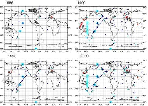
Fig. 2. Changes in the observational networks over time. The dark blue circles show the locations where flask samples are routinely taken and the large light blue squares show the locations of CMDL observatories where high frequency measurements are also available. Red circles are measurement sites that were not used because the transport model could not simulate them well. Aircraft sampling sites are shown as dark blue stars.
again in the flux estimation. The net result is that some data have effectively more weight in the inversions.
One strategy that is often employed to deal with significant gaps in data records is to use sites that have nearly continu-ous observations over the entire period for which fluxes are being estimated. Hence, if the carbon fluxes over the pe-riod 1980 to 2000 are being estimated, then only those sites that have a high percentage of actual measurements over this time span are used. As Fig. 2 shows, however, during the mid-1980’s, the observing network was very sparse. The number of sites has increased significantly over time, with the largest network expansion occurring in the early 1990’s. As we will show, even for this period large and potentially important regions remain only indirectly constrained by ob-servations. Although using a small network consisting of sites with nearly continuous data avoids multiple use of ob-servations, the results of the inversion are inevitably more dependent on prior flux estimates since less data is used to constrain the inversion.
When first conceived, the observational network was in-tended to make weekly term measurements of long-lived atmospheric species at remote locations in order to monitor the composition of the “background” atmosphere. Hence, sites were located in remote locations where predom-inantly pristine marine boundary layer air could be sampled. Over time, the realization that continental air must be sam-pled in order to adequately constrain terrestrial biospheric fluxes at continental scales has led to an increase in the num-ber of sites that sample air influenced directly by terrestrial processes. Unfortunately, these sites are also the most diffi-cult for the transport models to simulate well, and many of these sites are not currently used in global atmospheric in-versions. As models improve, it will become possible to use more of these sites.
Peylin et al. (2005). We define four networks representing the 1980’s (29 sites), 1990–1995 (48 sites), 1995–2000 (103 sites) and 2000–2002 (120 sites). A list of these sites, and time periods over which each is used is given in Table 1. The last column of Table 1 gives the model-data mismatch error chosen for each site. Sites that are not well-simulated by the transport model were excluded from each network as de-scribed in the previous section and are shown as red symbols in Fig. 2. Use of these changing networks results in abrupt adjustments in the flux estimates at the transitions between the networks, and reflects the uncertainty due to sparse and variable networks which effectively limits the ability to char-acterize any flux trends.
4 The resolution kernel
A useful diagnostic of flux estimation frameworks is the reso-lution kernel (e.g. Backus and Gilbert, 1970; Tarantola, 1987; Menke, 1989; Rodgers, 2000). This quantity indicates the degree to which the estimated parameters can be resolved in-dependently, and is equivalent to the averaging kernel matrix used in satellite retrievals. The resolution kernel may be ob-tained by assuming that the true, but unknown, values of the parameter being estimated, strue, are related to (error-free)
observations, z, by
z=Hstrue (1)
where H in this context is a matrix of the responses at each measurement site from unit pulses emitted from each source region.
The discrete Kalman filter update equation for the esti-mated source vector is (Kalman, 1960; Gelb, 1974)
s’=sp+QHT[R+HQHT]−1(z−Hsp) (2)
where Q and R are prior flux and model-data mismatch error covariance matrices, spis a vector of prior flux estimates, and
s’ is a vector of posterior flux estimates. Equations (1) and (2) may be combined as s’−sp=R
strue−sp
(3) where the resolution kernel is identified as
R=QHT[R+HQHT]−1H=KH (4) and K is the Kalman gain matrix. The resolution kernel is a square matrix with rank equal to the number of parameters estimated.
Note also that using the update equation for the covari-ance,
Q’=Q−QHT[R+HQHT]−1HQ (5) implies
Q’=(I−R)Q (6)
Individual rows ofRshow the relative extent to which each parameter may be distinguished from the other estimated pa-rameters.Rquantifies the ability to retrieve the true param-eters, with limitations due to transport errors, non-resolved local source variability and the sparseness of observations. 4.1 Limiting behavior ofRand dependence on input
parameters
It is instructive to consider the resolution kernel in terms of idealized limiting cases that show how the ability to re-solve fluxes is affected by uncertainties in prior fluxes and the model-data mismatch error. A related issue is the sparse ob-servation network which also affects resolution through pop-ulation of the response function matrix, H.
In the limit that H is a square, non-singular matrix (a singular matrix would be unphysical) and R approaches 0 (perfect transport and no observational error),Rapproaches QHT(HT)−1Q−1H−1H=I. In this case, the estimated pa-rameters are perfectly distinguishable. From Eqs. (3) and (6), it is clear that ifR=I then we obtain the true values of the estimated parameters with zero uncertainty, the ideal situa-tion. Each row of the resolution kernel gives a value of 1.0 for the element corresponding to the estimated parameter, and 0.0 elsewhere, indicating no confusion of the solution with those of other estimated parameters.
On the other hand, if RQ (Q≈0.0), then R goes to 0.0. The estimated parameters are not resolved for this case, and the estimated fluxes and their uncertainties are un-changed from prior values and uncertainties. No new infor-mation is obtained about the estimated parameters. This may also be seen from Eq. (6).
The dependence of parameter resolution on the density of observations influencesRthrough the products involving H, which is generally not square or non-singular. Source regions not well-sampled by the observational network will have cor-responding small elements in H. In the limit that H actually goes to zero,Rwill also go to zero, and the estimated pa-rameters are not resolved and the papa-rameters and uncertain-ties remain at their prior values.
Atmospheric inversion problems tend to have a mixture of parameters that are well-constrained by observations, and pa-rameters for which the estimates and uncertainties do not de-viate significantly from the prior values.Ris therefore com-posed of some rows for which the element corresponding to an estimated parameter is nearly 1.0 with small off-diagonal values, and some rows for which there are numerous peaks, and some rows for which all values are nearly zero.
Table 1. Observation Sites.
Site Code 1985 1990 1995 2000 Model-Data Mismatch Error
AIA005 X X 0.4
AIA015 X X 0.4
AIA025 X X 0.4
AIA035 X X 0.4
AIA045 X X 0.4
AIA055 X X 0.4
AIA065 X X 0.4
ALT X X X X 0.6
AMS X 0.4
ASC X X X X 0.5
ASK X X 0.5
AVI X 0.5
AZR X X X X 0.6
BAL X X 1.0
BGU X X 1.1
BHD X X X X 0.4
BME X X X 0.6
BMW X X X 0.6
BRW X X X X 0.6
BSC 1.0
CAR030 X X 0.5
CAR040 X X 0.4
CAR050 X X 0.4
CAR060 X X 0.4
CAR070 X X 0.4
CAR080 X X 0.4
CBA X X X X 0.6
CFA X X 0.5
CGO X X X X 0.4
CHR X X X X 0.4
CMN 0.7
CMO X X X 0.6
COI X X 0.6
CPT X X 0.4
CRI 0.8
CRZ X X 0.4
CSJ X X X X 0.6
DAA 0.6
EIC X 0.4
ESP X X 0.7
FRD X X 1.1
GMI X X X X 0.4
GOZ 0.6
GSN 0.8
HAA005 X 0.7
HAA015 X 0.6
HAA025 X 0.6
HAA035 X 0.6
HAA045 X 0.6
HAA055 X 0.6
HAA065 X 0.6
HAA075 X 0.6
HAT X X 0.7
HBA X X X X 0.4
Table 1. Continued.
Site Code 1985 1990 1995 2000 Model-Data Mismatch Error
HUN00 1.0
HUN010 1.1
HUN048 1.1
HUN082 1.1
HUN115 1.4
ICE X X 0.6
ITN 0.8
ITN051 0.7
ITN123 0.8
IZO X X 0.5
JBN X X 0.4
KEY X X X X 0.6
KUM X X X X 0.5
KZD 0.9
KZM 0.8
LEF 1.4
LEF011 0.9
LEF030 0.7
LEF076 0.8
LEF122 0.7
LEF244 0.7
LJO X X X 0.7
LMP X 0.6
MAA X X 0.4
MBC X X 0.6
MHD X X 0.6
MID X X X X 0.6
MLO X X X X 0.4
MNM X X 0.4
MQA X X 0.4
NWR X X X X 0.5
OPW X 0.6
ORL005 X 0.9
ORL015 X 0.6
ORL025 X 0.5
ORL035 X 0.7
PALCBC 1.1
PFA015 X 0.9
PFA025 X 0.7
PFA035 X 0.7
PFA045 X 0.7
PFA055 X 0.7
PFA065 X 0.8
PFA075 X 0.7
POCS35 X X X 0.5
POCS30 X X X 0.4
POCS25 X X X 0.5
POCS20 X X X 0.6
POCS15 X X X 0.5
POCS10 X X X 0.6
POCS05 X X X 0.6
POC00 X X X 0.7
POCN05 X X X 0.6
[image:8.595.306.546.93.688.2]Table 1. Continued.
Site Code 1985 1990 1995 2000 Model-Data Mismatch Error
POCN15 X X X 0.5
POCN20 X X X 0.4
POCN25 X X X 0.4
POCN30 X X X 0.4
POCN35 X X 0.4
POCN40 X X 0.4
POCN45 X X 0.4
PRS 0.6
PSA X X X X 0.4
RPB X X X 0.5
RTA005 X 0.4
RTA015 X 0.4
RTA025 X 0.4
RTA035 X 0.4
RTA045 X 0.4
RYO 0.7
SBL X X X X 0.8
SCH 0.6
SCSN03 X 0.5
SCSN06 X 0.5
SCSN09 X 0.4
SCSN12 X 0.5
SCSN15 X 0.5
SCSN18 X 0.5
SCSN21 X 0.7
SEY X X X X 0.4
SHM X X X X 0.8
SIS 0.7
SMO X X X X 0.4
SPO X X X X 0.4
STM X X X X 0.6
insights, however, we first provide more details about the res-olution kernel and its properties.
4.2 Relation ofRto Q
For the special case where Qprioris a diagonal matrix, the
di-agonal elements of the posterior covariance matrix are given by
qnn0 =(1−rnn)qnn (7)
whereqnn0 andqnnare diagonal elements of the posterior and
prior error covariance matrices, andrnn is the
correspond-ing diagonal element of the resolution kernel matrix. From this equation we can see that the prior parameter variance is reduced more as the resolution of the parameter increases. Similarly, it may be shown that the off-diagonal elements of the posterior error covariance are
qnm0 =rnmqmm (8)
Table 1. Continued.
Site Code 1985 1990 1995 2000 Model-Data Mismatch Error
STP X X X X 0.4
SUM X 1.1
SYO X X 0.4
TAP 0.7
TDF X X 0.4
TRM X 0.6
UTA X X 0.6
UUM X X 0.6
WES 0.8
WIS X X 0.8
WKT00 1.1
WKT030 1.1
WKT061 1.1
WKT122 1.1
WKT244 1.1
WKT457 1.1
WLG X X X 0.6
WPON30 X X 0.6
WPON25 X X 0.6
WPON20 X X 0.4
WPON15 X X 0.4
WPON10 X X 0.4
WPON05 X X 0.5
WPO00 X X 0.5
WPOS05 X X 0.5
WPOS10 X X 0.5
WPOS15 X X 0.5
WPOS20 X X 0.6
WPOS25 X X 0.6
YON X 0.7
ZEP X X 0.5
Therefore, the posterior correlations between estimated parameters for a diagonal prior error covariance matrix are related to the variance of one parameter multiplied by the corresponding cross term from the resolution kernel. The latter gives a measure of how distinguishable the estimated parameter,n, is fromm.
5 Results
Fig. 3. (Top) The estimated annual total global carbon flux and uncertainty. The yellow region shows the 1σ confidence bounds, and the red crosses show the estimated global carbon flux from the zonal average model of Tans et al. (1989) (courtesy of J. Miller and T. Conway) The green crosses show the global CO2growth
rate estimated from the observed concentrations at network sites. (Bottom) Estimated global total land and ocean fluxes. The thick red line and yellow shaded area shows the global total estimated land flux and the estimated 1σ confidence bounds, the thick dark blue line and light blue shaded area shows the global total ocean flux estimates and 1σconfidence bounds.
include the first year of the estimates since about a half year is required for the inversion to adjust from initial conditions. We also integrate our discussion of the flux estimates with the resolution kernel, since we consider the latter to be a use-ful tool in the interpretation of the flux estimates. The reso-lution kernel will be shown row by row, where the diagonal element of each row indicates how well the parameter is re-solved, and the off diagonal elements give an indication of the degree to which parameters may be distinguished from each other. We consider values greater than 0.75 to be large, and less than 0.4 to be small in the discussion below. 5.1 Carbon flux estimates at global scales
The upper panel of Fig. 3 shows the estimated annual aver-age global net carbon fluxes aggregated from 22 source re-gions. Although we have used the time-dependent network construction described in the previous section, differences
due to network configuration are small and well within the estimated errors. The 1σ confidence interval decreases sub-stantially as the network size increases over time, ranging from just under 1.0 GtC yr−1to about 0.5 GtC yr−1. The net global fluxes vary considerably, ranging from nearly zero up-take in 1987 and 1998 to upup-take of more than 3.0 GtC yr−1 during the early 1990’s. Previous studies have suggested a connection between El Ni˜no/ENSO and reductions in car-bon uptake by the biosphere and oceans (e.g. Conway et al., 1994; Feely et al., 1999, 2002; Keeling et al., 1995; Rayner and Law, 1999; R¨odenbeck et al., 2003a; Patra et al., 2005). As shown in Fig. 3, the estimated global uptake of CO2was
nearly zero during the strong El Ni˜no’s of 1987 and 1998. The early 1990’s were also a period of positive ENSO index (Wolter and Timlin, 1993, 1998); however, cooler and wetter conditions due to the major Pinatubo volcanic eruption likely caused the increased uptake during the early 1990’s, and may have also affected the response of the carbon cycle to the El Ni˜no during this period (Conway et al., 1994; Ciais et al., 1995). The flux anomalies associated with the 1997/1998 El Ni˜no shown in this study agree well with those of R¨odenbeck et al. (2003a), Bousquet et al. (2000), Gurney et al. (2008), and Rayner et al. (1999) although they are smaller than those reported by Patra et al. (2005).
Figure 3 also shows global total fluxes calculated with the zonal average model described by Tans et al. (1989) (red crosses, upper panel). This flux estimation procedure does not use prior flux estimates. The zonal average model uses only zonally averaged observations and transport to infer the carbon fluxes. The agreement between the flux estimates from this study and the zonal average technique is very good, which is expected since both calculations use the same obser-vations, and therefore must recover the same global growth rate. However, comparing the two different calculations pro-vides a useful check on the overall consistency of the flux estimates. Flux estimates can fail to match the zonal aver-age model global total fluxes if, for example, the solution is very tightly constrained to match the prior flux estimates. Also shown are the global growth rates of CO2 estimated
directly from the observed concentrations at network sites. With the exception of a few years, the agreement is quite good, even though there are errors associated with calcu-lating the global growth rate directly from observations that are mostly at the surface. A comparison to observed global growth of atmospheric CO2was also done by Rayner et al.
(2005) for their assimilation system that optimizes terres-trial biosphere model parameters. They found general agree-ment with the timing of estimated growth anomalies with differences in magnitudes that they attributed to the lack of biomass burning in their terrestrial biosphere model. Com-parisons to global growth of atmospheric flux can be a valu-able diagnostic for atmospheric inversions.
[image:10.595.66.264.60.345.2]Fig. 4. The resolution kernel for the global land and oceans in July calculated by aggregating monthly average basis functions, prior flux uncertainties, and mismatch error to global scales. Note that the resolution kernel shows how well the global land and oceans are resolved relative to each other within a particular month, as well as the degree to which the estimate for July is confused with the estimates for global ocean and land regions from previous and suc-cessive months. The “L” and “O” on the horizontal axis denote land and ocean regions for the month of interest and for adjacent time steps.
1998 El Ni˜no, the 1σ confidence intervals for the annual ter-restrial biosphere and ocean fluxes overlap. It is question-able whether there is enough spatial information such that the inversion can tell global land and ocean sources apart. Although the appropriate cross terms of the covariance ma-trix could provide insight, we show the average resolution kernel (Fig. 4), obtained by calculating the resolution ker-nel using aggregated response function, prior flux uncertainty and model-data mismatch error matrices. Figure 4 shows that the global partitioning between land and ocean fluxes is re-solvable using even early networks (implying the latter pos-sibility) where values of the diagonal element reach at least 0.7. There is little tendency for the solutions for the global oceans and biosphere to be confused either within a particu-lar month, or between adjacent months since the off-diagonal elements of the resolution kernel are very small; less than 0.2. The inversion is able to better distinguish the global total ocean and land fluxes as the network expands, espe-cially for Northern Continental regions. The ability of
at-Fig. 5. As for at-Fig. 4, except that land-sea asymmetries in prior flux covariance and model-data mismatch error have been removed by setting each matrix to the Identity matrix. Note that the resolution is dependent on the relative sizes of each a priori error, and this figure is intended to suggest the importance of a priori information in determining the resolution. Note that the black line represents the resolution kernel for the 2000 network from Fig. 4.
mospheric inversions to distinguish between global land and ocean fluxes was also noted by R¨odenbeck et al. (2003b). They obtained similar land/ocean partitioning even when dif-ferent prior fluxes were used.
It is important to recognize that the relative sizes of the global land and ocean prior flux uncertainties and the larger model-data mismatch errors for continental sites play an im-portant role in the ability to distinguish global land and ocean fluxes. This may be seen from Fig. 5, where land-sea asym-metries in these quantities are eliminated from both the prior flux covariance and the model-data mismatch errors by us-ing the same values for both ocean and land. Although the resolution of global ocean and land fluxes is also dependent on the relative sizes of the prior flux covariance and model-data mismatch error, this figure illustrates the importance of a priori information and how it contributes to the spatial dis-tribution of estimated fluxes. The a priori error estimates of ocean carbon fluxes are usually much smaller than prior ter-restrial flux error estimates, and this plays a significant role in constraining the optimization.
As for the global net flux, the 1σ confidence interval for the global annual terrestrial biosphere flux estimate de-creases from a maximum of about 1.5 GtC yr−1 to about
1.0 GtC yr−1with increasing network coverage (Fig. 3b). In
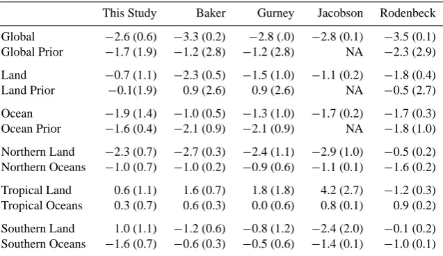
[image:11.595.48.281.64.349.2]Table 2. Comparison of 1992–1996 Average Carbon Fluxes Estimated by This Study and Those of Baker et al. (2006), Gurney et al. (2004), Jacobson et al. (2007) and R¨odenbeck et al. (2003a). The numbers in the parentheses are estimated uncertainties.
This Study Baker Gurney Jacobson Rodenbeck
Global −2.6 (0.6) −3.3 (0.2) −2.8 (.0) −2.8 (0.1) −3.5 (0.1) Global Prior −1.7 (1.9) −1.2 (2.8) −1.2 (2.8) NA −2.3 (2.9)
Land −0.7 (1.1) −2.3 (0.5) −1.5 (1.0) −1.1 (0.2) −1.8 (0.4) Land Prior −0.1(1.9) 0.9 (2.6) 0.9 (2.6) NA −0.5 (2.7)
Ocean −1.9 (1.4) −1.0 (0.5) −1.3 (1.0) −1.7 (0.2) −1.7 (0.3) Ocean Prior −1.6 (0.4) −2.1 (0.9) −2.1 (0.9) NA −1.8 (1.0)
Northern Land −2.3 (0.7) −2.7 (0.3) −2.4 (1.1) −2.9 (1.0) −0.5 (0.2) Northern Oceans −1.0 (0.7) −1.0 (0.2) −0.9 (0.6) −1.1 (0.1) −1.6 (0.2)
Tropical Land 0.6 (1.1) 1.6 (0.7) 1.8 (1.8) 4.2 (2.7) −1.2 (0.3) Tropical Oceans 0.3 (0.7) 0.6 (0.3) 0.0 (0.6) 0.8 (0.1) 0.9 (0.2)
Southern Land 1.0 (1.1) −1.2 (0.6) −0.8 (1.2) −2.4 (2.0) −0.1 (0.2) Southern Oceans −1.6 (0.7) −0.6 (0.3) −0.5 (0.6) −1.4 (0.1) −1.0 (0.1)
network are slightly larger than for the global total annual fluxes, but are still well within the estimated 1σ confidence intervals. The results shown here are consistent with those found by Gurney et al. (2008) and Patra et al. (2005) for the Transcom 3 ensemble of transport models. In their studies, they estimated fluxes for a variety of networks and found that global aggregated land and ocean fluxes are not very sensi-tive to network changes, a result that we confirm here.
The global land and ocean fluxes over the period 1994 to 2001 are in good agreement with estimates obtained using measurements of O2/N2over the period 1994–2003 obtained
by Bender et al. (2005). They find an average terrestrial up-take of 0.8–1.0±0.6 GtC yr−1and an average ocean uptake
of 1.7–2.1±0.5, while aggregated estimates for this study are 0.7±1.0 GtC yr−1and−1.9±1.2 GtC yr−1. The
inter-annual variability of the carbon fluxes estimated in this study, including the large terrestrial response to the 1998 El Ni˜no, are also comparable to the results of Bender et al. (2005), although we find less interannual variability for the ocean fluxes.
Table 2 shows a comparison of our global total, land and ocean fluxes with those published recently. The studies by Gurney et al. (2004) and Jacobson et al. (2007) use a global mass constraint derived from observations, and therefore agree with the observed global CO2 growth rate shown in
Fig. 3 averaged over 1992 to 1996 (2.8 GtC yr−1). Our
av-erage global flux is slightly less than the observed value and this is consistent with the influence of the global prior flux, which is considerably smaller than the observed value due to a neutral biosphere. The results of Baker et al. (2006) and R¨odenbeck et al. (2003a) show a much larger than observed global uptake of carbon. Baker et al. (2006) note that the global growth obtained from the observations they used were 0.3 GtC yr−1smaller than that used by Gurney et al. (2004),
and this along with slightly larger fossil fuel emissions ac-counts for the difference in the global fluxes. It is interesting that even for the global total flux, there can be significant differences between the flux estimates, and we note that all studies shown used the same fossil fuel inputs, albeit with small differences that my arise through interpolation.
The average global ocean fluxes shown in Table 2 may be grouped into two categories, with Baker et al. (2006) and Gurney et al. (2004) showing much less uptake by oceans than the other three studies. Not surprisingly, these studies show more uptake by the global terrestrial biosphere. Note that the joint inversion of Jacobson et al. (2007) and the study by R¨odenbeck et al. (2003a) use ocean carbon measurements to constrain ocean fluxes, making the agreement between these calculations of ocean uptake very good.
5.2 Zonal average carbon flux estimates
Table 3. Definition of Land and Ocean Zones (Numbers correspond to those used in the Figures).
Zone TransCom 3 Region
High N. Land (1) Boreal N America (1) Boreal Eurasia (7)
Temperate N. Land (2) Temp. N America (2) Temp. Asia (8) Europe (11) Tropical Land (3) Amazonia (3) N. Africa (5) SE Asia (9) Temperate S. Land (4) Temp. S America (4) S Africa (6) Australia (10) High N. Oce. (5) Northern Oce. (16)
Temperate N. Oce. (6) N Pacific (12) N Atlantic (17)
Tropical Oce. (7) W/E Eq. Pacific (13,14) Eq. Atlantic (18) Eq. Ind. Oce. (21) Temperate S. Oce. (8) S Pacific (15) S Atlantic (19) Temp.Ind. Oce. (22) High Southern Oce. (9) Southern Oce. (20)
they have corresponding peaks of less than 0.2. For the re-cent networks, the resolution of these regions is significantly improved. For the less well-sampled Tropical and Southern Hemisphere zones much of the inversion’s ability to separate land and ocean fluxes comes from land-ocean asymmetries in prior flux uncertainty (as for the global land-sea flux par-titioning).
The aggregated zonal land flux estimates and uncertainties are shown in Fig. 7. Effects of changes in network config-uration are evident at this spatial scale, particularly for the Temperate Northern Hemisphere Land where the number of observing sites has increased significantly with time. In con-trast, the jumps are not as large for the Temperate South-ern Hemisphere and SouthSouth-ern Ocean zones, where the num-ber of observing sites has increased less. Note the decreases in the 1σ confidence intervals for the Northern Hemisphere Land zones, and the small decrease in the tropical land zone. As the size of the network increases and the estimated error decreases, the estimates for ocean and land regions become more distinguishable.
As the number of sampling sites constraining the Temper-ate Land regions increases, the estimTemper-ated carbon uptake in-creases significantly. This may imply that the earlier, sparser networks produce biases towards underestimation of uptake, but it is also possible that there are model biases relating to vertical mixing influence the inversion increasingly as more sites directly sample continental air. The increased uptake in the Northern temperate land zone occurs at the expense of uptake over the less well-constrained tropical land regions.
Figure 7 suggests that the large response to the 1998 El Ni˜no event occurred in tropical land regions where carbon was emitted to the atmosphere at a rate of about 2.0 GtC yr−1.
This agrees well with the flux estimates of R¨odenbeck et al. (2003a), Peylin et al. (2005), Rayner et al. (2008), Patra et al. (2005) and van der Werf et al. (2004), and with analyses that suggest warm, dry conditions over the tropics resulted in in-creased respiration and biomass burning (Zeng, 1999). It is interesting that for the 1987 El Ni˜no no comparably large sig-nal is found for the tropical land zone, however, there were fewer observations in the tropics during the 1980’s, while
more recently, shipboard observations and other sites have been added at low latitudes.
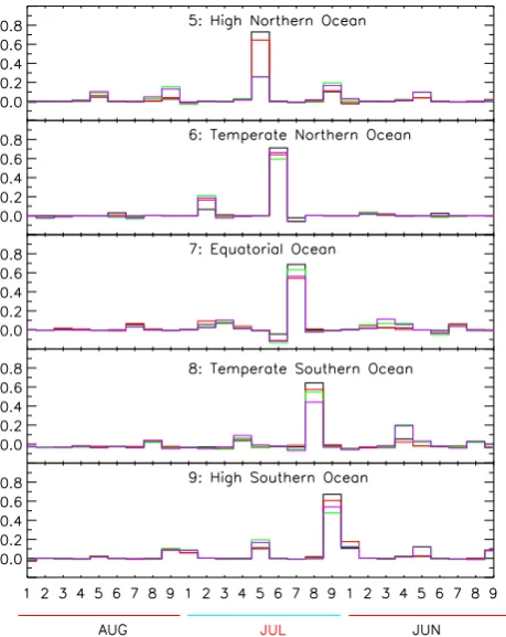
The resolution kernel for the zonal ocean regions (Fig. 8) shows that the Northern Hemisphere ocean zones are rela-tively well-resolved (diagonal elements greater than about 0.75) for the most recent networks, however, the diagonal elements for the Southern Hemisphere Ocean regions are closer to 0.6. It is interesting that the inability to distinguish between the solution for a particular ocean region and an ad-jacent land region seems to be smaller than that between land and neighboring ocean regions. This is likely a result of the historical preference for locating network sites in the marine boundary layer in order to sample background atmospheric CO2abundances.
Figures 6 and 8 suggest that for the 2000 network, and to a lesser extent, the 1995 network, the Equatorial and Southern Temperate Ocean and Land zones are fairly well-resolved. It is important to keep in mind, however, that the zonal es-timates reflect the fluxes near to the (mostly surface) mea-surements. The zonal average flux for tropical land regions for example, does not include direct measurements of Trop-ical South America, and hence the response of the zonal av-erage Tropical land fluxes to climate variability does not di-rectly inform on the response of the ecosystems of Amazonia to such perturbations. Zonal (and global) aggregations are prone to errors and biases arising from the sparse underlying sampling distribution.
[image:13.595.117.478.88.210.2]Fig. 6. The resolution kernel for approximately zonal land regions in July, calculated by aggregating monthly average basis functions, prior flux uncertainties, and mismatch error for the TransCom 3 re-gions. Note that the resolution kernel shows how well the zonal land regions are resolved within the month of July, as well as the degree to which the solutions for July are confused with solutions for zonal oceans and land from previous and successive months. The num-bers on the horizontal axis indicate the zonal regions as follows: 1 – High Northern Land, 2 – Temperate Northern Land, 3 – Tropical Land, 4 – Temperate Southern Land, 5 – High Northern Ocean, 6 – Temperate Northern Oceans, 7 – Tropical Oceans, 8 – Temperate Southern Oceans, 9 – High Southern Ocean. Note also that the res-olution kernel for the different networks as described in the text are shown: 2000 (black), 1995 (red), 1990 (green) and 1985 (purple).
It has recently been suggested by Stephens et al. (2007), using aircraft observations independent of flux inversions, that many of the models used to estimated carbon fluxes have transport biases that result in overestimated uptake by the ter-restrial Northern Hemisphere and a corresponding overesti-mate of emissions by the terrestrial Tropics. They point out that the Transcom 3 Level 2 models that most closely match the annual observed CO2profiles obtain flux estimates for the
[image:14.595.313.542.61.332.2]Northern Extra-Tropics and Tropical fluxes of−1.5 (±0.6) and 0.1 (±0.8) GtC yr−1. Figure 3 of Stephens et al. (2007) suggests that larger Northern uptake and Tropical emission are also (non-unique) solutions that agree with the observed vertical profile. In light of this, our average estimated up-take of−2.3 (±0.7) GtC yr−1for the Northern lands and 0.6
Fig. 7. Aggregated estimates of quasi-zonal land (red) and ocean (blue) fluxes. The shaded areas indicate the estimated 1σ con-fidence bounds for the estimated land fluxes (yellow) and ocean fluxes (light blue). The jumps in the solution are the results of using time-varying networks as described in the text.
(±1.1) GtC yr−1for the Tropical lands are not necessarily
in-consistent with the results of Stephens et al. (2007), however compensation by Southern land and ocean regions must also be considered.
The flux estimates for the Northern Oceans are similar for all of the studies in Table 2 except for R¨odenbeck et al. (2003a) which shows more uptake, perhaps to compensate for less Northern land uptake. The range of the tropical ocean fluxes is quite large, with emissions ranging from 0 to 0.9 GtC yr−1. All flux estimates, except for those of Gur-ney et al. (2004) agree to within the estimated errors with the estimate of Jacobson et al. (2007) which are constrained by ocean observations. On the other hand, only the estimates from this study agree with those of Jacobson et al. (2007) for the Southern oceans.
5.3 Continental and ocean basin-scale carbon flux estimates
Fig. 8. The resolution kernel for approximately zonal ocean regions in July, calculated by aggregating monthly average basis functions, prior flux uncertainties, and mismatch error for the TransCom 3 re-gions. The numbers on the horizontal axis relate to the zonal regions as follows: 1 – High North Land, 2 – Temperate North Land, 3 – Tropical Land, 4 – Temperate South Land, 5 – High North Ocean, 6 – Temperate North Oceans, 7 – Tropical Oceans, 8 – Temperate South Oceans, 9 – High South Ocean. Note also that the resolution kernel for the different networks as described in the text are shown: 2000 (black), 1995 (red), 1990 (green) and 1985 (purple).
The resolution kernel for the terrestrial TransCom 3 re-gions is shown in Fig. 9. Carbon fluxes estimated for Bo-real and Temperate North America are readily distinguish-able from the adjacent Northern Ocean and North Atlantic regions, although the diagonal elements have increased with network expansions from 0.6 or less to values of 0.8. For many regions, the resolution has substantially increased as the network has expanded. This is especially true for Aus-tralia, Europe and Southeast Asia where the diagonal values were initially 0.2 or less and have reached 0.75 or more for recent networks. On the other hand, source regions in South America, Africa and Boreal Eurasia are less well-resolved. In particular, South America is not resolved at all having di-agonal values less than 0.2, while North Africa is resolved to some extent for the 1995 and 2000 networks (diagonal val-ues increasing from about 0.2 to 0.5), due to the addition of sites in Algeria and the Middle East. Southern Africa is gen-erally not distinguishable from the Equatorial and South
At-Fig. 9a. The resolution kernel for TransCom 3 terrestrial regions 1–6 in July. The numbers on the horizontal axis correspond to the individual TransCom regions as follows: 1 – Boreal North America, 2 – Temperate North America, 3 – Amazonia, 4 – Temperate South America, 5 – North Africa, 6 – South Africa. Note also that the res-olution kernel for the different networks as described in the text are shown: 2000 (black), 1995 (red), 1990 (green) and 1985 (purple).
lantic ocean regions since the diagonal values and the peak corresponding to the South Atlantic are both about 0.4 and of comparable size. The ability to resolve Boreal Eurasian fluxes has increased slowly (going from 0.3 to 0.6), but the solution for this region is not entirely distinguishable from the adjacent Northern Ocean and North Pacific and Atlantic regions since there are corresponding peaks for these regions of about 0.2.
[image:15.595.50.280.63.352.2]Fig. 9b. The resolution kernel for TransCom 3 terrestrial regions 7–11 in July. The numbers on the horizontal axis correspond to the individual TransCom regions as follows: 7 – Boreal Eurasia, 8 – Temperate Eurasia, 9 – Southeast Asia, 10 – Australia, 11 – Europe. Note also that the resolution kernel for the different networks as described in the text are shown: 2000 (black), 1995 (red), 1990 (green) and 1985 (purple).
zonal average fluxes for the Tropical Land regions are a weighted combination of the observational constraints for Southeast Asia, and the prior flux estimates for other Tropical regions. It is therefore difficult to draw conclusions about re-sponses of individual tropical land regions to large perturba-tions, such as the 1998 El Ni˜no using even current networks. Figure 10 shows the resulting annual average flux and un-certainty estimates for the 11 TransCom terrestrial regions. At High Northern latitudes, the abrupt changes in estimated fluxes due to changes in the network are evident, especially for Europe where the coverage has increased significantly in recent years. The estimated flux uncertainties decrease for all three High Northern latitude regions as the network expands in time. Note that although the estimated flux for Boreal North America remains relatively constant, ranging between about 0.0 and 0.5 GtC yr−1, there is a large rebalancing of up-take from Europe to Boreal Eurasia. The upup-take of carbon for Europe decreases from greater than about 2 GtC yr−1to an emission averaging about 0.5 GtC yr−1from the late 1980’s to the late 1990’s, while the estimates for fluxes over Bo-real Eurasia change from nearly a 1 GtC yr−1source to about a 1 GtC yr−1 sink. It is somewhat surprising that Europe
Fig. 10. Estimates of annual average terrestrial fluxes for the 11 TransCom 3 terrestrial source regions. The shaded yellow areas in-dicate the estimated 1σconfidence bounds for the estimated fluxes. The blue curve show the flux estimates calculated using the 2000 network for the entire period.
[image:16.595.309.544.63.377.2]observations are used (e.g. time averaging or missing data criteria applied). However, the conclusion is that changing networks are likely to be a source of “noise” and uncertainty that must be considered when long time series of flux esti-mates are computed for the evaluation of trends. Further-more, the unrealistic change in estimated fluxes underscores the care that must be taken when using difficult to model con-tinental sites. It is possible to control fluctuations of flux es-timates by tuning the model-data mismatch errors to dampen variations. The result would be greater influence of prior flux estimates and/or reduced spatial resolution of flux estimates. The best solution, as always, is better transport models and increased observational coverage.
Carbon flux estimates for Temperate North America have remained relatively constant over time at about−1 GtC yr−1, however, the uptake of carbon for the 2000 network was greatly reduced by over half. Carbon uptake appears to be increasing towards 1 GtC yr−1 again during 2001 and
2002. Flux estimates calculated using the 2000 network (blue curve) shows smaller uptake over the entire period. These figures illustrate a fundamental difficulty in dealing with a sparse network that increases in resolution unevenly in space and slowly in time; it is difficult to attribute changes in estimated fluxes solely to biophysical processes unless sen-sitivity to network changes is considered as well.
As shown above, of the tropical land regions, only South-east Asia is well-resolved, although the 1σconfidence inter-val for North Africa is significantly reduced after the addi-tion of a site in Northern Africa and one in the Middle East (namely, ASK and WIS). Southeast Asia appears to be a sig-nificant sink of carbon except for the period during the late 1990’s when shipboard observations in the South China Sea were included in the estimation (the shipboard observations were discontinued and not included in the 2000 network). Although the quality of these shipboard data does not seem to be in question (Conway, personal communication), either their inclusion or exclusion appears to introduce a large bias in the calculation. It has been suggested by Arellano et al. (2004) and Petron et al. (2002) that the anthropogenic carbon monoxide (CO) emissions from Southeast Asia have been significantly underestimated, and this may be an explanation for why the biosphere in this region seems to become a large source when the South China Sea observations are included. It is interesting that all tropical land regions show small decreases in uptake for 1998. The variations are small com-pared to changes due to network composition, and they are small compared to the 1σconfidence intervals as well. Since Tropical Africa, Tropical South America, and sometimes, Southeast Asia cannot be distinguished from each other (and from adjacent ocean regions), it is likely that the 1998 El Ni˜no response is distributed in a somewhat even fashion over the tropical land regions.
[image:17.595.311.539.58.383.2]Of the Temperate Southern Land regions, only Australia is well-resolved after about 1995. The flux estimates sug-gest that Australia is a small source of atmospheric carbon.
Fig. 11a. The resolution kernel for TransCom 3 ocean regions 12– 17 in July. The numbers on the horizontal axis correspond to the individual TransCom regions as follows: 12 – North Pacific, 13 – Western Tropical Pacific, 14 – Eastern Tropical Pacific, 15 – South Pacific, 16 – Northern Ocean, 17 – North Atlantic. Note also that the resolution kernel for the different networks as described in the text are shown: 2000 (black), 1995 (red), 1990 (green) and 1985 (purple).
Estimated fluxes for Southern Africa and Temperate South America appear to roughly balance each other after 1995.
Fig. 11b. The resolution kernel for TransCom 3 ocean regions 18– 22 in July. The numbers on the horizontal axis correspond to the individual TransCom regions as follows: 18 – Equatorial Atlantic, 19 – South Atlantic, 20 – Southern Ocean, 21 – Tropical Indian Ocean, 22 – Temperate Indian Ocean. Note also that the resolution kernel for the different networks as described in the text are shown: 2000 (black), 1995 (red), 1990 (green) and 1985 (purple).
At high latitudes, the Southern Ocean is fairly well-resolved (with diagonal values greater than 0.75 for all net-works) while the solution for the Northern Ocean has a di-agonal element between 0.7 and 0.75 for all networks, with small (0.2) peaks indicating that the ability to distinguish the Northern Ocean from Boreal North America and Eurasia is somewhat limited. Note that there is a noticeable amount of “leakage” of signal between Boreal North America, Eurasia and the Northern Ocean as evidenced by peaks in the reso-lution kernels among these regions. On the other hand, the solutions for Temperate North America and Eurasia, and the Northern Atlantic and Pacific Oceans are more distinguish-able.
Estimated fluxes and uncertainties for the TransCom ocean regions are shown in Fig. 12. The results are consistent with the idea that high latitude oceans are sinks of atmospheric carbon dioxide, while the tropical oceans are sources. Note that most ocean regions are sensitive to changes in network configuration. Regions with sparse observational coverage over the entire period are less sensitive to network changes over time. Examples are the Equatorial and South Atlantic and the Equatorial and Temperate Indian Oceans.
Fig. 12. Estimates of annual average ocean fluxes for the 11 TransCom 3 ocean source regions. The shaded yellow areas indicate the estimated 1σ confidence bounds for the estimated fluxes.The blue curve show the flux estimates calculated using the 2000 net-work for the entire period.
Significant estimated uptake occurs over the Northern Ocean, North Atlantic and the Southern Ocean. Tans et al. (1990) and, more recently, Gurney et al. (2002) have pointed out that all of the models used in the TransCom 3 model intercomparison suggested that the Takahashi et al. (1999) ocean flux data used as a prior for the inversions are too high for the Southern Ocean by a factor of two, possibly due to a seasonal bias in the deltapCO2measurements. Our results
are consistent with their findings, showing uptake of about 0.5 GtC yr−1for the Southern Ocean.
The largest estimated oceanic source of atmospheric car-bon is found over the Eastern Equatorial Pacific and appears to be about 0.5 GtC yr−1±0.5 GtC yr−1. It is noteworthy
[image:18.595.309.545.64.369.2]Fig. 13. Average seasonal cycles of estimated flux and uncertainty for the well-resolved TransCom 3 terrestrial source regions (plus Boreal Eurasia, which is not well-resolved).The black lines and shaded yellow areas indicate the estimated fluxes and 1σconfidence bounds using the 2000 network. The red line is the prior flux es-timate taken from the CASA model and the blue line shows flux estimates calculated using the 1990 network.
The average seasonal cycles of estimated and prior terres-trial fluxes using the 2000 network are shown in Fig. 13. For Boreal North America, the estimates suggest a more shallow summertime uptake than the prior flux estimates, with a more gradual onset of summertime uptake. For Europe, the flux estimates suggest more emission to the atmosphere during the winter and slightly more uptake than the prior flux esti-mate. The flux estimates for Boreal Eurasia revise the prior flux significantly, increasing the uptake during the growing season by almost a factor of two. Note that the prior flux es-timate is balanced annually and may undereses-timate the true uptake. Although the results of Gurney et al. (2004) also show a larger estimated summertime uptake for Boreal Eura-sia than the prior flux estimate, the results shown in Figure 13 differ from the results of Gurney et al. (2004) in that the win-ter respiration fluxes are little changed from the prior, while the uptake during the growing season is significantly larger than the prior estimates. Figures 9 and 11 suggest that Boreal Eurasia is the least distinguishable region at high Northern latitudes, and the large increases in uptake are likely the re-sult of the high prior flux uncertainty for this region. It is also interesting that the peak carbon uptake estimated by Gurney et al. (2004) is distributed more evenly between Europe and Boreal Eurasia, whereas our results show less European up-take and more for Boreal Eurasia. This difference is due to
our use of more observation sites, since the partitioning of flux between these two regions is very dependent on network composition. Model transport biases may also play a role in the adjustment towards less summer uptake for Europe.
In the Temperate Northern Hemisphere, the flux estimates suggest that the summer uptake occurs earlier than it does for the prior fluxes by about a month for the most recent network. For the more sparse 1990 network, the timing of the summer uptake occurs later than for the prior. In the case of Tem-perate Eurasia, the timing of the summertime uptake is also shifted earlier, especially for the more recent network. Less carbon emission during the Northern Hemisphere winter is estimated for both Temperate North America and Temperate Eurasia (for the 2000 network), and the latter is a carbon sink throughout most of the year.
The only tropical terrestrial source region that is well-resolved is Southeast Asia, where the inverse flux estimates for the 2000 network suggest considerable seasonality while the prior flux estimate is rather flat. A peak in emissions oc-curs during the Northern Hemisphere summer, and the sea-sonality of the flux estimates is likely related to the Asian summer monsoon cycle.
Temperate South American flux estimates are not signifi-cantly changed from the prior flux estimate due to the lack of observations to constrain this region. On the other hand, the seasonality suggested by the prior flux estimates for South-ern Africa are discarded by the inversion, which produces a rather flat seasonal cycle centered around zero instead. Note that the resolution kernel for this region suggest some confu-sion with the estimated flux for the adjacent South Atlantic. The flux estimates for Australia (which is well-resolved for the 2000 network and not resolved for the 1990 network) are also interesting, since they imply a net positive flux of carbon dioxide to the atmosphere, with a peak in emissions occur-ring duoccur-ring Austral Autumn for the recent network. The prior and 1990 network flux estimates, on the other hand, show small uptake of carbon over the Austral winter that peaks in early Austral spring.