SPECTRAL DIMENSIONALITY REDUCTION BASED ON
INTERGRATED BISPECTRUM PHASE FOR
HYPERSPECTRAL IMAGE ANALYSIS
Khairul Muzzammil Saipullah
aand Deok-Hwan Kim
ba
Faculty of Electronic and Computer Engineering,
Universiti Teknikal Malaysia Melaka, Malysia
b
Dept. of Electronic Engineering, Inha University, South Korea
ABSTRACT
In this paper, we propose a method to reduce spectral dimension based on the phase of integrated bispectrum. Because of the excellent and robust information extracted from the bispectrum, the proposed method can achieve high spectral classification accuracy even with low dimensional feature. The classification accuracy of bispectrum with one dimensional feature is 98.8%, whereas those of principle component analysis (PCA) and independent component analysis (ICA) are 41.2% and 63.9%, respectively. The unsupervised segmentation accuracy of bispectrum is also 20% and 40% greater than those of PCA and ICA, respectively.
Keywords: dimensionality reduction, bispectrum, hyperspectral image segmentation
1. INTRODUCTION
With the development of the hyperspectral sensor, researchers in the remote sensing field are now able to extract ample spectral information to identify and discriminate between spectral similarity of materials. The hyperspectral image (HSI) covers large number of bands which results in more accurate and detailed information of each material than those of other remotely sensed data, as in the multispectral image. A typical HSI covers up to several hundreds of bands. Although HSI provides more information, it has some downfalls. The irrationally large dimension of HSI requires extremely high computational complexity. The large number of dimensions also causes degradation in classification accuracy .1 It is because HSI contains a huge amount of spectral redundancy .2 Therefore, the reduction of spectral dimensionality is necessary in order to perform the classification or target detection.
The most widely used algorithm for dimensionality reduction in the remote sensing field is the principal component analysis (PCA) .3PCA computes orthogonal projections that maximize the amount of data variance, and yields a dataset in a new uncorrelated coordinate system. An improvement of PCA is the independent component analysis (ICA)4which uses higher order statistics. Some other methods utilize multiscale approaches such as derivative spectroscopy5 and the wavelet transform 6 to extract relevant features from hyperspectral signals. In derivative spectroscopy, smoothing operator and derivative operator are used to detect “hills” and “valleys” in the spectral curves while in wavelet transform, the means of systematically analyzing hyperspectral curves via windows of varying width are applied.
Although all the dimensionality reduction methods are able to reduce the number of spectral band, the effectiveness of the dimensionality reduction feature is low. Especially for spectral that is reduced from hundreds dimension to one dimension (1D), the discriminating power of the resulting 1D feature are small. Therefore, the usage of this 1D reduced feature will result in low classification accuracy. From the evaluation in literature ,2 the number of effective dimensional reduced feature of PCA for spectral classification is larger than twenty dimensions.
Further author information: (Send correspondence to Deok-Hwan Kim)
K. M. Saipullah: E-mail: muzzammil@utem.edu.my, Telephone: +33 (0)1 98 76 54 32 Deok-Hwan Kim: E-mail: deokhwan@inha.ac.kr, Telephone: +82 32 860 7424
In this paper, we propose a method to reduce spectral dimension based on the phase of integrated bispectrum. Based on the area size of the integrated bispectrum, the resulting phase can be split into a number of features. The resulting feature vectors are then used to represent the spectral of each pixel in the hyperspectral image. Because of the excellent information extracted by the bispectrum, the resulting feature has high discriminating power even with only single dimension data. The phase of the integrated bispectrum feature is tested on spectral classification and HSI segmentation.
The remainder of this paper is organized as follows: in Section 2, related work is presented; in Section 3, detailed algorithm of the proposed dimensionality reduction based on the integrated bispectrum phase is presented; experimental evaluations are described in Section 4 and finally conclusions and future works are given in Section 5.
2. RELATED WORKS
2.1 Principle Component Analysis
Milton et al. 3 used PCA to reduce the dimensionality of spectra. The spectra can be converted to the relevant dimensionality by a linear transformation with the significant eigenvectors computed from PCA. When the eigenvectors are convolved with the spectra, it transforms the spectra into fewer data points. The eigenvectors are determined by computing the covariance matrix of the mean of the spectral data matrix as opposed to the covariance about the origin as follows:
[Cjk] = n i=1XijXik− n i=1Xijni=1Xik N N−1 (1)
where [Cjk] is the covariance matrix of the mean, X is a single band measurement, N is the number of spectra in the matrix,j,kare indices over spectral bands, andi is an index over the number of spectra. The covariance matrix is then diagonalized by finding a matrix [Q] such that
[Q]−1[C][Q] = [λ][I] (2)
where [I] is the identity matrix. The columns of matrix [Q] are the eigenvectors and the column matrix [λ] is the corresponding eigenvalues. Then matrix [λ] is sorted in descending order. The resulting PCA feature is the element of matrix [Q] corresponding to the sorted eigenvalues indices. The sorted matrix [Q] is also called the principle component of the spectra data. The principle component is sorted from the significant eigenvectors to the less significant eigenvectors. These eigenvectors are then used as the feature vectors of the spectra.
2.2 Independent Component Analysis
The goal of principle component analysis is to minimize the reprojection error from compressed data. On the other hand, the goal of independent component analysis is to minimize the statistical dependence between the basis vectors. Mathematically, this calculation can be written as follows:
WXT =U (3)
where the ICA finds the linear transformationWthat minimizes the statistical dependence between the rows of Ugiven by data matrixX. The basis vectors in ICA are neither orthogonal nor ranked in order. There are a lot of algorithms in finding the transformationW. In this paper, we will use the algorithm proposed by T. Kolenda .7 This ICA algorithm is an enhanced version of Molgedey and Schuster algorithm4with a fast computation of the model. LetXτ ={Xj,t+τ}be the time shifted data matrix. The lag parameterτis automatically determined by exploiting the difference between the autocorrelations of the data matrix X. Then using the singular value decomposition (SVD), the principle component subspace is calculated by decomposing
Figure 1. The segmentation of bispectrum. The quotient matrix can now be written as:
ˆ Q= 1
2D(V T
τV+VTVτ)D−1= ΦΛΦ−1 (5)
The Φ contains the rectangular ICA basis projection onto the PCA subspace andU holds the projection from the PCA subspace. The estimated mixing matrix and the source signals are given by
A=UΦ (6)
S= Φ−1DVT (7)
Φ can be selected according the significant principle components. By only selecting certain number of signif-icant principle components after the SVD, the dimension of the input data can be reduced. The final estimated source signalsSare used as the feature vectors of the input data.
3. THE PROPOSED DIMENSIONALITY REDUCTION
3.1 Higher Order Spectra
Higher order spectra (HOS) were introduced as spectral representations of cumulants or moments of ergodic processes .8 It is useful in the identification of nonlinear and non-Gaussian random processes, as well as deter-ministic signals. The use of higher order spectra for feature extraction is based on its properties such as they retain both amplitude and phase information of the signal, they are robust to signal modifications, and they have zero expected value for Gaussian noise .9 Because of the extra information, robustness and high immunity to Gaussian noise, we implement the higher order spectra to reduce the dimensionality of the HSI.
3.1.1 Bispectrum
Polyspectra are defined as the Fourier transform of moment and cumulate statistics. Bispectrum is the polyspec-tra with third order and can be calculated as follows :9
B(f1, f2) =X(f1)X(f2)X∗(f1+f2) (8) where |f1| ≤1,|f2| ≤1,|f1+f2| ≤ 1,X∗(f) is the complex conjugate ofX(f) andX(f) can be calculated as follows: X(f) = 1 N N−1 n=0 x(n)e−j2πnfN (9)
wherex(n) is the discrete-time transient signal withN samples.
Bispectrum can be segmented into twelve sectors as shown in Fig. 1 and the first sector is an infinite wedge bounded byf1=f2. Due to the symmetry property of bispectrum for real-valued signal, the sector 1 in Fig. 1 is commonly used for analysis and refereed as non-redundant sector. In order to only obtain the sector 1 of the bispectrum, we can limit the condition for formula (8) with 0≤f1≤f2≤f1+f2≤1.
3.1.2 Integrated Bispectrum
The integrated bispectrum is computed by integrating radially along slices in the sector 1 of the bi-frequency plane .9, 10 This approach was motivated by the need to obtain certain invariant properties that are meaningful in pattern recognition. The bispectrum can be integrated using the following formula:
I(a) =
N
2−1/1+a
f1=1
B(f1, af1) (10)
whereN is the number of sample and 0< a≤1. The bispectrum is interpolated using the following formula:
B(f1, af1) =pB(f1,af1) + (1−p)B(f1,af1) (11) wherexis the largest integer inx,xis the smallest integer inx,B(x, y) is the bispectrum from formula (8) andpis calculated as follows:
p=af1− af1 (12)
3.2 The Feature Extraction
The result of the integrated bispectrum I is a complex number which contains the magnitude and the phase. Because of the translation, dc-level, amplification, and scale invariant of the phase ,9 it is selected to be the feature of the signal. The phase of the integrated bispectrum is calculated as follows:
P(a) = tan−1Im{I(a)}
Re{I(a)} (13)
The number of dimensions of the final feature vector is depending on the number of parameter aused in in formula (13). The final feature vector set of the integrated bispectrum phase is as follows:
Vk =
Pxk:x∈Z; 0< x≤k (14)
This means that V is the set of integrated bispectrum phase of xk such that xis an integer in the range from 0 to k where k is the desired dimension of the feature vector. For example, for a three dimensional feature,
V3=P13, P23, P33.
4. EXPERIMENTAL STUDIES
This section discusses the experimental studies regarding the performance of the dimensionality reduction meth-ods. The methods are evaluated in terms of the spectral classification accuracy and HSI segmentation accuracy.
4.1 Experiment Setup
We carefully extract six classes of spectral from two HSI. The list and the number of spectra are listed in Table 1. Two HSIs used in this experiment are the Seoul HSI (Upper left L/L: 37.661257N/126.785989E , Lower right L/L: 37.510587N/126.922847E) and Seosan HSI (Upper left L/L: 36.742125N/126.521865E, Lower right L/L: 37.510587N/126.922847E). The resolution of each HSIs are 559x403 and 439x367 pixels with a scale of 30m per pixel. RGB band images of these HSIs are shown in Fig. 2. These HSIs are captured using Hyperion sensors with a total of 229 bands. After removing the noise, the remaining bands are 145 bands with the wavelength in range from nm to 406.46nm to 2496.39nm.
Due to the various range of feature dimensions, the nearest neighbor classifier with Euclidean distance is chose to classify the spectra. A cross-validation scheme is applied in order to reduce the dependency on the training set. Each class of the spectral is equally divided into four groups and for each pair of groups, one group is used as testing set and the other is used as training set. Because we divided the spectral into four groups, by replacing the testing and training set with each of the group, there are twelve classifications will be conducted. The average of these twelve classification accuracy is recorded as the overall classification accuracy. The classification and segmentation performance of the Bispectrum is compared to those of PCA and ICA, respectively.
Table 1. The class and the number of spectra used in the classification experiment. Class Number of spectra
Water 1000 Buildup 1000 Barren 1000 Grass 1000 Coniferous 2000 Agricultural 2000
(a) Seoul HSI (b) Seosan HSI
Figure 2. The RGB band images of Seoul and Seosan HSIs.
4.2 Classification Experiment
The spectral classification is conducted according to the measures discussed in the section 4.1. For each method, the classification is repeated 100 times using different feature dimension size in the range from 1 to 100 dimensions. The overall classification accuracies for bispectrum, PCA and ICA are shown in Fig. 3. At the smaller dimensional feature size, the classification accuracies of ICA are higher than those of PCA. However, at the larger dimensional feature size, the classification accuracies of PCA outdo the accuracies of ICA. We can see that the classification accuracies of bispectrum are consistent and high even for small dimensional feature size. This shows that bispectrum is able to optimizing the dimensionality reduction effectively compared to those of PCA and ICA, respectively. The best overall classification accuracy for each method is shown in Table 2. In this table, we also included the classification accuracy using the original spectral feature. The highest classification accuracy is achieved by the bispectrum with only four dimensional feature. The classification accuracies of PCA, ICA and
Table 2. The best classification accuracy for bispectrum, PCA, ICA and spectral features. Method Bispectrum PCA ICA Spectral
Dimension 4 100 99 145 Water 99.20 98.46 97.13 97.40 Buildup 97.60 97.34 95.55 97.20 Barren 96.86 95.35 94.82 95.80 Grass 100.00 99.15 99.35 98.30 Coniferous 100.00 99.65 99.73 99.78 Agricultural 99.93 99.18 99.20 98.28 Average 98.93 98.19 97.63 97.79
(a) Image in RGB bands (b) The ground truth image
Figure 4. The HSI used in the segmentation experiment.
spectral are still lower than those of bispectrum even with hundreds dimensional features.
4.3 Segmentation Experiment
For the segmentation experiment, we conducted an unsupervised segmentation of a HSI using the K-mean clustering algorithm with Euclidean distance .11 The RGB band images of the HSI and its ground truth images are shown in Fig. 4. The HSI contains 288 bands including the noise and is divided into four regions which are the water, buildup, grass & trees and agricultural regions. 4-mean clustering is applied to cluster the pixels into those four regions. We compared the performance of the bispectrum, PCA and ICA using the one dimensional feature.
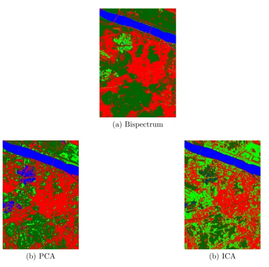
The segmentation result of the HSI is shown in Fig. 5 and the segmentation accuracies for the bispectrum, PCA and ICA is shown in Table 3. We can clearly see that the segmentation result of the bispectrum is similar to the ground truth image. This is because of the high discriminating characteristic of the one dimensional bispectrum feature. Although the ICA performs well than PCA in the classification experiment using small dimension feature size, the segmentation result of ICA is the worst. The difficulty in discriminating the grass & trees class and the agricultural causes ICA to mix up the pixels of those two classes.
Table 3. The HSI segmentation accuracies. Method Bispectrum PCA ICA Accuracy (%) 90.19 70.05 51.65
(a) Bispectrum
(b) PCA (b) ICA
Figure 5. The segmentation result using Bispectrum, PCA and ICA with 1D feature.
5. CONCLUSIONS AND FUTURE WORKS
In this paper, we proposed a dimensionality reduction method based on the integrated bispectrum phase. Most of the dimensionality reduction methods are unable to perform effectively with lower dimensional feature. However the bispectrum is able to overcome this problem due to its high discriminating feature.
The bispectrum feature is based on pixel-wise operation and only relies on spectral properties of the data alone. For HSI land-cover classification application, the information related to the spatial arrangement of the pixels is important. The future work of bispectrum is to incorporate the spatial arrangement in the feature extraction.
5.1 Acknowledgments
This research was supported in part by the MKE(The Ministry of Knowledge Economy), Korea, under the CITRC(Convergence Information Technology Research Center) support program(NIPA-2011-C6150-1102-0001) supervised by the NIPA(National IT Industry Promotion Agency) and in part by Basic Science Research Program through the National Research Foundation of Korea(NRF) funded by the Ministry of Education, Science and Technology (2011-0004114) and in part by the Defense Acquisition Program Administration and Agency for Defense Development, Korea, through the Image Information Research Center at Korea Advanced Institute of Science and Technology under the contract UD100006CD and in part by Universiti Teknikal Malaysia Melaka.
REFERENCES
[1] Landgrebe, D., “Hyperspectral image data analysis,”Signal Processing Magazine, IEEE 19, 17 –28 (Jan. 2002).
[2] Renard, N., Bourennane, S., and Blanc-Talon, J., “Denoising and dimensionality reduction using multilinear tools for hyperspectral images,”Geoscience and Rem. Sens. Letters, IEEE5(2), 138 –142 (2008).
[3] Smith, M. O., Johnson, P. E., and Adams, J. B., “Quantitative determination of mineral types and abun-dances from reflectance spectra using principal components analysis,” in [Lunar and Planetary Science Conf. Procs.], 15, 797–804 (Feb. 1985).
[4] Molgedey, L. and Schuster, H., “Separation of independent signals using time-delayed correlations,”Physical Review Letters72(23), 3634–3637 (1994).
[5] Tsai, F. and Philpot, W., “Derivative analysis of hyperspectral data,”Remote Sensing of Environment66(1), 41 – 51 (1998).
[6] Bruce, L., Koger, C., and Li, J., “Dimensionality reduction of hyperspectral data using discrete wavelet transform feature extraction,” Geoscience and Remote Sensing, IEEE Transactions on 40, 2331 – 2338 (Oct. 2002).
[7] Kolenda, T., Hansen, L., and Larsen, J., “Signal detection using ica: Application to chat room topic spotting,”In proc. ICA’20015, 3197–3200 (2001).
[8] Brillinger, D. R., “An introduction to polyspectra,”The Annals of Mathematical Statistics36(5), pp. 1351– 1374 (1965).
[9] Chandran, V. and Elgar, S., “Pattern recognition using invariants defined from higher order spectra- one dimensional inputs,”Signal Processing, IEEE Transactions on41, 205 (Jan. 1993).
[10] Chandran, V., Carswell, B., Boashash, B., and Elgar, S., “Pattern recognition using invariants defined from higher order spectra: 2-d image inputs,”Image Processing, IEEE Transactions on6, 703 –712 (May 1997). [11] MacQueen, J. B., “Some methods for classification and analysis of multivariate observations,” in [Proc. of the 5th Berkeley Symp. on Math. Stat. and Prob.], Cam, L. M. L. and Neyman, J., eds.,1, 281–297 (1967).