Vehicle longitudinal motion modeling for nonlinear control

Vehicle longitudinal motion modeling for nonlinear

control

Khalid El Majdoub, Fouad Giri, Hamid Ouadi, Luc Dugard, Fatima Zara

Chaoui

To cite this version:

Khalid El Majdoub, Fouad Giri, Hamid Ouadi, Luc Dugard, Fatima Zara Chaoui. Vehicle longitudinal motion modeling for nonlinear control. Control Engineering Practice, Elsevier, 2012, 20 (1), pp.69 - 81. <10.1016/j.conengprac.2011.09.005>. <hal-00638489>

HAL Id: hal-00638489

https://hal.archives-ouvertes.fr/hal-00638489

Submitted on 7 Nov 2011

HAL is a multi-disciplinary open access

archive for the deposit and dissemination of sci-entific research documents, whether they are

pub-lished or not. The documents may come from

teaching and research institutions in France or abroad, or from public or private research centers.

L’archive ouverte pluridisciplinaire HAL, est destin´ee au d´epˆot et `a la diffusion de documents scientifiques de niveau recherche, publi´es ou non, ´emanant des ´etablissements d’enseignement et de recherche fran¸cais ou ´etrangers, des laboratoires publics ou priv´es.

Vehicle Longitudinal Motion Modeling for nonlinear control

a,* _{GREYC Lab, UMR CNRS, University of Caen Basse-Normandie, Caen, France}

b

GIPSA Lab, UMR CNRS, INPG, Grenoble, France

c _{ENSET, Universite´ de Rabat-Agdal, Rabat, Marocco}

Abstract— The problem of modeling and controlling vehicle longitudinal motion is addressed for front wheel propelled vehicles. The chassis dynamics are modeled using relevant fundamental laws taking into account aerodynamic effects and road slop variation. The longitudinal slip, resulting from tire deformation, is captured through Kiencke‟s model. A highly nonlinear model is thus obtained and based upon in vehicle longitudinal motion simulation. A simpler, but nevertheless accurate, version of that model proves to be useful in vehicle longitudinal control. For security and comfort purpose, the vehicle speed must be tightly regulated, both in acceleration and deceleration modes, despite unpredictable changes in aerodynamics efforts and road slop. To this end, a nonlinear controller is developed using the Lyapunov design technique and formally shown to meet its objectives i.e. perfect chassis and wheel speed regulation.

Keywords – vehicle longitudinal control, longitudinal slip, tire Kiencke‟s model, speed control, Lyapunov stability.

1.INTRODUCTION

Vehicle longitudinal motion control aims at ensuring passenger safety and comfort. It is an important aspect in dynamic collaborative driving i.e. when multiple vehicles should coordinate to share road efficiently while maintaining safety. In this respect, several works have been devoted to what is commonly referred to adaptive cruise control that consists in maintaining a specified headway between vehicles (Ioannou and Chien, 1993; Moon et al., 2009). Different control techniques have been used in these works including linear and adaptive control (You et al., 2009), genetic fuzzy control (Poursamad and Montazeri, 2008), sliding mode control (Liang et al., 2003; Nouveliere and Mammar, 2007), and scheduling gain control involving PIDs (Ren et al., 2008). However, most previous works on longitudinal control were based on simple models neglecting important nonlinear aspects of the vehicle such as rolling resistance, aerodynamics effects and road load. In some studies, the controller performances were not formally analyzed (Ren et al., 2008). In (Yamakawa et al., 2007), longitudinal vehicle control has been studied focusing on torque management for independent wheel drive. It is worth noticing that in all previous studies on longitudinal vehicle control, the control design has been based on simple models not accounting for tire-road interaction.

In the present study, the problem of longitudinal vehicle control is revisited, for front wheel propelled vehicles, focusing on speed regulation. The aim is to design a controller that is able to tightly regulate the chassis and wheel velocities, in both acceleration and deceleration driving modes, despite changing and uncertain driving conditions. This problem has not been dealt with previously. A further originality of the present paper is that the control design relies upon a more complete model that accounts for most vehicle nonlinear dynamics including tire-road interaction. That is, the study includes two major contributions. First, a suitable control model is developed for the vehicle longitudinal behavior. In this respect, recall that a convenient model is one that is sufficiently accurate but remains simple enough to be utilizable in control design. To meet the accuracy requirement, the model must account not only for aerodynamic phenomena but also, and especially, for tire-road friction. Modeling the tire/road contact is a quite complex issue involving multiple aspects relevant to tire characteristics (e.g. structure, pressure) and to environmental factors (e.g. road load, temperature). Several tire models have been proposed in the literature e.g. Guo‟s model (Guo and Ren, 2000), Pacejka‟s model (Pacejka and Besselink , 1997), Dugoff‟s model (Dugoff and Segel, 1970), Gim‟s model (Gim and Nikravesh, 1990), Kiencke‟s model (Kiencke and Nielsen, 2004). In the present work, Kiencke‟s model is retained because it proves to be a good compromise between accuracy and simplicity. The overall vehicle modeling is carried out according to the bicycle model principle. In addition to tire equations, the model includes chassis dynamics equations (obtained from fundamental dynamics and aerodynamics laws) and incorporates relevant practical prior knowledge e.g. the tire longitudinal slip is physically limited. The overall vehicle model turns out to be a combination of two nonlinear state-space representations describing, respectively, the acceleration and deceleration longitudinal driving modes. Its high complexity makes it hardly utilizable for control design but, due to its high accuracy, it proves to be quite suitable for simulator building. This model development is one major achievement of the present study. The second contribution is the design of a nonlinear controller that ensures global stabilization and longitudinal speed regulation during acceleration/deceleration driving modes. This is carried out using the Lyapunov design technique (Khalil, 2002), based on a simpler (but still accurate) version of the above simulation-oriented model. It is formally proved that the developed controller actually achieves the stability and regulation objectives it was designed to. Furthermore, it is observed through numerical simulations that the controller is quite robust with respect to uncertainties on environmental characteristics.

The paper is organized as follows: Section II is devoted to modeling the acceleration/deceleration vehicle longitudinal behavior; the obtained model is used in Section III to design a controller and to analyze the resulting closed-loop system; the controller performances are illustrated in Section IV by numerical simulations. A conclusion and reference list end the paper.

2.MODELLING OF CHASSIS LONGITUDINAL MOTION

Except for aerodynamic forces, all external efforts acting on a vehicle are generated at the wheel-road contact. The understanding and modeling of the forces and torques developed at wheel-road contact is essential for studying properly the vehicle dynamics. These are discussed in the forthcoming subsections. In this respect, recall that the vehicle motion is composed of two types of displacements: translations along the

x

,

y

,

z

2.1. Kiencke’s Tire Modeling

The tire is a main component of the wheel-road contact as it ensures three important functions (Kiencke and Nielsen, 2004): (i) bearing the vertical load and absorbing road deformations; (ii) producing longitudinal acceleration efforts and contributing to vehicle braking; (iii) producing the required transversal efforts that help the vehicle turning.

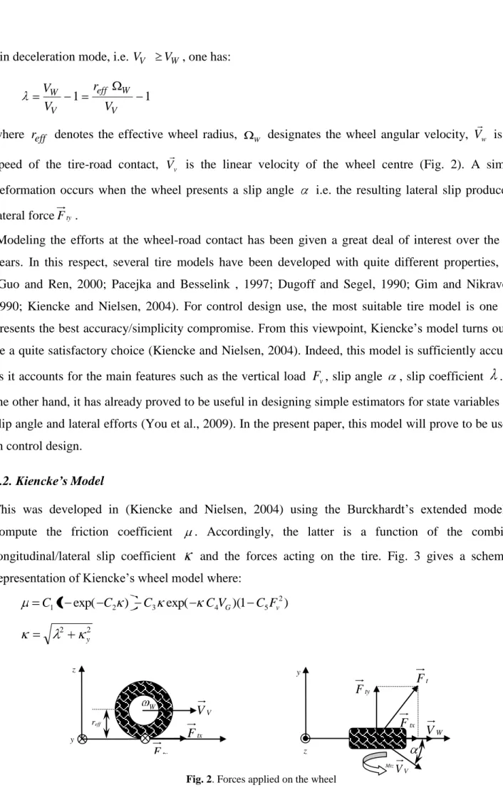
The efforts generated at the wheel-road contact include longitudinal (acceleration/deceleration) forces, lateral guiding forces and self alignment torque. The effect of these efforts on the vehicle behaviour is determined by the tire-road adhesion. For small load variations, the longitudinal coefficient of friction is characterized by the following ratio:

v tx F F

(1) where F_tx denotes the longitudinal effort and F_v the vertical load. The ratio is called longitudinal adhesion or friction coefficient. The value of this coefficient depends on the tire slip resulting from the deformation of the tire in contact with the road (Kiencke and Nielsen, 2004). The longitudinal slip is characterized by the coefficient defined as follows:

. in acceleration mode, i.e. V_V V_W, one has:

W eff V W V r V V V 1 1 (2) Longitudinal motion Vertical motion x y z ψ φ Roll _Pitch

Fig. 1. Degrees of freedom of a vehicle

Transversal motion

. in deceleration mode, i.e. V_V V_W , one has: 1 1 V W eff V W V r V V (3)

where r_eff denotes the effective wheel radius, _W designates the wheel angular velocity, Vw



is the speed of the tire-road contact, V_v is the linear velocity of the wheel centre (Fig. 2). A similar deformation occurs when the wheel presents a slip angle i.e. the resulting lateral slip produces a lateral forceFty.

Modeling the efforts at the wheel-road contact has been given a great deal of interest over the last years. In this respect, several tire models have been developed with quite different properties, e.g. (Guo and Ren, 2000; Pacejka and Besselink , 1997; Dugoff and Segel, 1990; Gim and Nikravesh, 1990; Kiencke and Nielsen, 2004). For control design use, the most suitable tire model is one that presents the best accuracy/simplicity compromise. From this viewpoint, Kiencke‟s model turns out to be a quite satisfactory choice (Kiencke and Nielsen, 2004). Indeed, this model is sufficiently accurate as it accounts for the main features such as the vertical load F_v, slip angle , slip coefficient . On the other hand, it has already proved to be useful in designing simple estimators for state variables like slip angle and lateral efforts (You et al., 2009). In the present paper, this model will prove to be useful in control design.

2.2. Kiencke’s Model

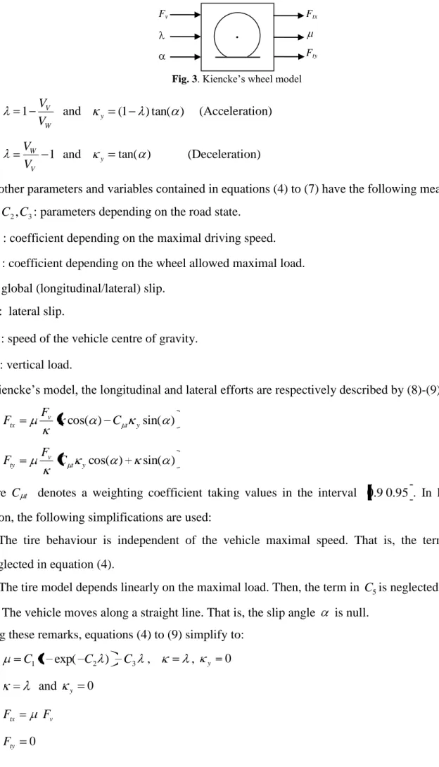
This was developed in (Kiencke and Nielsen, 2004) using the Burckhardt‟s extended model to compute the friction coefficient . Accordingly, the latter is a function of the combined longitudinal/lateral slip coefficient and the forces acting on the tire. Fig. 3 gives a schematic representation of Kiencke‟s wheel model where:

) 1 )( exp( ) exp( 1 _{2 3 4 5} 2 1 C C CVG C Fv C (4) 2 2 y (5) y z t F ty F tx F W V V V y z V V tx F ty F W

Fig. 2. Forces applied on the wheel reff

W V

V V

1 and _y (1 )tan( ) (Acceleration) (6)

1

V W

V V

and y tan( ) (Deceleration) (7)

The other parameters and variables contained in equations (4) to (7) have the following meanings: 3

2 1,C ,C

C : parameters depending on the road state. 4

C : coefficient depending on the maximal driving speed. 5

C : coefficient depending on the wheel allowed maximal load. : global (longitudinal/lateral) slip.

y: lateral slip. G

V : speed of the vehicle centre of gravity.

V

F : vertical load.

In Kiencke‟s model, the longitudinal and lateral efforts are respectively described by (8)-(9): ) sin( ) cos( _{t y} v tx C F F (8) ) sin( ) cos( y t v ty C F F (9)

where C t denotes a weighting coefficient taking values in the interval 0.90.95 . In longitudinal

motion, the following simplifications are used:

(i) The tire behaviour is independent of the vehicle maximal speed. That is, the term in C₄ is

neglected in equation (4).

(ii) The tire model depends linearly on the maximal load. Then, the term in C₅is neglected in (4).

(iii) The vehicle moves along a straight line. That is, the slip angle is null. Using these remarks, equations (4) to (9) simplify to:

3 2 1 1 exp( C ) C C , , y 0 (10) and y 0 (11) v tx F F (12) 0 ty F (13)

Fig. 3. Kiencke‟s wheel model

Fv Ftx

2.3. Rolling Resistance and Aerodynamic Resistance

It is obvious that tire deformation causes mechanical losses. Radial deformations are caused by the vertical load. Fig. 4 shows that the vertical force distribution (along the deformation area) is not uniform. The resulting force moves from the central point I to a point located at a distance drr,max (Fig

4). This is called vertical load maximal trail and is defined as follows:

eff rr

rr r

d ,max (14)

When the wheel starts moving, a torque is generated provided that d_rr,max 0. To bring back the

vertical load strength to the central point I , a compensating torque M_rr must be applied (by the driving motor) on the wheel. This is called rolling resistance torque and is given by:

eff rr v rr v rr F d F r M ,max (15) 2.4. Aerodynamic Resistance

Aerodynamic resistance has naturally an impact on energy consumption onboard. Fluid mechanics laws are resorted to explain air flow around a moving vehicle. Accordingly, vehicle forms are continuously reinvented to improve aerodynamic performances (Power and Nicastri, 2000). Aerodynamic efforts come in direct interaction with the vehicle, producing various forces (drag, lift and lateral) which in turn generate torques (yaw, roll and pitch). The aerodynamic drag force is significant when the vehicle moves at grand speed. The aerodynamic lift effort increases the rolling resistance (because the surface of tire-road contact grows up) improving tire steerability. On the other hand, the aerodynamic lift force decreases the vehicle adhesion which reduces its stability and security (Milliken and Milliken, 1995). In presence of front-wind, the aerodynamic resistance is represented by two forces: the aerodynamic drag force Faex and the aerodynamic lift force Faez. These are defined as

follows: 2 2 ) ( 2 1 ) ( 2 1 a V z aez a V x aex V V S C F V V S C F (16) v F drr reff W I

with:

: air density depending on atmosphere pressure and ambient temperature. Cx : aerodynamic drag coefficient.

Cz : aerodynamic lift coefficient. S : frontal projection area vehicle. VV: vehicle speed.

Va : wind speed (positive in presence of front-wind, negative in presence of rear-wind).

2.5. Modeling of a Wheel Submitted to Driving Couple

Fig. 5 shows a one-wheel vehicle with mass M_v. The wheel is driven by a couple M_m. Let J denotes the inertia resulting from the wheel, the transmission shaft and the driving motor. Invoking the dynamic fundamental principle, one gets the following equation:

rr eff t W m Fr M dt d J M (18)

where equation (15) has been used to account for the rolling resistance. Using the relation VW reff W,

one gets: rr eff v eff t m eff w M Fr Fr J r V (19)

Equation (19) together with (1), (2), (3) and (10) describe the one-wheel vehicle behavior. This is further illustrated by the schematic representation of Fig. 6.

2.6. Model of Two-Wheel Vehicle with One Driving Wheel

Longitudinal and transversal behaviors can be assumed to be decoupled when the steering angle is small. Then, we make use of the vehicle symmetry to perform a projection (of all forces) on the longitudinal axis reducing thus the four-wheel model into a (two-wheel). Fig. 7 illustrates the forces involved in a bicycle model. The involved notations are described in Table I. Now, the focus will be made on the bicycle model considering that only one wheel is submitted to a motor torque M_m. For vehicle stability purpose, the front wheel is driving. The distribution of the vehicle load over the tires is computed applying the two dynamic fundamental laws. Doing so, one gets the following equations:

v v aex v tf M g F M V F ( sin )  (20) 0 ) cos ( _{v aez} vr vf F M g F F (21) 0 ) (F F h l F l F_{vf f vr r tf tr} (22)

Fig. 5. One-wheel vehicle model Fig. 6. Schematic representation of a one-wheel vehicle submitted to a driving couple

g M F g M F g V g M F v aex v aez v v vf (1 )cos ( sin ) (1 )  (23) g M F g M F g V g M F v aex v aez v v vr cos ( sin )  (24) where r f l l h and r f f l l l

. From equation (20) it is easily seen that the vehicle speed

undergoes the following equation: ) sin ( 1 aex v tf v v F M g F M V (25)

TABLE I. NOTATIONS OF VEHICLE LONGITUDINAL MODEL.

lf : Distance between CoG and the front wheel base (m) lr : Distance between CoG and the rear wheel base (m) l : Distance between the bases of the two wheels (m)

h : Height of the gravity centre (m)

Faex : Aerodynamic drag force (N)

Faez : Aerodynamic carrying force (N)

g : Gravity acceleration (m.s-2)

Mv : Vehicle mass (kg)

Ftf, Ftr : Front and rear wheel drive force (N) Fvf, Fvr : Load on the front and rear wheel (N)

θ : Road slop (rad)

h lf lr aex F tf F aez F tr F vf F vr F CoG g M Mvg

Fig. 7. The forces acting on a bicycle typevehicle

Fv Vv VW Ft Mm Body of mass Mv W t F v F

2.7. State-Space Representation of Vehicle Longitudinal Behavior

The equations obtained so far are now combined together to build-up a state-space representation of the vehicle longitudinal acceleration/deceleration behavior. The vehicle longitudinal dynamics are characterized by two state variables, i.e. vehicle (chassis) speed V_v and front-wheel speed V_w. As the

slip coefficient depends on the current driving mode (acceleration or deceleration), the vehicle is characterized by two state-space representations. Each representation describes the vehicle in the corresponding operation mode.

2.7.1. State-Space Representation in Deceleration Mode Vw Vv

Combining (3), (10), (11), (13) and (15)-(18), one obtains the following state-space representation: 2 7 6 5 1 4 3 2 1 exp( ) ( v a) v w v w v w m w V V V V V V V V M V ₈ ( )2 ₉exp( ) ₁₀( )2exp( ) v w a v v w a v v w V V V V V V V V V V (26a) 2 15 14 13 1 4 3 2 2 12 11 ( ) exp( ) ( v a) v w v w v w a v v V V V V V V V V V V V ( ) 17exp( ) 18( )2exp( ) 2 16 v w a v v w a v v w V V V V V V V V V V (26b) where the various parameters are defined in Table II. A more compact representation of (26a-b) is obtained introducing the notations:u M_m, x₁ V_w, x₂ V_v and:

2 2 7 2 1 6 5 1 2 1 4 2 1 3 2 2 1 1( , ) exp( ) (x Va) x x x x x x x x f ( ) exp( ) ( ) exp( ) 2 1 2 2 10 2 1 9 2 2 2 1 8 x x V x x x V x x x a a (27a) 2 2 15 2 1 14 13 1 2 1 4 2 1 3 2 2 2 12 11 2 1 2( , ) ( a) exp( ) (x Va) x x x x x x V x x x f ( ) exp( ) ( ) exp( ) 2 1 2 2 18 2 1 17 2 2 2 1 16 x x V x x x V x x x a a (27b)

With the above notations, the state-space representation (26a-b) is given the following usual compact form: ) , ( ) , ( 2 1 2 2 2 1 1 1 1 x x f x x x f u x   (28)

TABLE II.DEFINITION OF THE MODEL PARAMETERS

Vehicle parameters in deceleration Vehicle parameters in acceleration : 2 C ' : C₂ 1 : J reff 1 ' : J r_eff 2 : 1 k_v(C₁ C₃) ' : ₂ 1 k_v(C₁ C₃) 3 : kv C3 ' : ₃ kv C3 4 : kv C1exp(C2) '4 : kv C1exp( C2) 5 : J r C C k g Mv rr v eff 2 3 1 )) ( ( cos ) 1 ( '5 : J r C C k g M_{v rr v} eff 2 3 1 )) ( ( cos ) 1 ( 6 : J r C k g M_{v v} eff 2 3 cos ) 1 ( ' : 6 J r C k g M_{v v} eff 2 3 cos ) 1 ( 7 _: J r C C k SC_{z rr v} eff 2 3 1 )) ( ( ) 1 ( 2 1 7 ' : J r C C k SC_{z rr v} eff 2 3 1 )) ( ( ) 1 ( 2 1 8 : J r C k SC ) 1 ( 2 1 eff2 3 v z 8 ' : J r C k SC_{z v} eff 2 3 ) 1 ( 2 1 9 : J r C C k g M_{v v} eff 2 2 1exp( ) cos ) 1 ( '9 : J r C C k g M_{v v} eff 2 2 1exp( ) cos ) 1 ( 10 _: J r C C k SCz v eff 2 2 1exp( ) ) 1 ( 2 1 10 ' : J r ) C exp( C k SC ) 1 ( 2 1 eff2 2 1 v z 11 gsin( ) '11 : gsin( ) 12 _: x v SC M 2 1 ' 12 : x v SC M 2 1 13 : (1 )gcos kv(C1 C3) '13 : (1 )gcos kv(C1 C3) 14 : (1 )gcos kvC3 '14 : (1 )gcos kvC3 15 _{: (1 ) SC k (C C )} M 2 1 3 1 v z v 15 ' : (1 ) SC k (C C ) M 2 1 3 1 v z v 16 : 3 ) 1 ( 2 1 C k SC M_v z v 16 ' _: 3 ) 1 ( 2 1 C k SC M_v z v

17 : (1 )gcos kvC1exp(C2) '17 : (1 )gcos kvC1exp( C2) 18 : ) exp( ) 1 ( 2 1 2 1 C C k SC M_v z v 18 ' : _{(1 ) exp( )} 2 1 2 1 C C k SC Mv z v

2.7.2. State-Space Representation in Acceleration Mode V_v V_w

Using (2), (10), (11), (13) and (15)-(18), one gets the following state-space representation: 2 7 ' 6 ' 5 ' 1 ' 4 ' 3 ' 2 ' 1 ' _{exp( ) ( )} a v w v w v w v m w V V V V V V V V M V '8 ( )2 '9exp( ' ) '10( )2exp( ' ) w v a v w v a v w v V V V V V V V V V V (29a)

2 15 ' 14 ' 13 ' 1 ' 4 ' 3 ' 2 ' 2 12 ' 11 ' ) ( ) exp( ) ( _{v a} w v w v w v a v v V V V V V V V V V V V '16 ( )2 '17exp( ' ) '18( )2exp( ' ) w v a v w v a v w v V V V V V V V V V V (29b) where the various parameters are defined in Table II. Let us introduce the notations:

2 2 1 2 8 ' 2 2 7 ' 1 2 6 ' 5 ' 1 1 2 ' 4 ' 1 2 3 ' 2 ' 2 1 ' 1( , ) exp( ) ( a) (x Va) x x V x x x x x x x x x f exp( ) ( ) exp( ) 1 2 ' 2 2 10 ' 1 2 ' 9 ' x x V x x x a (30a) 2 2 15 ' 1 2 14 ' 13 ' 1 1 2 ' 4 ' 1 2 3 ' 2 ' 2 2 12 ' 11 ' 2 1 ' 2( , ) ( a) exp( ) (x Va) x x x x x x V x x x f ( ) exp( ) ( ) exp( ) 1 2 ' 2 2 18 ' 1 2 ' 17 ' 2 2 1 2 16 ' x x V x x x V x x x a a (30b)

where u,x1andx2 are as in (27a-b). With these notations, the state-space representation (30a-b) is given the following more compact form:

) , ( ) , ( 2 1 ' 2 2 2 1 ' 1 ' 1 1 x x f x x x f u x   (31)

2.8 Control- and Simulation-Oriented Models for Two-Wheel Vehicle With Single Driving Wheel

2.8.1 Control-Oriented Models

2.8.1.1 Control-Oriented Model Accounting For Tire Dynamics

Combining the mode-dependent state space representations (28) and (31), one gets a single model representing the vehicle in all operation modes i.e.

) , ( ) , ( ) , ( 2 1 2 2 2 1 1 2 1 * 1 1 x x g x x x g u x x x   (32) with: ) , ( ) , ( 1 ) , ( ) , ( ) , ( _{1 2 1 2 1 1 2 1 2 1}' _{1 2} 1 x x x x f x x x x f x x g (33a) ) , ( ) , ( 1 ) , ( ) , ( ) , ( _{1 2 1 2 2 1 2 1 2 2}' _{1 2} 2 x x x x f x x x x f x x g (33b) ' 1 2 1 1 2 1 2 1 * 1(x,x ) (x,x ) 1 (x,x ) (33c) 2 ) ( 1 ) , ( 1 2 2 1 x x sign x x (33d)

In addition to vehicle aerodynamics, this model does account for tire-road contact effect. Furthermore, it will prove to be useful in control design (Section III).

2.8.1.2 Control-Oriented Model Ignoring Tire Dynamics

To better appreciate the benefit of accounting of tire-road contact, a comparison will be performed in Section IV between the controller obtained from (32)-(33) and the one obtained from a simplified model neglecting tire-road contact. Specifically, the simplified model is obtained letting 0 (tire sliding negligence) which immediately implies that V_v V_w (i.e. x1 x2). Ignoring also the rolling

resistance _rr, one gets invoking the dynamic fundamentals principles for translation and rotation:

eff tf m eff w M F r J r V (34) ) sin ( 1 aex v tf v v F M g F M V (35)

where F_aexis defined by (16). It is readily seen from (34)-(35) that the vehicle speed undergoes the following equation: 2 2 2 2 ( ) 2 1 sin _{x v a} v v eff v eff m v eff eff v SC V V M g M r J M r M M r J r V (36)

where the different parameters are defined in Table V. Introduce the following notations:

v eff eff M r J r 2 (37a) 2 2 2 2 2 ( ) 2 1 sin ) ( x a v v eff v eff V x SC M g M r J M r x f (37b)

Then, equation (36) can be given by the following more compact form where u M_m and x₂ V_v:

) ( 2

2 u f x

x (38)

The first-order equation (38) is a simplified version of the second-order model (32)-(33). As already mentioned, both models will be based upon in control design and the obtained controllers will be compared later in Section IV.

2.8.2 Simulation Model

Obvious physical considerations show that in real-life longitudinal motions, the vehicle and wheel speeds are always quite close to each other. On the other hand, there is no guarantee that the model (32)-(33) ensures always that x₁ x₂. In the next lines, the model will be slightly modified so that

2 1 x

x becomes a structural property of it. Doing so, one also will discard any risk of singularity in '

1 2 ' 4 ' 1 2 3 ' 2 ' 2 1 ' 2 1 4 2 1 3 2 2 1 exp ) , ( exp ) , ( x x x x x x x x x x x x (39)

Indeed, it is readily seen that the functions and ' are continuous and:

0 exp ) , ( 0 exp ) , ( ' 4 ' 3 ' 2 ' 2 1 ' 4 3 2 2 1 x x x x if x1 x2

The continuity of and ' then guarantees the existence of _h 0 and 0 l 1, such that:

0 ) , ( inf 0 ) , ( inf 2 1 ' 1 1 2 1 1 1 2 1 2 1 x x x x h l x x x x (40)

As a matter of fact, the size of _h and _l depends on the parameters ' '

, ,

, _{i i} (i 2,3,4). The above result, shows that equations (32)-(33) are representative of the vehicle longitudinal behavior as long as the state vector (x₁,x₂) stays in the following validity domain:

h l v x x IR x x D ( , ) :1 1 2 1 2 2 1 (41)

A more realistic vehicle longitudinal model is one that structurally enforces the state variables (x₁,x₂)

to stay always in the above domain. To this end, introduce the new variable

2 1

x x

x and its

time-derivative ₂ 2 1 2 1 x x x x x

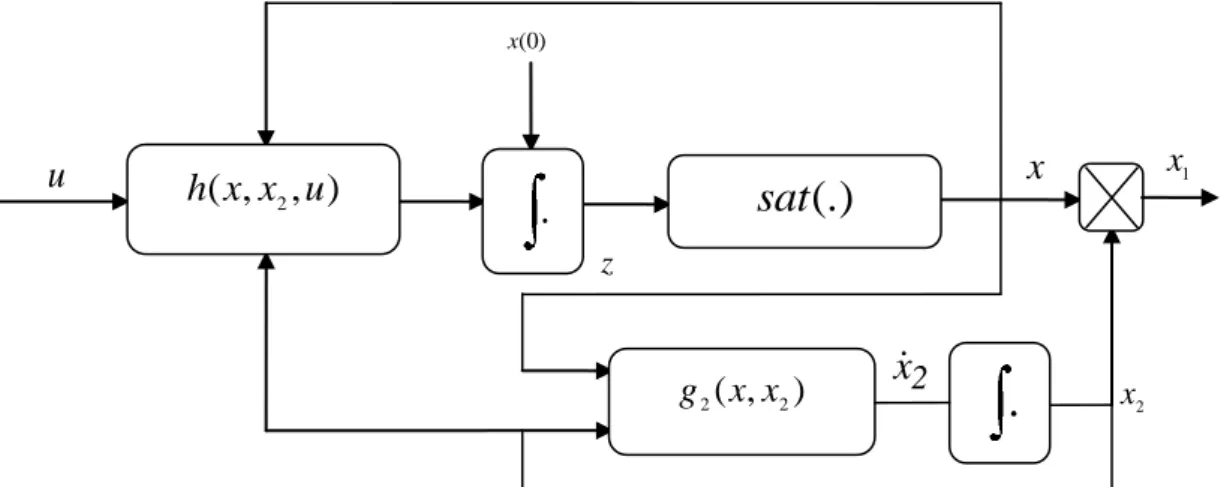
x   . Then, equation (32) can be rewritten in term of the couple (x,x₂) as follows: ) , ( ) , , ( 2 2 2 2 x x g x u x x h x   (42) with: ) , ( ) , ( 1 ) , , ( ₁* _{1 2 2 2} 2 2 u g x x xg x x x u x x h (43)

It is readily seen from (42) that: ) 0 ( ) , , ( ) ( 0h x x2 u d x t x t (44)

Then, the prior knowledge (41) is accounted for taking the saturated version of (44) i.e.:

)) ( ( ) (t sat z t x (45) with

) 0 ( ) , , ( ) ( 0h x x2 u d x t z t def (46) where sat(.) denotes the saturation function defined by:

h h h l l l z if z if z z if z sat 1 1 1 1 1 1 ) ( (47)

It is readily seen from (46) that the auxiliary variable z(t) undergoes the differential equation: ) , , ( ) (t h x x₂ u z and z(0) x(0) (48)

Then, it follows from (45) that, see Fig. 8. ) , , ( ) (z h x x2 u r x (49) where ) ( ) ( sat z dz d z r (50)

It is easily checked using (47) that r(.) is the unit rectangular function defined by:

h h l l z if z if z if z r 1 0 1 1 1 1 0 ) ( (51)

Putting the second equation in (42) together with (48)-(49), one gets the new model:

) , ( ) , , ( ) ( ) , , ( ) ( 2 2 2 2 2 x x g x u x x h r x u x x h t z    with z(0) x(0) and x1 xx2 (52)

As it accounts for the prior knowledge (47), the new model (52) turns out to be more accurate than the models (32)-(33) and (38). However, model (52) is too complex to be used for control design, due e.g. to the nonsmooth nature of the function r(z) defined by (51). Therefore, that model can (and presently will) only be used to build up simulators of the vehicle longitudinal motion. Model (32)-(33) is a quite satisfactory compromise between model (38) (simpler but less accurate) and model (52) (more accurate but more complex).

Example 1.To illustrate previous and forthcoming results, the example of a Citroën-2CV car, with the characteristics of Table VI, will be considered throughout in the rest of the paper. Using Table II and Table VI, one gets the numerical values of the parameters in the functions and ' defined by (39), see Table III.

It is readily seen, by simple checking, that conditions (40a) are fulfilled. Furthermore, it is seen from Fig. 9a that (x1,x2) 0 if 0.93 1

2 1 x x

Fig. 8. Synoptic scheme of the simulation vehicle model (52)

Figs. 9.a. (x1,x2)vsx1/x2 Fig. 9.b. '(x1,x2)vsx2/x1

TABLE III.VALUES OF THE PARAMETERS IN (34) FOR THE CITROËN-2CV CAR

Deceleration Acceleration : -23.99 ' _{: 23.99} 2 : 1.36002 ' 2 : 1.15202 3 : -0.104 ' 3 : 0.104 4 : -6714265556.98732 ' 4 : -9.76223532472411 10 -12 whenever 0 1 1 2 x x i.e. 2 1 1 x x

. In the light of these observations, it is seen that the validity

domain is 0.93 . 2 1 x x That is, 0.07 1

l and h₁ . On the other hand, the tire cannot assume

(in acceleration as well as in deceleration mode) a sliding larger than _max 10% i.e. _max.

Then, one gets from (2) and (3) that 0.9 1.11 2 1 x x which gives 0.1 2 l and h2 0.11. Letting min , 0.07 2 1 l l

l and h min h1, h2 0.11, one gets that 0.93 1.11

2 1 x x . The ) , , (x x2 u h

.

sat

(.)

x



_.

resulting bounding on the sliding turn out to be _{l h} with _{l l} 0.07 and 1 . 0 1 h h h

3. VEHICLE LONGITUDINAL REGULATORS DESIGN 3.1. Reference Trajectory Generation

We seek a speed controller for the vehicle moving in longitudinal acceleration/deceleration modes. The regulator design is based on the vehicle model (32) and the control objective is to enforce the vehicle chassis and wheel speeds, x₁ V_w and x₂ V_v, to track their reference trajectories, denoted Vw*

and Vv*, respectively. The latter are required to be time-differentiable. This requirement that can

always be complied with by pre-filtering given (non-differentiable) speed setpoints:

d w r w d v r v V s T V V s T V 1 1 1 1 * * (53a)

with V_w*(0) V_v*(0) 0, where the filter time constant T_r is freely chosen by the user and V_wd, V_vd are

positive speed setpoints. The above references cannot both be freely chosen because they are linked by (32). As a matter of fact, the desired reference of vehicle speed V_vd is first chosen by the user. Then, the wheel reference Vwd is let to be of the form:

d v d

w V

V (1 *) (53b)

where * is a constant (representing the sliding) that is uniquely obtained from (32) letting there

d v

V

x₂ , x₁ (1 *)V_vd and setting x₂ 0. Doing so, one gets g₂ (1 *)V_vd,V_vd 0, due to (32). Then (33b) yields: 0 , ) 1 ( , ) 1 ( 1 , ) 1 ( , ) 1 ( * V_vd V_vd f₂ * V_vd V_vd * V_vd V_vd f₂' * V_vd V_vd (53c)

This is an algebraic equation that must be solved to get the adequate value of * for any fixed Vvd.

Recall that (1 *)V_vd,V_vd 1, 1 . Then, it is readily checked that the desired speeds

d v d v d w d v V V V

V , ,(1 *) will be in the validity domain D_v if *

belongs to the interval

h h l

1

, .

Example 2. Table IV shows the values of the parameter *, obtained by solving (53c), for different

values of Vvd in both acceleration and deceleration modes. It is readily observed that

*

TABLE IV. VALUE OF PARAMETER *(%) IN DIFFERENT OPERATING CONDITIONS

(ALL SPEEDS ARE IN km/h)

V_vd _{Va = 0, θ = 0° Va = 10, θ =0° Va= 0, θ = 5°}

I 65 0.1300 0.0980 0.7280

II 60 -6.6500 -6.6520 -6.6525

I: Acceleration, II: Deceleration

interval

h h l

1

, . In Example 1 we got _l 0.07 and _h 0.11. Hence, the above interval for *

turns out to be 7%,10% .

3.2. Speed Control Law Design

As the control objective is to enforce the vehicle speeds (Vw,Vv ) to track their reference trajectories

(Vw*,

*

v

V ), let us introduce the following tracking errors:

* 2 2 * 1 1 v def w def V x z V x z (54)

From (32) it readily follows that the errors undergo the following equations:

* 2 1 2 2 * 2 1 1 2 1 * 1 1 , , ) , ( v w V x x g z V x x g u x x z     (55) Let us consider the following positive definite Lyapunov function candidate:

2 2 1 1 2 1,z ) c z c z z ( V (56)

where c₁,c₂ are any positive design parameters. Derive V(z₁(t),z₂(t)) with respect to time yields:

2 2 2 1 1 1sign(z)z c sign(z )z c V   c₁sign(z₁) ₁*(x₁,x₂)u g₁ x₁,x₂ V_w* c₂sign(z₂) g₂ x₁,x₂ V_v*

sign(z₁)c_{1 1}*(x₁,x₂) u c₁ g₁(x₁,x₂) V_w* c₂sign(z₁)sign(z₂) g₂(x₁,x₂) V_v* (57) where equations (44) have been used in the second equality. Equation (46) suggests the following control law: * 2 1 2 2 1 2 1 * 2 1 1 1 2 1 * 1 1 ) , ( ) ( ) ( ) ( ) , ( ) , ( 1 v

w cV sign z c sign z sign z g x x V

V x x g c x x c u   (58)

with c 0 is a new design parameter. Indeed, substituting the right side of (58) to u in (57) yields V

c

t c e ) 0 ( V ) t ( V (59)

Equation (48) holds for any t 0 provided that (58) has been applied over the interval [0,t). On the other hand, substituting (58) in (32) yields the closed-loop system representation in the (x₁,x₂)

coordinates: ) , ( ) ) , ( ) ( )( ( 2 1 2 2 1 * 2 1 2 2 2 1 * 1 1 x x g x c V c V x x g z sign c z sign V c x w v     (60a)

Note that the derivatives Vw* and

*

v

V in (58) can be obtained using (53a). Specifically:

r v d v v r w d w w T V V V T V V V * * * *   (60b)

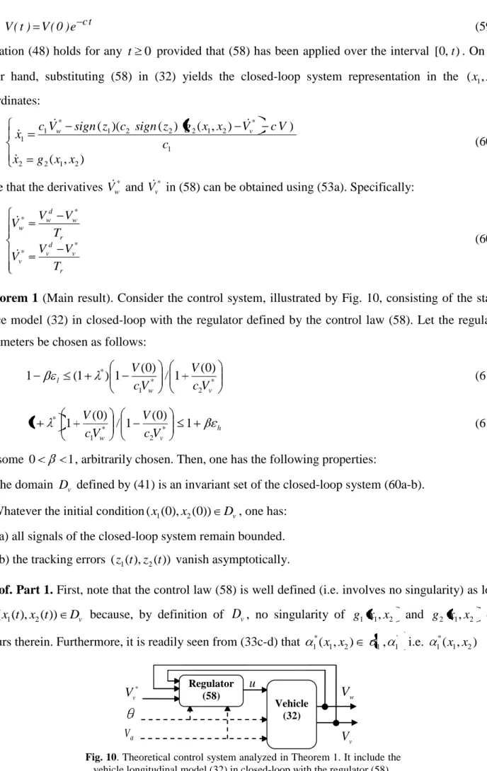
Theorem 1 (Main result). Consider the control system, illustrated by Fig. 10, consisting of the state-space model (32) in closed-loop with the regulator defined by the control law (58). Let the regulator parameters be chosen as follows:

* 2 * 1 * (0) 1 / ) 0 ( 1 ) 1 ( 1 v w l V c V V c V (61a) h v w cV V V c V 1 ) 0 ( 1 / ) 0 ( 1 1 _* 2 * 1 * (61b) for some 0 1, arbitrarily chosen. Then, one has the following properties:

1) The domain D_v defined by (41) is an invariant set of the closed-loop system (60a-b). 2) Whatever the initial condition(x₁(0),x₂(0)) D_v, one has:

a) all signals of the closed-loop system remain bounded. b) the tracking errors (z₁(t),z₂(t)) vanish asymptotically.

Proof.Part 1. First, note that the control law (58) is well defined (i.e. involves no singularity) as long as (x₁(t),x₂(t)) D_v because, by definition of D_v, no singularity of g₁ x₁,x₂ and g₂ x₁,x₂ can occurs therein. Furthermore, it is readily seen from (33c-d) that ₁*(x₁,x₂) ₁, ₁' i.e. ₁*(x₁,x₂)

*

v

V

Fig. 10. Theoretical control system analyzed in Theorem 1. It include the vehicle longitudinal model (32) in closed-loop with the regulator (58)

u v V w V a V Regulator (58) Vehicle (32)

never vanishes. Now, let us show that D_v is an invariant set of the closed-loop system (49a-b). To this end, suppose that (x₁(0),x₂(0)) D_v. As the right sides of (60a-b) are piecewise continuous functions of (x₁,x₂), there exist a 0 such that, for all t (0 ), one has (x₁(t),x₂(t)) D_v which in view of

(41) means that: h l x x 1 1 2 1 _{, for all t [0 ) (62)} h l t _{x t} t x 1 , 1 ) ( ) ( lim 2 1 (63) On the other hand, one gets from (59) that V(t) V(0), for all t [0 ), which together with (56) yields: 2 * 2 2 * 1 * 1 1 * ) 0 ( ) ( ) 0 ( ) 0 ( ) ( ) 0 ( c V V t x c V V c V V t x c V V v v w w , for all t [0 )

This in turn gives:

2 * 1 * 2 1 2 * 1 * ) 0 ( ) 0 ( ) ( ) ( ) 0 ( ) 0 ( c V V c V V t x t x c V V c V V v w v w or, equivalently: * 2 * 1 * * 2 1 * 2 * 1 * * ) 0 ( 1 ) 0 ( 1 ) ( ) ( ) 0 ( 1 ) 0 ( 1 v w v w v w v w V c V V c V V V t x t x V c V V c V V V , for all t [0, ) (64)

Using (53b), it follows from (64) that, for all t [0, ):

* 2 * 1 * 2 1 * 2 * 1 * ) 0 ( 1 ) 0 ( 1 ) 1 ( ) ( ) ( ) 0 ( 1 ) 0 ( 1 ) 1 ( v w v w V c V V c V t x t x V c V V c V

which, together with (61a-b), gives _{l h}

t x t x 1 ) ( ) ( 1 2 1

, for all t [0 ). But, this clearly

contradicts (63) because 0 1. So, D_v is actually an invariant set of the system (60a-b).

Part 2. From Part 1, it follows that if (x₁(0),x₂(0)) D_v then (x₁(t),x₂(t)) D_v, for all t 0. Then,

equation (58)-(59) hold for all t 0. Equation (59) implies that V(t) is bounded and, consequently, so are x1(t) and x2(t), due to (54) and (56). Furthermore, since the right side of (58) is a piecewise

function of (x1,x2) and involves no singularity (because (x1(t),x2(t)) Dv), it follows that the control

signal u(t) is also bounded proving Part 2a. Part 2b is a direct consequence of (59). This completes the proof of Theorem 3.1

Remarks 1. 1) Theorem 3.1 ensures that the closed-loop system is asymptotically stable (in the )

,

(z₁ z₂ -coordinates) with an attraction region containing the whole validity domain D_v.

2) A crucial step in the regulator development was to find out a suitable Lyapunov function. In particular, quadratic like functions turned out to be helpless, due to the particular structure of the controlled system.

3) Inequalities in (61a-b) can easily be fulfilled letting

h h * l 1 and c1,c2 be sufficiently large.

4) Theorem 1 shows that the regulator (58) performs well when applied to the control design model (32). The question is whether such a good performance is preserved when the regulator is applied to the more accurate model (52), see (Figs. 12a). This question is investigated by simulation in Section IV.

3.3.Control Law Design Neglecting Tire Dynamics

Presently, the simplified control design model (38) is based upon. The control objective is to enforce the vehicle speed Vv to follow the reference trajectory

*

v

V . Introduce the control error: * 2 v def V x z (65)

From (41) it is follows that this error undergoes the following equation: * 2) (x Vv f u z  (66)

Consider the Lyapunov function candidate:

2 ) ( 2 z z V (67)

Using (66)-(67), one gets the time-derivative of V(z) with respect to time: * 2) (x V_v f u z V  (68)

This suggests the following control law: z c V x f u _v 2 ) ( 1 * 2  (69)

with c 0 is a design parameter. Indeed, substituting (67) in (68) gives V cV which shows that V is exponentially vanishing. Hence, the control objective (i.e. z 0) is ensured if the control law

(69) is applied to the simplified model (38). The question is whether such a good performance is preserved when the control law (69) is applied to the more realistic model (52) (Fig. 12b). This question is investigated in Section IV.

3.4 Further Discussion on Practical Implementation

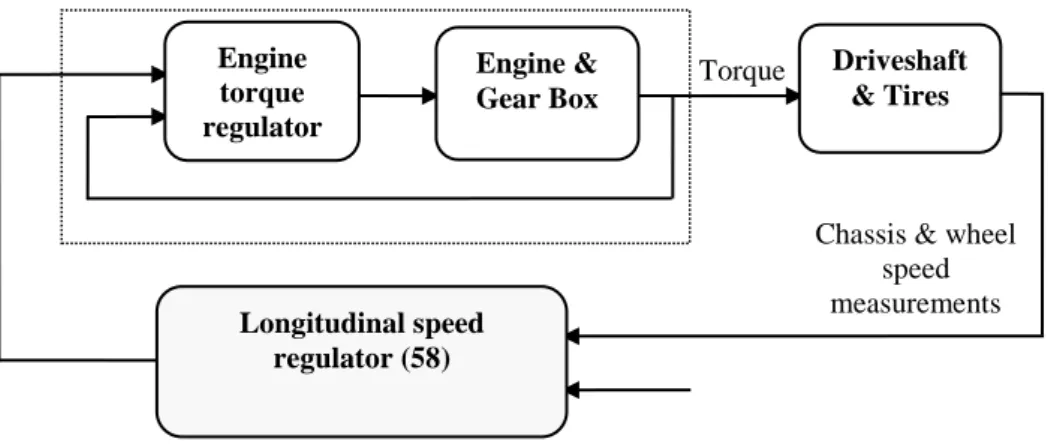
First, notice that the control action generated by a vehicle longitudinal controller (like (58)) constitutes the torque reference signal for the engine torque regulator (not discussed in this study). Accordingly, the longitudinal speed regulator and the engine torque regulator constitute together a more global cascade controller (Fig. 11). In cascade control jargon, the torque regulator is referred to „inner‟ or „slave‟ while the speed regulator is called „outer‟ or „master‟. For the global cascade controller to perform well the torque regulator must be designed so that the inner loop is much more rapid than the outer loop. The previous remarks are independent of the engine technological nature (thermal, electric or hybrid).

Recall also that the analytical design of the (outer) longitudinal speed regulator (58) (developed in Section III) relies on the longitudinal vehicle model (32)-(33). The numerical values of the involved parameters depend on the particular vehicle under study (for instance, Table VI shows those of a Citroën-2CV). They should normally be provided by the vehicle manufacturer; otherwise they must be determined using model identification methods.

The controller design parameters (c,c₁,c₂,T_r) must be given suitable numerical values before online running of the control algorithm. As shown by simulation (Section IV), suitable values can simply be selected following the usual „try-an-error‟ search method.

The practical application of the longitudinal speed regulator necessitates the numerical implementation of the control law (58) and speed measurements (x₁ V_w and x₂ V_v). As the controlled system have

relatively slow dynamics (due to its mechanical nature) a sampling frequency of 100 Hz would be convenient for data acquisition. Following the usual practice, the conditioning of data acquisition is made better if the signals are properly processed before sampling. Online pre-processing operations include signal filtering, amplification, modulation, demodulation etc. Given the simplicity of involved online algebraic operations (in control law and signal processing), the small number of online input/output measurements and the relatively low data-acquisition frequency, the required computation resources are relatively modest. A low-cost DSP and any one of today‟s microprocessors or programmable logic controllers (PLC) would be sufficient for real-time implementation of the control algorithm. The major numerical implementation tasks are described by Table V.

TABLE V. CONTROLLER IMPLEMENTATION ALGORITHM

Step #0# Choice of design parameter and sampling time

Step #1# Acquisition of parameters and states variables x1(k) and x2(k) Step #2# Generate the reference trajectories Vv*(k) and ( )

*

k Vw

Step #3# Compute the control law u(k)

Step #4# Apply the control value to the engine

Step #5# _{Set k k 1and Go to step #1#}

4. SIMULATION

The performances of the sophisticated controller (58), obtained from model (32), will be compared using numerical simulations, to those of the simpler controller (69), obtained from the simpler and less accurate model (38). Both controllers are applied to the most accurate (simulation-oriented) vehicle longitudinal model (52), that not only account for tire dynamics but also for the validity domain (41) so that the model operation is singularity-free. That is, the simulation study will be performed, with Matlab-Simulink, according to the experimental setups illustrated by Figs 12a and 12b, respectively. The characteristics of the vehicle are those of a Citroën-2CV of Table VI.

Fig. 12a. Vehicle longitudinal control involving the simulation-oriented model (52) in closed-loop with the sophisticated speed regulator (58)

Fig. 12a. Vehicle longitudinal control involving the simulation-oriented model (52) in closed-loop with the simpler speed regulator (69)

* v V u v V w V a V Regulator (69) Vehicle model (52) * v V u v V w V a V Regulator (58) Vehicle model (52) Engine & Gear Box Driveshaft & Tires Longitudinal speed regulator (58) Torque Torque reference u

Fig. 11. Global cascade controller for vehicle longitudinal speed control. The grey part refers to the (outer) speed control loop dealt with in the present study.

Engine torque regulator

Chassis & wheel speed measurements

TABLE VI.NUMERICAL CHARACTERISTICS OF THE CITROËN-2CV CAR (FROM CHAIBET,2006)

AD : Asphalt Dry, CW : Cobblestone Wet AD CW

C1 : Primary tire parameter 1.2801 0.5

C2 : Primary tire parameter 23.99 30

C3 : Primary tire parameter 0.52 0.2

Mv : Chassis mass 560 kg

J : Wheel inertia 1000 kg m2

reff : Effective wheel radius 0.28 m

rr : Rolling resistance coefficient 0.025

: Related height of the center of gravity 0.2

: Related position of center of gravity 0.43

Kv : Load correction factor 0.55

: Density of air 1.202 kg/m3

Cx : Aerodynamic drag coefficient 0.5

Cz : Aerodynamic lift coefficient 0.259

S : Frontal area vehicle 0.8 m2

As mentioned previously, there is no simple way to find the best choice for the design parameters i.e.c,c1,c2,Tr. Following the usual practice, suitable numerical values are selected using the heuristic

„try-an-error‟ search method. Accordingly, the next values have been obtained: . the model reference time constant in (53a) is set to Tr 1s,

. the design parameters c,c1,c2 for the controller (58) are given the values c 0.1, c1 60, c2 2,

. the best choice of the design parameter c in the controller (69) turned out to be c 2. 4.1. Control Performances in Easy Driving Conditions

Presently, the control performances of both controllers are illustrated in ideal driving conditions characterized by dry and flat road and weak front wind. Specifically, the driving conditions are defined by the model parameters 0 , V_a 10km/h, (C₁,C₂,C₃) (1.2801,23.89,0.52).

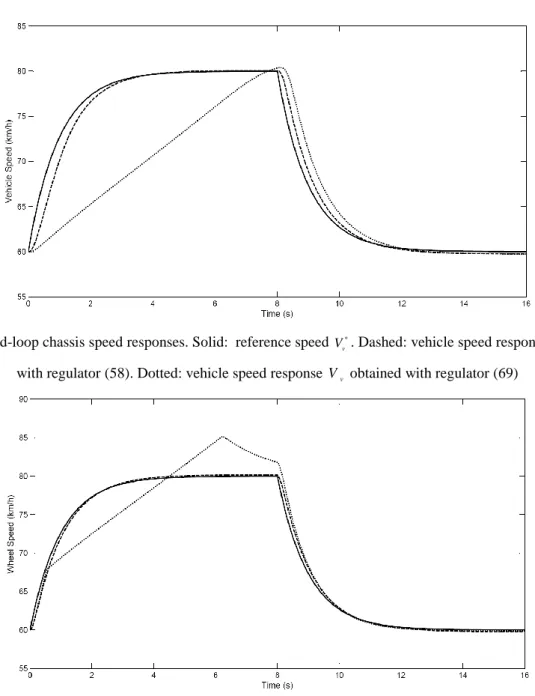
Furthermore, it is supposed that all above values are perfectly known to the designer and used in the controller design. Figs. 13a-e show the control system responses obtained with both controllers in these easy driving conditions. For both, the speed responses, V_v and V_w,converge to their respective references (with settling time less than 1.75s) and present no overshoot in the acceleration mode (Figs. 13a-b). But, as expected, the performances of the sophisticated controller (58) are clearly better than

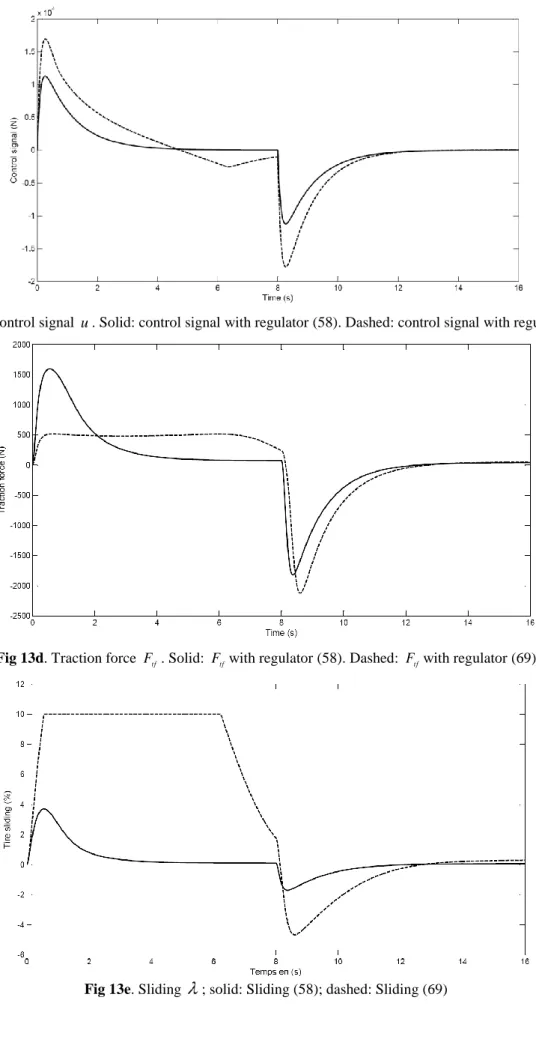
those of (69). Indeed, the former is much more speedier, develops a smaller control effort (Fig. 13c-d) and ensures a weaker sliding (Fig. 13e).

4.2. Control Performances in Hard Driving Conditions

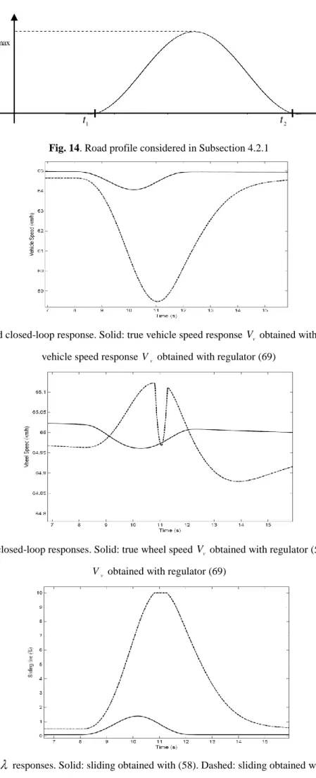
Presently, the driving conditions are much harder compared to the previous subsection. That is, the road is given the profile of Fig. 14 showing an ascendant stage followed immediately by a descent stage. Analytically, the varying road slop is defined as follows:

2 2 1 1 1 2 1 max 0 0 )) 2 cos( 1 ( 2 1 0 ) ( t t for t t t for t t for t t t t t (70)

with _max 10 , t1 8s,t2 12s. Furthermore, the road is Asphalt Dry, characterized by:

(C₁,C₂,C₃) (1.2801,23.99,0.52)

Fig. 15a-b show the vehicle and wheel velocities obtained with both controllers. It is seen that the deviation (between wheel and chassis velocities) gets larger when the vehicle passes over the road bump, between t₁ 8s and t₂ 12s. However, the deviation is much larger with the simpler controller

(69) than with the sophisticated one (58). This fact is better illustrated by Fig. 16 that show the behavior of sliding is better with controller (58).

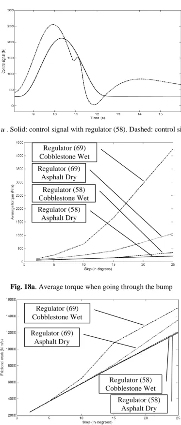
Fig. 17 shows the wheel torque developed by both controllers. Clearly, the regulator (69) develops a huge torque (on the wheel) during the ascendant stage. In the descendant stage, the developed torque decays drastically taking small values. As a matter of fact, such behavior is practically unacceptable because it is harmful for (person and vehicle) safety and is costly from an energetic viewpoint. Clearly, the regulator (58) is better. The supremacy of (58) over (69) is now quantified considering the average torque and frictional work done by the front tires. These are respectively defined as follows:

dt u T_A 0 1 (71) 0 1 dt V F D_{A tf w} (72)

where u is the torque applied to the wheels, F_tf is the component of the frictional force projected onto the tangential direction of the contact surface, V_w is the speed of contact tire-road and is the entire simulation time interval. Fig. 18a shows the variation of the average torque and frictional work with the maximum slop _max. The comparison between the two controllers is dealt with considering two

road states i.e.:

- Cobblestone Wet (C₁,C₂,C₃) (0.5, 30, 0.2).

The figure indicates that, in all driving conditions, the average torque of the vehicle being driven by the regulator (58) is much smaller than with the regulator (69). This confirms that energy consumption is lower with (58) and safety is better. From Fig.18b it is seen that tire friction activity is much weaker when the vehicle is driven with the regulator (58), especially when the vehicle is going through a bump by cobblestone wet road condition. Then, a high tire friction activity is involved with the controller (69) which means that the tires are then subject high pressure.

Fig 13a. Closed-loop chassis speed responses. Solid: reference speed *

v

V . Dashed: vehicle speed response Vv obtained

with regulator (58). Dotted: vehicle speed response V_v obtained with regulator (69)

Fig 13b. Wheel speed responses. Solid: reference d w

V . Dashed: speed response V_wwith regulator (58). Dotted: speed

Fig 13c. Control signal u. Solid: control signal with regulator (58). Dashed: control signal with regulator (69)

Fig 13d. Traction force F_tf. Solid: F_tfwith regulator (58). Dashed: F_tfwith regulator (69)

Fig. 14. Road profile considered in Subsection 4.2.1

Fig. 15a. Vehicle speed closed-loop response. Solid: true vehicle speed response V_v obtained with regulator (58). Dotted: vehicle speed response Vv obtained with regulator (69)

Fig. 15b. Wheel speed closed-loop responses. Solid: true wheel speed Vv obtained with regulator (58). Dotted: wheel speed v

V obtained with regulator (69)

Fig. 16. Sliding responses. Solid: sliding obtained with (58). Dashed: sliding obtained with regulator (69)

1

t t2

Fig. 17. Control signal u. Solid: control signal with regulator (58). Dashed: control signal with regulator (69)

Fig. 18a. Average torque when going through the bump

Fig. 18b. Frictional effort done by the tire

5. CONCLUSION

The problem of vehicle longitudinal control is addressed, both in acceleration and deceleration modes, based on the two new models defined by (32) and (52). The originality of these models lies in the fact that they explicitly accounts for the longitudinal slip (resulting from tire deformation) using Kiencke‟s

Regulator (69) Cobblestone Wet Regulator (69) Asphalt Dry Regulator (58) Cobblestone Wet Regulator (58) Asphalt Dry Regulator (69) Cobblestone Wet Regulator (69) Asphalt Dry Regulator (58) Cobblestone Wet Regulator (58) Asphalt Dry

model. Furthermore, the model (52) also accounts for real-life considerations that physically limit the longitudinal slip value. Consequently, (52) turns out to be quite suitable for simulating the vehicle longitudinal behavior. The control design is based on the slightly simpler model (32) which ignores the slip limitation but still accounts for the tire longitudinal slip. It is shown that a speed controller can actually be obtained from that model using a Lyapunov type design technique. It is formally shown that the obtained controller, defined by (58), does meet its performances i.e. stability and perfect speed reference. It is also checked by simulation that the controller (58) is much better than the simpler one defined by (69) and ignoring longitudinal slip. The supremacy of (58) is especially appreciated in hard driving conditions i.e. crossing rampant and wet roads. In all simulated experiments, the vehicle longitudinal motion is represented by the most accurate and highly nonlinear model (52).

REFERENCES

Chaibet A., (2006). “Contrôle Latéral et Longitudinal pour le Suivi de Véhicule”, PhD, Université d‟Evry Val d‟Essonne, France.

Dugoff P.F.H. and L. Segel, (1970). “An analysis of tire traction properties and their influence on vehicle dynamic performance”, SAE Technical Paper 700377, vol 3, pp. 1219-1243, doi:10.4271/700377.

Gim G. and P. Nikravesh, (1990). “An analytical model of pneumatic tyres for vehicle dynamic simulations part1: Pure slips”, International Journal of Vehicle Design, Vol. 11, No. 6, pp. 589-618. Guo K. and L. Ren, (2000). “A non-steady and non-linear tire model under large lateral slip condition”,

SAE Technical Paper 2000-01-0358, 2000, doi:10.4271/2000-01-0358.

Ioannou P.A. and C.C. Chien, (1993). “Autonomous Intelligent Cruise Control”. IEEE Transactions on Vehicular Technology, Vol. 42, No. 4, pp. 657-672.

Khalil H.K., (2002). “Nonlinear Systems”, Prentice-Hall, 3rd edition.

Kiencke U. and L. Nielsen, (2005). “Automotive control system for engine, driveline, and vehicle”, 2nd edition, Springer.

Liang H., K.T. Chong and T.S. No, S.Y. Yi, (2003). “Vehicle longitudinal brake control using variable parameter sliding control”. Control Engineering Practice, Vol. 11, No. 4, pp. 403-411

Milliken F.W. and L.D. Milliken, “Race car vehicle dynamics”, SAE International, 1995.

Moon S., I. Moon and K. Yi, (2009). “Design, tuning, and evaluation of a full-range adaptive cruise control system with collision avoidance”. Control Engineering Practice, Vol. 17, No. 4, pp. 442-455. Nouvelière L. and S. Mammar, (2007). “Experimental vehicle longitudinal control using a second

order sliding mode”. Control Engineering Practice, Vol. 15, No. 8, pp. 943-954.

Pacejka H.B. and I.J.M. Besselink, (1997). “Magic Formula Tyre Model with Transient Properties”, 2nd International Tyre Colloquium on Tyre Models for Vehicle Dynamic Analysis, Berlin, Germany.

Poursamad A. and M. Montazeri, (2008). “Design of genetic-fuzzy control strategy for parallel hybrid electric vehicles”. Control Engineering Practice, Vol. 16, No. 7, pp. 861-873

Powers W.F. and P.R. Nicastri, (2000). “Automotive vehicle control challenges in the 21st century”. Control Engineering Practice, Vol. 8, pp. 605-618.

Ren T.J., T.C. Chen and C.J. Chen, (2008). “Motion control for a two-wheeled vehicle using a self-tuning PID controller”. Control Engineering Practice, Vol. 16, No. 3, pp. 365-375

Yamakawa J., A. Kojima and K. Watanabe (2007). “A method of torque control for independent wheel drive vehicles on rough terrain”. Journal of Terramechanics, Vol. 44, pp. 371–381.

You S.H., J.O. Hahn and H. Lee, (2009). “New adaptive approaches to real-time estimation of vehicle sideslip angle”. Control Engineering Practice, Vol. 17, No. 12, pp. 1367-1379.