Rapid Prototyping and Exploration Environment for Generating C-to-Hardware-Compilers

R A P I D P R O T O T Y P I N G A N D E X P L O R A T I O N

E N V I R O N M E N T F O R G E N E R A T I N G

C -T O - H A R D WA R E - C O M P I L E R S

e i n g e r e i c h t e d i s s e r tat i o n

vo r g e l e g t z u r e r l a n g u n g d e s g r a d e s

d o k t o r- i n g e n i e u r ( d r . - i n g . )

vo n d i p l . - i n f o r m . f l o r i a n - w o l f g a n g s t o c k au s

b r au n s c h w e i g

Prof. Dr.-Ing. Christian Hochberger Einreichung: 2018-02-05

Prüfung: 2018-03-19

Darmstadt – Februar 2018 D 17

Stock, Florian-Wolfgang :Rapid Prototyping and Exploration Envi-ronment for Generating C-to-Hardware-Compilers

Darmstadt, Technische Universität Darmstadt

Jahr der Veröffentlichung der Dissertation auf TUprints: 2019 Tag der mündlichen Prüfung: 2018-03-19

Veröffentlicht under CC BY-SA 4.0 International

A B S T R A C T

There is today an ever-increasing demand for more computa-tional power coupled with a desire to minimize energy require-ments. Hardware accelerators currently appear to be the best solution to this problem. While general purpose computation with GPUs seem to be very successful in this area, they perform adequately only in those cases where the data access patterns and utilized algorithms fit the underlying architecture. ASICs on the other hand can yield even better results in terms of perfor-mance and energy consumption, but are very inflexible, as they are manufactured with an application specific circuitry. Field Programmable Gate Arrays (FPGAs) represent a combination of approaches: With their application specific hardware they pro-vide high computational power while requiring, for many appli-cations, less energy than a CPU or a GPU. On the other hand they are far more flexible than an ASIC due to their reconfigurability. The only remaining problem is the programming of the FP-GAs, as they are far more difficult to program compared to reg-ular software. To allow common software developers, who have at best very limited knowledge in hardware design, to make use of these devices, tools were developed that take a regular high level language and generate hardware from it.

Among such tools, C-to-HDL compilers are a particularly wide-spread approach. These compilers attempt to translate common C code into a hardware description language from which a dat-apath is generated. Most of these compilers have many restric-tions for the input and differ in their underlying generated micro architecture, their scheduling method, their applied optimiza-tions, their execution model and even their target hardware. Thus, a comparison of a certain aspect alone, like their implemented scheduling method or their generated micro architecture, is al-most impossible, as they differ in so many other aspects.

This work provides a survey of the existing C-to-HDL compil-ers and presents a new approach to evaluating and exploring dif-ferent micro architectures for dynamic scheduling used by such compilers. From a mathematically formulated rule set the Triad compiler generates a backend for theScalecompiler framework, which then implements a hardware generation backend with de-scribed dynamic scheduling.

While more than a factor of four slower than hardware from highly optimized compilers, this environment allows easy com-parison and exploration of different rule sets and the micro archi-tecture for the dynamically scheduled datapaths generated from them. For demonstration purposes a rule set modeling the CO-COMAtoken flow model from theCOMRADE 2.0compiler was implemented. Multiple variants of it were explored: Savings of up to 11 % of the required hardware resources were possible.

Z U S A M M E N FA S S U N G

Heutzutage gibt es eine immer größere Nachfrage nach mehr Rechenleistung, bei gleichzeitigem Wunsch immer weniger En-ergie dafür aufzuwenden. Momentan sind Hardwarebeschleu-niger die beste Lösung hierfür. Während GPUs in diesem Ge-biet sehr erfolgreich sind, bringen sie ihre beste Leistung nur zur Geltung, wenn die Algorithmen und Speicherzugriffsmuster auf die zugrundeliegende Architektur abgestimmt sind. Anderseits können ASICs noch mehr Leistung bei noch geringerem Energie-verbrauch zur Verfügung stellen, sind aber aufgrund ihrer fest-gelegten Funktionalität sehr unflexibel. Eine Kombination aus beiden Ansätzen sind FPGAs: Sie können bei hoher Energieeffi-zienz eine große Rechenleistung zur Verfügung stellen, sind aber gleichzeitig durch ihre Rekonfigurierbarkeit flexibler als ASICs. Ein offenes Problem ist aber immer noch die Programmierung der FPGAs, da sie viel schwerer zu programmieren sind als her-kömmliche Software. Eine mögliche Lösung hierfür sind C-to-HDL Compiler, die herkömmlichen C Code in eine Hardware-beschreibungssprache übersetzen, um daraus Hardware zu ge-nerieren. Viele von diesen Compilern haben Einschränkungen was den unterstützten Sprachumfang angeht, und unterschei-den sich in unterschei-den verwendeten Optimierungen, der Ablaufplanung, der generierten Mikroarchitektur, ihrem Ausführungsmodell oder der Zielhardware. Diese vielen Unterschiede machen einen Vergleich bezüglich nur eines Aspektes fast unmöglich.

Diese Arbeit bietet eine in die Breite gehende Übersicht über die existierenden C-to-HDL Compiler und stellt ein System vor, das eine schnelle Evaluierung verschiedener Ansätze zur dyna-mischen Ablaufplanung ermöglicht. Hierzu liest der Compiler-generatorTriadeinen formalen Satz Regeln ein, aus denen dann ein Compilerbackend für das CompilerframeworkScalegeneriert wird, das C in eine Hardwarebeschreibungsprache übersetzen kann. Die erzeugte Hardware nutzt dabei eine dynamische Ab-laufplanung, die durch den formalen Regelsatz definiert wurde. Während die generierte Hardware mehr als viermal langsa-mer ist, als die von spezialisierten optimierenden Compilern, er-laubt die vorgestellte Umgebung das schnellere Ausprobieren von verschiedensten Ansätze. Zu Demonstrationszwecken wur-de im Regelsatz die Ablaufplanung vomCOMRADE 2.0

Compi-ler nachgebildet. Mit nur wenig Aufwand wurde eine Variante erkundet, welche bei Tests bis zu 11% weniger Hardware Res-sourcen benötigt.

DA N K S A G U N G

Hello, Hello – this is dedicated to the ones I love.

Edgar —Electric Dreams, 1984

Ein erster Stelle möchte ich meinem Doktorvater Prof. Dr.-Ing Andreas Koch danken, der mich immer gut unterstützt hat. So-wohl bei wissenschaftlichen als auch bei nicht-wissenschaftlichen Themen war er immer eine Hilfe und hat mich angetrieben als es nötig war.

Außerdem möchte ich Prof. Dr.-Ing. Christian Hochberger für das kurzfristige Erstellen des Zweitgutachtens danken.

Tobias Riepe habe ich, neben Andreas, für die vielen sprachli-chen Verbesserungsvorschläge zu danken.

Mein größter Dank gilt meiner Familie für die Unterstützung. Insbesondere meiner Frau, die mehr Geduld mit mir hatte, als jede(r) Andere und immer für mich da war.

C O N T E N T S

Acronyms and Abbreviations xv

1 i n t r o d u c t i o n 1 1.1 ACS 4 1.2 Challenges 5 1.3 Thesis 6 2 f o u n dat i o n s 9 2.1 Compiler 9 2.1.1 Control Flow 10

2.2 High Level Synthesis 19

2.2.1 Scheduling 20

2.2.2 Allocation and Binding 21

2.2.3 Generating Hardware from High Level Lan-guages 24 3 p r i o r w o r k 35 3.1 Evolution of HW-Compilers 35 3.2 Survey of C-to-HDL-Compilers 38 3.2.1 Typology 39 3.2.2 Overview 43

3.3 COMRADEandCOCOMA 43

3.3.1 COMRADE 44

3.3.2 COCOMA 49

3.3.3 Module Libraries 49

3.4 TheScalecompiler framework 56

3.4.1 hardScaleCompiler 59

4 c -t o - h d l - c o m p i l e r g e n e r at o r t r i a d 61

4.1 Ideas and Concepts 62

4.2 Triad 63 4.2.1 Hardware Operators 63 4.2.2 Operator Mapping 66 4.2.3 Scheduling Rules 69 4.2.4 Token Specification 70 4.2.5 Entity Selection 72 4.2.6 Guard Condition 73 4.2.7 Action 75 4.2.8 Macros 77

x c o n t e n t s

4.2.9 Simple Token Based Scheduling 77

4.2.10 Requirements and Limitations 81

4.2.11 Implementation 82

4.3 GeneratedhardScaleBackend 83

5 e va l uat i o n 99

5.1 Implementation ofCOCOMA-based Rule Set 99

5.2 Testcases and Environment 103

5.3 Synthesis Results 105

5.4 Token Model Variants 106

5.5 Optimization 107 6 s u m m a r y a n d f u t u r e w o r k 109 a f o r m a l d e f i n i t i o n s 111 b l i s t o f c -t o - h d l - c o m p i l e r s 115 b.1 xPilot 115 b.2 Bach-C 116 b.3 C2H 116

b.4 Altera SDK for OpenCL 117

b.5 C2R 117 b.6 C2Verilog 118 b.7 Carte 119 b.8 Cascade 120 b.9 CASH 120 b.10 Catapult-C 122 b.11 CHC 122 b.12 CHiMPS 123 b.13 COSYMA 123 b.14 CToVerilog 124 b.15 Comrade 125 b.16 CVC 125 b.17 Cyber 126 b.18 Daedalus 126 b.19 DIME-C 127 b.20 eXCite 127 b.21 FP-Compiler 128 b.22 FPGA C 128 b.23 GarpCC 129 b.24 GAUT 130 b.25 GCC2Verilog 130 b.26 Handel-C 131 b.27 Hthreads 131

c o n t e n t s xi b.28 Impulse-C 132 b.29 LegUp 133 b.30 Mitrion-C 133 b.31 Napa C 134 b.32 Nimble 134 b.33 NYMBLE 135 b.34 Bambu 135 b.35 PICO-Express 135 b.36 PRISC 136

b.37 ROCCC (Riverside Optimizing Compiler for Con-figurable Computing) 137 b.38 SPARK 137 b.39 Trident 138 b.40 XPP-VC 138 b.41 DWARV 139 c t r i a d s y n ta x 141 c.1 EBNF 141 c.2 Syntax Diagrams 145 d t r i a d f i l e 149

d.1 COCOMADynamicCancelTokens Rules 149

d.2 COCOMAStaticCancelTokens Rules 153

b i b l i o g r a p h y 155

Own Publications 179

L I S T O F F I G U R E S

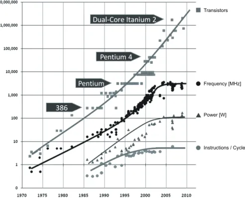
Figure 1.1 CPU frequencies and transistor count 1

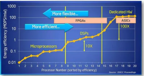
Figure 1.2 CPU, FPGA, and DSP comparison 3

Figure 2.1 Compiler phases from the gcc Compiler 9

Figure 2.2 Example of different IRs 11

Figure 2.3 Examples of control flow frames 12

Figure 2.4 C-Program and its CFG 13

Figure 2.5 t-structured C program 14

Figure 2.6 Subgraph containing a loop that is t-structured. 15

Figure 2.7 Transformation from code into SSA form. 16

Figure 2.8 𝜙function in SSA-form 16

Figure 2.9 Conversion out-of SSA form 17

Figure 2.10 DFG 17

Figure 2.11 CDFG 18

Figure 2.12 Memory Dependence 18

Figure 2.13 Flow for generating hardware. 19

Figure 2.14 DFG for complex multiplication 22

Figure 2.15 Binding example 22

Figure 2.16 Scheduling example 23

Figure 2.17 Scheduling example (improved) 23

Figure 2.18 Virtex 7 Slice 25

Figure 2.19 C Code 27

Figure 2.20 HW-SW callbacks 30

Figure 2.21 Transforming control into data flow 31

Figure 2.22 Alias analysis 33

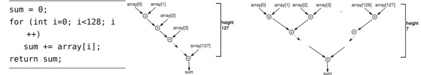
Figure 2.23 Tree height reduction 33

Figure 3.1 Sales of synthesis tools 36

Figure 3.2 AccelDSP and BlueSpec Comparison 39

Figure 3.3 COMRADESW Service 46

Figure 3.4 Speculative execution inCOMRADE 47

Figure 3.5 ACE-V Platform 48

Figure 3.6 COMRADE 2.0Compile Flow 50

Figure 3.7 modlibModule Library 51

Figure 3.8 COMRADEClass Diagram 54

Figure 3.9 GAPScreenshot 56

Figure 3.10 VeriDebugScreenshot 56

Figure 3.11 pnnsGraphScreenshot 57

Figure 3.12 ScaleDataflow 58

Figure 4.1 TriadandScaleInteraction 62

Figure 4.2 Triadmodule definition 64

Figure 4.3 Triadexpression to hw module mapping 66

Figure 4.4 Different Token Sets 71

Figure 4.5 Token Based Scheduling 78

Figure 4.6 Control Flow in Simple Model 80

Figure 4.7 InternalTriadFlow 82

Figure 4.8 ScribbleCFG 87

Figure 4.9 TriadGenerated CDFG 89

Figure 4.10 Operator Wrapper 91

Figure 4.11 Very Simple Datapath 91

Figure 5.1 COCOMARules (Legend) 100

Figure 5.2 COCOMARules 101

Figure 5.3 Memory requirements for the testcases. 103

Figure 5.4 Standard COCOMAtoken flow with dy-namiccanceltokens compared to static can-celtoken waiting at the multiplexer. Run-time did not change. 106

Figure 5.5 Comparison of required resources from data path with and without token logic. 107

Figure 5.6 Reducing the token logic induced logic over-head by treating subgraphs as virtual op-erators. 108

Figure B.1 SRC Computers SRC-7 MAPstation 119

Figure B.2 PegasusIR 121

Figure B.3 PICO system-level architecture 136

L I S T O F T A B L E S

Table 3.1 HLS Evaluation Criterias 40

Table 3.2 Comparison ofNIMBLE,COMRADE, and COMRADE 2.0. 44

Table 3.3 modlibParameters 52

Table 3.4 NecessaryCOMRADEcompiler passes. 55

Table 4.1 Optional Hardware Operations 64

Table 4.2 ScaleExpressions 68

Table 4.3 Entities inTriad 73

Table 4.4 Predicates inTriad. 75

Table 4.6 Token Controller Example 94

Table 4.7 Token Controller Example 95

Table 4.8 Token Controller Example 95

Table 5.1 Benchmark Characteristic 104

Table 5.2 Synthesis results for the CHStone testcases. 105

L I S T I N G S

Listing 2.1 C-Program: Factorial Example 11

Listing 2.2 gccGimple IR 11

Listing 2.3 gccRTL IR 11

Listing 2.4 LLVMIR 11

Listing 2.5 RAW Dependency 18

Listing 2.6 WAR Dependency 18

Listing 2.7 WAW Dependency 18

Listing 4.1 Example of aTriadfile,HWOPS-section. 65

Listing 4.2 Scale expression to hardware module map-ping for addition. 67

Listing 4.3 Example rule in Triad. 70

Listing 4.4 Token Specification 71

Listing 4.5 Example Rule inTriad 76

Listing 4.6 Macros inTriad 77

Listing 4.7 Triadrules section for scheduling pure data flow with anactivatetoken. 79

Listing 4.8 Generated wrapper module. 84

Listing 4.9 Generated Java code for instantiation of anaddmodule. 85

Listing 4.10 HW Selection Pragmas 86

Listing 4.11 TriadVisitor excerpt. 88

Listing 4.12 Pseudocode for the hardware generation in the backend. 90

Listing 4.13 Pseudocode for the token controller gen-eration from rules. 93

ac r o n y m s xv

A C R O N Y M S A N D A B B R E V I A T I O N S

ACS Adaptive Computing System ALU Arithmetic-Logic-Units ASAP As-soon-as-possible

ASIC Application Specific Integrated Circuit ASIC Application Specific Integrated Circuits AST Abstract Syntax Tree

AT activatetokens BB Basic Block

Behaviour Description Language BDL CDFG Control Data Flow Graph CDFG Control Data Flow Graph CFF Control Flow Frame CFG Control Flow Graphs CLB Configurable Logic Block

CMDFG Control Memory Data Flow Graph

COCOMA COMRADE Controller Micro-Architecture COINS COmpiler INfraStructure

CPLD Complex Programmable Logic Devices CPU Central Processing Units

CSP Communicating Sequential Processes CT canceltokens

CTL CHiMPS target language DF Dominance Frontier DFG Data Flow Graph

xvi ac r o n y m s a n d a b b r e v i at i o n s

DFGs Data Flow Graphs

DSL Domain Specific Language DSP Digital Signal Processor EBNF Extended Backus-Naur Form Event-Condition-Action ECA

FPGA Field Programmable Gate Array FSB Front Side Bus

FSM Finite State Machine

GPGPU General Purpose Graphic Processing Unit HDL Hardware Description Language

HLL High Level Language HLS High Level Synthesis

HPC High Performance Computing HW hardware

ILP Integer Linear Programming IO Input-/Output IR Intermediate Representation KPN Kahn-Process-Networks KPN Kahn-Process-Networks LB Loop Body LP Linear Program LSQ Load Store Queue LUT Look Up Table MUX Multiplexer

PDF Post-Dominance Frontier RC Reconfigurable Computing

ac r o n y m s a n d a b b r e v i at i o n s xvii

RCU RC unit

RTL Register Transfer Language RTL Register Transfer Logic RTL Register-Transfer-Logic

Scale Scalable Compiler for Analytical Experiments SIMD Single Instruction Multiple Data

SSA Static Single Assignment STL Standard Template Library t-structured top-structured

1

[…]it’s my opinion that anyone who can possibly introduce science to the nonscientist should do so.

I S A A C A S I M O V – Interview, 1980 Ongoing advances in computer technology allow for smaller and smaller manufacturing process sizes.

More and more transistors per area are available (as forecast by Moore’s Law [135]) but despite the fact that Central Process-ing Units (CPU) utilize them, the top clock frequencies of them have stagnated since the mid-2000s around the 4 GHz mark (see Figure1.1).

While some approaches use a smaller transistor size to keep the number of transistors constant, and fit the circuit into a smaller

Instructions /Cycle Power[W] Frequency [MHz] Transistors

Figure 1.1: Development of clock frequencies and transistor count of conventional CPUs (data from K. Olukotun, Intel).

2 i n t r o d u c t i o n

area, resulting a higher yield and lower power consumption, most approaches try to accelerate computations by utilizing the higher number of available transistors.

Recent approaches to utilize the higher number of the avail-able logic resources concentrate mostly on

• bigger caches,

• multiple functional units, including multi- and many-core approaches as well as vector units, and

• dedicated task specific logic (for example encryption or video acceleration). Depending on the size, this could be just a small part of a chip, dedicated to one task, or even an own chip (Application Specific Integrated Circuit (ASIC)). If more processing power is required, the first approach is no viable solution. Since computation time is an order of magni-tude faster than memory access time, caches are used to hide the latencies by caching the data in faster, local memories. Thus bigger caches can improve memory bottlenecks in certain cases, but not in all of them. In particular, a single task does not ben-efit any more from further increased cache size after a certain, task-specific, limit is reached.

Replicating functional logic blocks works very well when the processor has to handle multiple tasks in parallel. Accelerating just a single task is only possible when the problem can be di-vided into multiple parts which can actually run independently from each other and thus utilize the replicated logic. This is en-tirely dependent on the input program, and in reality it ranges from problems that behave very nicely and allow for partitioning into very many parallel parts, to the other end of the spectrum with problems that are purely sequential and do not allow for parallel execution at all. A good example for the first group of problems are almost all math problems involving matrices and vectors, where operations are performed column-/element-wise independently from the other columns/elements. The modern cryptographic hash function scrypt [149] is an example of a function that was explicitly constructed to allow no parallelism in order to reduce the attack surface for brute force attacks.

In general Amdahl’s Law [10] describes the upper limit of how beneficial parallelism can be (for example, a program which al-lows 50% of it to be executed on 2 units while the rest is limited to sequential execution, gains at most a speed up of 25% from parallelization).

i n t r o d u c t i o n 3

Figure 1.2: CPU, FPGA, and DSP comparison

Standard CPUs try to use the program’s inherent parallelism via replication of small functional units (for example multiple load-store-units, vector instructions). Other problem-specific processors can maximize this by replicating complete smaller processors. For example, General Purpose Graphic Processing Unit (GPGPU) have hundreds of processors working on the same problem in parallel, usually in a Single Instruction Multi-ple Data (SIMD) design. Even though these units provide huge amounts of computational power (NVIDIA Tesla V100 has up to 30.0 TFLOPS [50]) this approach suffers from the lack of gen-erality as not all problems can be mapped to the computation model of these GPGPUs.

Therefore, the third approach is the most viable when trying to accelerate a generic single task: Use hardware (HW) that is tailored to that specific task. The drawback with common dedi-cated task specific logic is, that it is dedidedi-cated. It is hardwired to its specific task. In case of changing tasks the hardware wastes just the area resources in best case, while in the worst case also power is wasted as well.

A solution to this is reconfigurable hardware. While not as fast as dedicated logic, it is usually faster than an all purpose CPU (but not as flexible, see Figure1.2).

To get the best of both worlds; flexibility of a CPU, efficiency of an ASIC – one combines a regular CPU with reconfigurable hardware as accelerator. Such a combination is called an Adap-tive Computing System (ACS).

4 i n t r o d u c t i o n

1.1 ac s

In an ACS reconfigurable logic, usually in form of a Field Pro-grammable Gate Array (FPGA), is combined with a conven-tional CPU.

FPGAs consist of very regular logic building blocks that are connected via routing resources. Building blocks that can im-plement different logic functions (usually via a Look Up Table (LUT)) and configurable switches connecting them allow the FPGA to realize almost arbitrarily complex logic functions. As mentioned above , ongoing miniaturization allows for more and more such blocks, and the trend is to use the high available num-ber of transistors for more complex logic blocks ( like complete Digital Signal Processing (DSP)-blocks). The commercial FPGA market is dominated by two big companies, Xilinx and Altera (has been owned by Intel since 2015).

Both offer FPGA series that contain a complete standard CPU as building block. Xilinx started in their old Virtex-4FX/-5FX series [196, 197] with an embedded PowerPC 405/440 hard-core and continued this trend with ARM dual-hard-core Cortex-A9 in Zynq-7000 series and ARM quad-core Cortex-A53 in the newest Zynq UltraScale series[198].

Altera had an ARM v4 in their older Excalibur series of FP-GAs [46], and have, similar to Xilinx, an ARM Cortex-A9 in their newest Arria and Cyclone [48,49]) series.

On those models the CPU is on the same die as the FPGA, which allows a very fast on chip bus connection between both.

Such a close connection between FPGA and CPU is not neces-sary for an ACS; other architectures are possible, but the slower the communication between both is, the faster the FPGA must be to compensate for the data transfer overhead to generate a speedup.

At the moment solutions with connections on every level exist. From the FPGA CPU combination mentioned above, which use an on chip bus, to systems that use faster system buses between different dies within one package (for example Intel QuickAssist QPI FPGA Platform uses QPI links [40]) and system buses be-tween different chips (e.g. Convey uses the Intel Front Side Bus (FSB) [42,43]). The slowest variant are periphery buses (for ex-ample an FPGA card with PCI Express).

The connection between both is one factor that impacts the ac-celeration, while the other important factor is the memory model

1.2 c h a l l e n g e s 5

(memory bandwidth, shared memory, cache coherence, virtual-ization, …).

Such ACS already have shown their usefulness at a multitude of different applications, for example

• Cray built 2004 their entry level High Performance Com-puting (HPC) machine XD1 as ACS. An XD1 Rack consists of 12 chassis, each holding 12 64-bit AMD Opteron 200 CPUs accompanied with 6 Virtex II-Pro FPGAs [100]. • Convey/Micron built the HPC ACS systems 𝐻𝐶 − 1 and

𝐻𝐶 − 1𝑒𝑥. A standard Intel Xeon CPU is coupled via FSB to 4 Xilinx Virtex 5 (in 𝐻𝐶 − 1) / Virtex 6 (in 𝐻𝐶 − 1𝑒𝑥) FPGAs using a cache-coherent NUMA architecture. In the latest Convey generation the FPGA is coupled to the CPU via PCIe [42,43].

• The HARP (and HARP 2) program from Intel, which intro-duces theIntel QuickAssist QPI FPGA Platform. On this plat-form an Intel XEON-CPU is coupled with an Altera FPGA via QPI and packaged together [40].

1.2 c h a l l e n g e s

When using ACS new problems appear, namely:

• Communication between FPGA and CPU can be so expen-sive that all time gained by the acceleration from the FPGA is lost through Input-/Output (IO). Faster signaling can help here ([118]).

• The shared memory must be handled with care. Especially cache coherency must be considered.

• For optimal performance, the task has to be partitioned into a part that can be accelerated on the FPGA and a part that remains on the CPU. This partitioning problem, which has to split the program into those two parts, and mod-eling the communication from the chosen architecture as constraints, is from a theoretical viewpoint NP-hard. So-lutions can use good heuristics (e.g. Kerninghan-Lin algo-rithm [128], genetic algorithms [59], simulated annealing or tabu search [61]), as well as exact solver (e.g. via Integer Linear Programming (ILP) [141, 142], branch-and-bound [21,127] or dynamic programming [126]). Often this step

6 i n t r o d u c t i o n

is avoided by requiring the programmer to manually de-cide which parts of the program have to be accelerated on the FPGA.

• The implementation of the reconfigurable logic in a Hard-ware Description Language (HDL).

The description of a synthesizable logic circuit in a HDL is quite different from programming in a conventional (procedu-ral, functional or object orientated) language. It requires much more knowledge and experience and is very error prone.

To allow common software developers to develop for the ACS, the hardware description must be hidden from them. This prob-lem is not specific to ACS; in pure HW development it is desir-able to move away from low level HDLs to more abstract lan-guages as well. Easing the programming and debugging for soft-ware developers and giving them the capability to develop HW is not the only benefit of this approach; a higher abstraction level also allows for faster turn around times for HW developers.

Besides extensions to standard HDLs to increase the level of abstraction (e.g. SystemVerilog), translating high level lan-guages into HDL became a common approach (for more on these topics see Section3.1).

To translate legacy code and make a high-level-to-HDL-compiler usable for as many software programmers as possi-ble, it would be desirable to choose a widespread language as a source language. According to different statistical sources ( [169, 190]) one of the most important and popular languages is still C ([111]). Only Java can compete with its popularity, but C is, due to its much simpler language constructs, much more suitable for translation into a HDL.

1.3 t h e s i s

In the Embedded Systems and Applications Group of the TU Darmstadt several different high-level-to-HDL-compilers were used and developed. Different research projects had different fo-cuses, ranging from different input languages and different exe-cution models of the generated hardware, via different compiler internals, to different memory architectures and much more.

Working with them and experimenting with different setups was (and still is) very tedious and trying to evaluate several micro architectures is often impossible, because the different projects often use different compilers and compiler frameworks.

1.3 t h e s i s 7

Often it is only guesswork why two approaches yield different re-sults, as one cannot trace back the different results to differences in used compilers, compiler settings, compiler optimizations, compiler internals, generated micro architecture, used hardware, environment or scheduling of the code.

The contribution of this thesis is to provide a system that al-lows the analysis and comparison of different micro architec-tures without the need to reimplement them completely anew in a common environment. To allow this, a framework is devel-oped which is able to generate different C-to-HDL compilers, which have a common base but only differ in their HW gener-ating backends, and hence allow an unbiased comparison.

The C-to-HDL compilers are generated from a formal descrip-tion. This description is so versatile that it allows easy explo-ration of different architectures and concepts.

Not only can the compiler back ends be easily explored, but ex-plorations and adaptions to the common compiler environments can be instantly applied to all existing generated variants by generation of the compiler, as well. This allows, for example, re-search of the impact of new compiler optimizations on different HW back ends.

The thesis is structured as follows:

First, the definitions and fundamentals used are introduced in Chapter2.

Secondly, Chapter 3 will give a broad overview over prior and related work. An (non-exhaustive) survey of C-to-HDL-Compiler is done and they are classified according to a proposed taxonomy.

Although, the developed Compiler framework is independent from the C-to-HDL-Compiler COMRADE, it was one major mo-tivation and it is analyzed in more detail.

In Chapter 4 the Domain Specific Language (DSL) used for the formal description is introduced and its implementation is described.

Afterwards the generated compilers are evaluated, together with the compiler generator itself, in Chapter5.

Finally, the work is concluded with a summary and an outlook in Chapter6.

2

Everything of any importance is founded on mathematics.

Jonny Rico –Starship Troopers, R O B E R T A . H E I N L E I N, 1959 As laid out in the introduction, the focus of this work is about the development of C-to-HDL-compilers. One of the goals of those compilers was to abstract the hardware, so software de-velopers can use them. In consequence this means, that build-ing such compilers requires knowledge from both worlds, hard-ware and softhard-ware. Hence, this foundations section is divided into three parts. First, the software part: this is basically about compilers. The second part is about hardware generation and fi-nally: co-execution of hardware and software, which is necessary when hardware should run as accelerator. In this chapter the used terms, formalism, and fundamentals for these three parts are defined. Most of the information in this section is just com-mon text book knowledge, so an exhaustive list of references for them is omitted and only references to some of them are given ([1, 56, 110, 136]). The explanation of the terms is kept concise; the formal definitions are collected in AppendixA.

2.1 c o m p i l e r

The typical compiler is split into three parts: front end, middle end, and back end. Usually the front end scans and parses the input, the middle end performs optimizations and the back end generates the output. The Intermediate Representation (IR) is

Front End Middle End Back End

GIMPLE

AST RTL

C _{lexing &} ASM

parsing

optimizations

10 f o u n dat i o n s

the internal data representation the compiler uses between dif-ferent steps. Figure2.1shows a compiler having all three phases and using different IRs.

Several IRs are possible, some compilers even have multiple IRs, depending on the required level of abstraction (for example see [41,121,170]).

An often used IR is an abstract, assembler-like language. De-pending on the intended optimizations and tasks, the abstrac-tion level can vary. An example for a very abstract IR is LLVMs IR, which has, similar to a Turing machine, infinitely many regis-ters. An example for a less abstract IR is the GCC Register Trans-fer Language (RTL) which is very close to the target machines assembler code. Figure2.2shows some examples of such IRs.

An often used data structure for IRs is the graph. These are commonly (additionally) used, especially for hardware com-pilers, to represent control flow Control Flow Graphs (CFG) and/or the flow of data in the program Data Flow Graphs (DFGs). The graph representation allows an easy combination of both pieces of information or the addition of other informa-tion in form of addiinforma-tional edges or nodes or annotainforma-tions to them. A common enhancement are additional edges for memory de-pendencies. In the next sections these common graph IRs are ex-plained.

2.1.1 Control Flow

The general idea behind a CFG, is that the program is modeled as graph, where the nodes correspond to the statements and op-erations in the program and the edges model the sequence of the possible execution order. The detailed formal definition is in AppendixA.

The non-branching blocks of code that become nodes are called Basic Blocks (BB) (see Definition1).

Now we need to model the possible flow of execution, es-pecially the possible branches. This is done with Control Flow Frames (CFF) (see Definition2), which allows us to model the control flow in programs with a dedicated start and end node. A function𝑐𝑜𝑛𝑑is necessary to annotate edges of branches with the result of the condition. A special value 𝜖is used to annotate de-fault cases in switch statements and as value for non-branching edges.

2.1 c o m p i l e r 11

int fak(int c) {

if (c == 1)

return 1;

else

return c * fak(c-1);

}

(a) Original C-Code

fak (int c) { int D.1798; if (c == 1) goto <D.1796>; else goto <D.1797>; <D.1796>: D.1798 = 1; return D.1798; <D.1797>: _1 = c + -1; _2 = fak (_1); D.1798 = c * _2; return D.1798; }

(b) High level GIMPLE IR from GCC

(insn/f 33 32 34 2 (set (reg/f:DI 6 bp)

(reg/f:DI 7 sp)) "fak.c":1 81 {*movdi_internal} (nil))

(insn/f 34 33 35 2 (parallel [ (set (reg/f:DI 7 sp)

(plus:DI (reg/f:DI 7 sp)

(const_int -16 [0xfffffffffffffff0]))) (clobber (reg:CC 17 flags))

(clobber (mem:BLK (scratch) [0 A8]))

]) "fak.c":1 984 {pro_epilogue_adjust_stack_di_add} (c) Low level GCC RTL (excerpt)

; Function Attrs: noinline nounwind uwtable define i32 @fak(i32) #0 {

[...]

; <label>:7:

%8 = load i32, i32* %3, align 4 %9 = load i32, i32* %3, align 4 %10 = sub nsw i32 %9, 1

%11 = call i32 @fak(i32 %10) %12 = mul nsw i32 %8, %11 store i32 %12, i32* %2, align 4 br label %13

[...]

(d) LLVM IR

Figure 2.2: Example of different IRs for the standardfactorialexample code.

12 f o u n dat i o n s Start A 0 B 1 End ε ε Start A 1 B 2 C 3 D ε ε ε End ε ε

Figure 2.3: Examples of control flow frames (if and switch) Figure 2.3 shows two graphical examples of two CFFs repre-senting a single for and a single switch statement. In general they can be almost arbitrarily complex.

With the CFF supplying the structure of the graph, the addi-tion of BB as nodes gives a complete graph, which models the complete program. This resulting graph is calledCFG(see Defi-nition3).

For compiler optimizations and transformations that operate on the CFG, it is useful to define some terms which occur again and again to ease the description of the algorithms:

A branch node (see Definition 4) is a node where the control flow splits, and at a join node (see Definition 5) the previously split flow joins again. A subset of nodes is called a region (see Definition 6). A dominator (see Definitions 7 and 9) of a node is every node that must lie along the path from the start node to itself. Similar apost-dominatorof a node (see Definitions8and10) is every node that must lay along the path from the node itself to the end node. A node 𝑛1controls(see Definition11) another

node𝑛₂, if𝑛₂ is executed after𝑛₁and 𝑛₁decides whether𝑛₂ is executed or not.

2.1 c o m p i l e r 13

int main() {

int i;

printf(”The loop starts . . . \ n”);

for (i = 0; i < 5; i++) printf(”Hello World!\n”); printf(”The loop has ended!\n”);

return 0; } main () loop 1 FREQ:0 <bb 4>: if (i <= 4) goto <bb 3>; else goto <bb 5>; FREQ:0 <bb 3>:

__builtin_puts (&"Hello World!"[0]); i = i + 1;

[0%]

FREQ:0 <bb 5>:

__builtin_puts (&"The loop has ended!"[0]); D.1838 = 0; [0%] [0%] ENTRY EXIT FREQ:0 <bb 2>:

__builtin_puts (&"The loop starts..."[0]); i = 0; goto <bb 4>; [0%] [0%] FREQ:0 <bb 6>: <L3>: return D.1838; [0%] [0%]

Figure 2.4: C-Program and the generated corresponding CFG. Figure 2.4shows a simple C program together with the CFG that represents this program. For graphical representation dif-ferent degrees of detail are possible, such as giving the detailed statements of the BB in the nodes when required, or just label-ing the nodes with a unique identifier when just the structure is relevant. In the given example each gray block represents a basic block, which is identified by a sequential number within the<bb

>tag.

The above terms can all be found within the small example: b r a n c h n o d e : The only basic block that is a branch node is

<bb 4>. It is after the check of the loop end condition, where the control flow can either branch to the next loop iteration or to the next instruction after the loop.

14 f o u n dat i o n s

(a)

int func(int a) {

int s; s = 0; l1: s += a; a--; if (a != 0) goto l1: return s; } (b)

int func(int a) {

int s; s = 0; do { s += a; a--; } while (a != 0) ; return s; } (c)

int func(int a) {

int s; s = 0; s += a; a--; while (a != 0) { s += a; a--; } return s; }

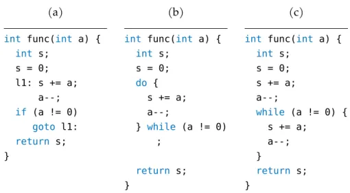
Figure 2.5: C program with gotos (a), transformed into a structured C program (b), and into a t-structured C program (c). j o i n n o d e : <bb 4> is also the join node. Before the check of

the loop condition the control flows of the pre-loop code and in case of repeated loop iteration join.

r e g i o n : As a region is just a subset, multiple regions are present, for example <bb 4> and <bb 5>make up a re-gion (in Figure2.4boxed and labeled withloop 1). d o m i n at e s r e l at i o n : An example for domination would be

<bb 2>, as it dominates every other node (i.e. it must be executed before).

p o s t- d o m i n at e s r e l at i o n : Similarly <bb 6> post-dominates every other node.

( p o s t- ) d o m i n a n c e f r o n t i e r : For node <bb 3> the post dominance frontier would contain only the node<bb 4>. In this case it would be also its dominance frontier.

c o n t r o l d e p e n d e n c e : <bb 4>controls<bb 3>.

When handling different input languages, different patterns are generated in the resulting CFG. If the input is restricted to structured imperative programming languages the result-ing graphs have some advantageous properties. Structured pro-grams are all imperative propro-grams that have no explicit or im-plicit goto (break, continue, exception or similar) statements and are just a concatenation, selection or repetition of instructions

2.1 c o m p i l e r 15

A !cond

subgraph condε

Figure 2.6: Subgraph containing a loop that is t-structured. or subprograms. All common C programs can be transformed via goto removal into such a structured program [23,64]. As a further simplification the structured program can be normalized into a top-structured (t-structured) program (see Definition12). This consists only of loops that are evaluating the loop condition at the top, and not at the bottom.

The C programming language has just a do-while-loop with evaluation at the bottom, which can be easily transformed into a functional equivalent while-loop (see Figure2.5for such trans-formations).

Such t-structured programs have the useful property that each node of the CFG has at most one controlling node [67]. When generating a hardware description for the program this simpli-fies the task, as the translation/generation is limited to one kind of loop.

For later discussion we also introduce the following terms: Back edge(see Definition13), loop header (see Definition14), and loop body (see Definition15).

Another advantageous property often used is the Static Sin-gle Assignment (SSA) form [53] (see Definition 16), which de-mands that each variable is defined only in one place. This prop-erty is not limited to CFGs, but can also be applied to all other IRs that contain assignments. It not only simplifies and improves many optimizations but is also advantageous for the hardware generation, as every data has exactly one single point of defini-tion.

It is easy to transform arbitrary code into code that fulfills the first condition of the definition: Every time a variable is written after its first definition in the code, the variable is renamed into a new one. Of course all subsequent accesses have to be corrected to use the new name. A common technique is to use the same

16 f o u n dat i o n s x = x + y; y = x + y; z = x + y; x₁ = x₀ + y₀; y₁ = x₁ + y₀; z₀ = x₁ + y₁;

Figure 2.7: Transformation from code into SSA form. x = ... if (cond) x = x + y; z = x + y; x₀ = ... if (cond) x₁ = x₀ + y₀; z₀ = x_? + y₁; x₀ = ... if (cond) x₁ = x₀ + y₀; x₂ = 𝜙 (x₀, x₁); z₀ = x₂ + y₁;

Figure 2.8: Regular C-Code, its SSA form without𝜙function (depend-ing on the condition the𝑥_?must be either𝑥₁or𝑥₂), and its SSA form with𝜙function.

variable name with an index (version number) for each defini-tion. Figure2.7shows such a renaming.

The second property of the definition demands that after join-ing different code paths, both of which redefine the variable, a new, unique variable is created which can be used to access the current value afterwards, regardless of which branch was taken. Therefore, a function is introduced that selects one of its argu-ments, depending on the control flow that led to its execution. This function is called𝜙-function. In Figure2.8 an example for the use of this𝜙-function is shown.

As no CPU physically supports such a function, all compilers which emit assembler code must remove these𝜙-functions. This process is often calledconversion out-of SSA formordestruction of SSA form, even when it is afterwards still has the SSA property.

During the conversion the versioned variables are kept, and appropriate copy instructions are inserted in the different con-trol flows before the 𝜙-function. Figure 2.9 shows the example SSA form from Figure2.8after such a destruction. This example is trivial but in general, with more complex control flows, it can get quite complicated. An often used approach is the algorithm from Briggs et al. [25], which improves the algorithm originally presented [53].

2.1.1.1 Data Flow

Data flow models go back to the 1960s. They were introduced to model the flow of data items through a network. Various similar

2.1 c o m p i l e r 17 x₀ = ... if (cond) x₁ = x₀ + y₀; x₂ = x₁ else x₂ = x₀ z₀ = x₂ + y₁;

Figure 2.9: Example code from Figure 2.8converted out-of SSA form (unoptimized) . c = b*a; d = c+d; e = a*c - b*d; a b d e * + -* *

Figure 2.10: Example for the DFG representation of C-Code. models, some super-sets of others, were proposed. Some are still in widespread use, like Petri Nets ([138]), computation graphs ([106]), or Kahn Process Networks ([105]).

Similar to the CFG, the data flow is also modeled as a graph, but in this case it is a directed acyclic graph. The nodes repre-sent operators, while the edges model the flow of the data items between the operators.

Figure2.10gives an example of a DFG and the C code it repre-sents. The elegant modeling of the creation of data, its consump-tion and the flow between operaconsump-tions is not only used inside com-pilers. It can also be used to represent Register-Transfer-Logic (RTL), which is used to describe synchronous hardware circuits. Even complete architectures have been designed on the data flow model ([82]).

In this simple form control flow cannot be handled, only a sin-gle basic block can be represented by a DFG. One way to include control flow would be to combine CFG and DFG representations into a Control Data Flow Graph (CDFG), where special edges are inserted into the DFG to represent the control dependencies (Figure2.11shows such a graph).

18 f o u n dat i o n s c = b*a; if (c > 0) d = c+d; else d = c-d; e = a*c - b*d; a b d e * + -* * ->0

Figure 2.11: Example for the CDFG representation of C-Code.

a = b + c; d = a + c;

(a) Read after write (RAW) depen-dency

a = b + c; b = c + d;

(b) Write after read (WAR) depen-dency

c = a + b; c = d + e;

(c) Write after write (WAW) depen-dency

Figure 2.12: Examples for memory dependency (assuming that each variable access is actually a memory access).

2.1.1.2 Memory Dependence

The focus of the COMRADE compiler[67] (more details in Sec-tion3.3) was the Control Memory Data Flow Graph (CMDFG). These further advancement to CDFGs adds another type of edge, that is added between two nodes, describing memory accesses (read or write) when there is a dependency between those.

Memory accesses that are independent from each other have the advantage, that they can be executed in parallel or out-of-order.

Figure 2.12 shows the three kind of dependencies that exist. When in one of the cases (in listing (a) variable a, in (b)b, and in (c) c) the execution order is changed, a wrong value is read or written, invalidating the computation.

These cases are very easily to detect, far more problematic are the cases, when the access happen not via a constant ref-erence, but with an arbitrary pointer, where the address is not known at compile time. When no other information is available, the compiler must assume the worst case and treat them as

de-2.2 h i g h l e v e l s y n t h e s i s 19

Behavioral Level

Register Transfer Level

Level of Abstraction

Physical Level Technology Level

Logic Level

Transformation

Scheduling, Allocation, Binding

State Encoding, Logic Synthesis

Technology Mapping

Place & Route

Figure 2.13: Flow for generating hardware.

pendent, presumably degrading the performance. Besides using hints from the programmer (the C language introduced for this reason the restrict keyword in theC99 standard) many com-pilers try to improve the situation by trying to proof that two pointers do not refer to the same position (see Section2.2.3.4).

In theCOCOMAfromCOMRADEsCMDFG[67] the memory edges are not only used to model the memory dependencies be-tween the memory accesses, but also to serialize them. Having only one memory backend port, the accesses to them must be ordered somehow. Using memory edges between a memory ac-cess and the next one in program order fulfills this task.

2.2 h i g h l e v e l s y n t h e s i s

Hardware generation in general is a long and complex process. Figure2.13shows the most important steps involved when build-ing digital circuits.

The first step, the transformation from the behavioral level to a structural description on the RTL, is called High Level Synthe-sis (HLS) [133]. Starting with a behavioral description (usually in an HDL like Verilog, VHDL, Chisel or Bluespec) of what the hardware is supposed to do, the level of abstraction is lowered with different transformations. Each of the transformations leads to a lower level of abstraction, with the transformations being: Allocation, binding and scheduling. As these are part of almost all HLS compilers, they are explained in greater detail in the sec-tions below. The other steps happen after the HLS by specialized programs/tools, so just a concise explanation is given; for a more detailed description see [133,153].

s tat e e n c o d i n g Generates a Finite State Machine (FSM) and the encoding for the required states when necessary.

20 f o u n dat i o n s

l o g i c s y n t h e s i s The RTL description gets translated into an logic-level representation (which is usually a netlist). Also includes a minimization/optimization of the generated logic.

t e c h n o l o g y m a p p i n g Process of mapping generic logic functions to the specific functions available in the technol-ogy used.

p l ac e & r o u t e In this step the available objects in the tech-nology get physically placed and connected. Both are very complex, and each of it alone is NP-complete ([73,74]). Even when listed separatly, several of them are highly depen-dent on each other; especially, those that are shown on the same level in Figure2.13are often executed together. This applies even more to the transformations of the HLS step. These phases are highly intermingled: Each decision made in one phase has an impact on subsequent phases. For example if two operations are scheduled on the same time step, they cannot be bound to the same resource. Decisions which seem optimal for a phase can degrade the result quality of a later phase. As there is (so far) no per se perfect ordering of the phases, the problem is known as phase order problemor phase coupling problem. Most hardware synthesis systems apply the scheduling first, then allocation and binding, but other approaches have also been tried [166]. Some perform binding and allocation before scheduling, others try to combine scheduling, allocation and binding into a single phase (e.g. with ILP formulations) [133].

2.2.1 Scheduling

The starting time of each operation is determined in such a way that all constraints are met. There are as simple algorithms as As-soon-as-possible (ASAP) scheduling, which schedules an opera-tion as soon as the constrains allow it. But there are also more so-phisticated schemes, like the often used List Scheduler. For HLL compilers the used scheduling algorithms can be classified in one of three groups, depending on when and how the schedul-ing happens:

s tat i c The exact fixed starting times are determined com-pletely by the scheduling algorithm (like the above men-tioned ASAP or List scheduler) at compile-/design-time.

2.2 h i g h l e v e l s y n t h e s i s 21

d y n a m i c The necessary timings are not computed statically at compile-/design-time, but the necessary decisions when an operation has to be started are made at run-time. m i x e d Sometimes also referred as quasi-static, this is a

combi-nation of static and dynamic scheduling, where some of the scheduling decisions are made at run-time and some at compile-/design-time.

For the small example problem the operations are just se-quentially executed. But with more complex computations the scheduling of the operations is far more critical as this can im-pact the latency of the whole computation.

2.2.2 Allocation and Binding

In the allocation step it is defined which resources will be used in the final circuit. During the binding step the mapping from the operations to the allocated resources happens.

As both steps depend on each other (only allocated resources can be bound on one hand, on the other it makes only sense to allocate resources that become bound later), they are performed together in one phase.

This is more complex than it seems, as there is not necessar-ily a one-to-one mapping from the operations to the hardware resources. A resource could be shared between different usages, it could even perform different operations (for example an ALU can do different computations). For operations the concrete im-plementation must be chosen (many operations allow different implementations which trade area for speed).

In general this is an optimization problem which usually aims at minimizing the used resources and/or the required glue logic and wiring, or more concretely the used area. Like many other problems in the hardware generation flow this problem is NP-complete, so different heuristics are used to solve it[166].

Example

As an example for the three HLS tasks a complex multiplication (𝑎 + 𝑏𝑖) ∗ (𝑐 + 𝑑𝑖) = 𝑒 + 𝑓 𝑖is used. Figure2.14shows the DFG for this computation. To make the allocation not too trivial, limited resources are assumed: only two multipliers, one adder, and one adder/subtractor are available and are assigned as in Figure2.15.

22 f o u n dat i o n s a * * c * b * d -e + f

Figure 2.14: DFG for the complex multiplication(𝑎 + 𝑏𝑖) ∗ (𝑐 + 𝑑𝑖) = 𝑒 + 𝑓 𝑖. a multiplier_1 multiplier_1 c multiplier_2 b multiplier_2 d adder_subtractor_1 e adder_subtractor_1 f

Figure 2.15: Binding of 2 multiplier, 1 adder, and 1 subtractor to the DFG from Figure2.14.

After the allocation and binding an ASAP scheduling is per-formed. The algorithm is quite simple: Nodes are inserted in topological order of the dependency graph into the first possi-ble time slot, so that a) the previous nodes are finished, and b) the required resources are available.

In the example the order of the nodes is multiplier_1(with inputs from𝑎and𝑐), multiplier_1(𝑎, 𝑑),

multiplier_2(𝑐, 𝑏), multiplier_2(𝑑, 𝑏), adder_subtractor_1(−), adder_subtractor_1(+).

The first multiplication bymultiplier_1(with inputs from𝑎 and𝑑) can be scheduled on time slot 1 without problems. While a second multiplication can be allocated on the other multiplier, the third multiplication is allocated tomultiplier_1too. So this multiplication is scheduled on time slot 2 (for the sake of

sim-2.2 h i g h l e v e l s y n t h e s i s 23 a c d b multiplier_1 multiplier_1 Time slot 1 2 3 4 multiplier_2 multiplier_2 adder_subtractor_1 e adder_subtractor_1 f

Figure 2.16: Schedule from the operations from Figure2.15. plicity of the example it is just assumed that all operations take one time step).

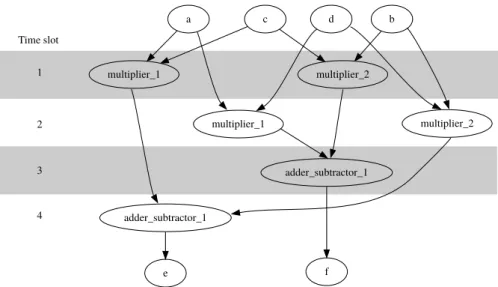
In the same waymultiplier_2got placed on time slots 1 and 2. Theadder_subtractor_1depends on the last scheduled mul-tipliers and so the first operation is scheduled on time slot 3, and the last afterwards on time slot 4. The resulting schedule is de-picted in Figure2.16.

The ASAP schedule is not the perfect solution even in this small example. Figure 2.17 switches the insertion of the multi-plier operations onmultiplier_1and as a consequence the com-putation finishes one time slot earlier.

a c d b multiplier_1 multiplier_1 Time slot 1 2 3 multiplier_2 multiplier_2 adder_subtractor_1 e adder_subtractor_1 f

24 f o u n dat i o n s

2.2.3 Generating Hardware from High Level Languages

Automated hardware generation from a higher level of abstrac-tion, such as a regular programming language, is possible in a number of ways. The most common way is to perform the HLS steps and lower the abstract high level language to an HDL. This way, everything which is close to hardware and dependent on the actual technology used (e.g. logic synthesis, mapping, place and route) is dealt with by the regular tool flow tools.

Despite the most common approach, it is not the only one. Two other ways are:

1. Use libraries in the HLL and use those to perform steps in the hardware generation process below the HLS. One ex-ample for this is theJBitslibrary from Xilinx for Virtex 2 Pro [193–195]). It enables the programmer to write the config-uration bitstream for a reconfigurable device directly and gives him direct control over the used hardware resources and even placing and routing.

2. Generate microcode for a generated/selected application specific or configurable processor. The hardware genera-tion is reduced to selecgenera-tion, configuragenera-tion, and program-ming of a processor (an example for this kind would be PICO[108]).

Chapter 3 and Appendix B list different compilers and the methods used for hardware generation more detailed.

This work takes the same approach as most of the other com-pilers and the compiler generator creates comcom-pilers that generate hardware by emitting Verilog HDL code.

2.2.3.1 Target Hardware

While HLS can target any kind of hardware, the most com-mon application is to generate hardware descriptions for recon-figurable hardware(in opposite to Application Specific Integrated Circuits (ASIC)).

The main element of Reconfigurable Computing (RC) is a hardware element whose functions can be reconfigured, a config-urable device. Most widespread devices that allow such a recon-figuration are Complex Programmable Logic Devices (CPLD)s and the similarly constructed, but bigger and more complex FP-GAs.

2.2 h i g h l e v e l s y n t h e s i s 25

(a) Schematic FPGA (b) Aslice(a CLB has 2 of these) of a Xilinx Virtex 7

Figure 2.18: Xilinx FPGA (source Xilinx).

These consist of different configurable elements which can be connected in different ways. Configurable elements not only in-clude computational or logic elements but also I/O elements and memory.

Depending on the granularity of the device, the size of the computational reconfigurable element changes. Coarse grained devices can have complete Arithmetic-Logic-Units (ALU)s as computing elements (an example for a coarse grained architec-ture is PACT XPP[15]). On the other hand fine grained devices contain LUTs and/or multiplexers as the smallest logic element. The LUT can be configured as arbitrary𝑛-input binary function. Depending on the vendor and the technology used𝑛is usually 4 or 6 (the two vendors with the greatest market share Altera and Xilinx use this approach). Figure 2.18 shows such a mod-ern, newest generation FPGA from Xilinx, a Xilinx Ultrascale. The biggest models have up several hundreds of thousands of Configurable Logic Block (CLB)s, each containing 8 LUTs and 16 flip-flops. Furthermore, they have tens of Megabits of config-urable RAM blocks, thousands of DSP hard blocks and several hard blocks for I/O (for example Ethernet, PCIe, Interlaken)1. Some models even include multiple ARM CPU hard blocks. Ar-ranged in a regular grid between these configurable elements are channels that contain the routing resources. The wires can

26 f o u n dat i o n s

be configured to connect to the logic and as to how they connect with each other to route the nets. For clock signals dedicated net-works are available as well as clock management resources.

The reconfigurability of the device comes at a price: While ASICs can clock up to several GHz, the newest generation FP-GAs are much slower. The above mentioned UltraScale FPGA has as a maximum frequency 𝑓_𝑚𝑎𝑥 for its element of 525 - 741 MHz (depending on the type of element and speed grade of the device) [199]. While there are devices that have persistent con-figuration memory (for example ACTELs Flash-based FPGAs), most of the bigger devices are SRAM based. This means they are no instant-on devices, as the configuration must be read before operation, and they struggle with the same problems as SRAM; esp., they are sensitive to ionizing radiation [173].

While not reaching the frequencies of an ASIC, the FPGA can still accelerate many computations compared to a CPU due to application specific hardware acceleration. Additionally, the re-configuration allows for a change of the implemented hardware afterwards (for example to changing standards or protocols, or when an error is found), and for short development cycles while developing hardware. When the total number of produced units is small, the FPGAs are also much cheaper than an ASIC.

While RC can accelerate computations, an RC unit (RCU) is very inefficient when handling general-purpose applications. The typical application spends most of their time in a small com-putational part, while the rest are I/O and management tasks, which are handled very well by modern CPUs.

The solution is the hybrid approach already mentioned in Chapter 1, called ACS, that consists of a standard CPU, for the administrative tasks, accompanied by an RCU, that handles the compute intense parts. This combination is so popular that the FPGAs do not need to be paired up with an external CPU2, that the manufacturers offer FPGAs with CPU cores (and CPUs with FPGA-fabric).

The main drawback for the ACS is the knowledge required on the programmer’s side. Despite using an HDL, the development of hardware is different from plain software programming. At this point the HLS-compiler is supposed to bridge the knowl-edge gap for the software developer so he can utilize the RCU without expert HW design knowledge. At least that is the hope; in reality there are many problems.

2 or the CPU with an external FPGA, depending on the fact if you see the whole system FPGA-centric or CPU-centric

2.2 h i g h l e v e l s y n t h e s i s 27

if (a+c > b) c = a*b;

else

d = c/d;

Figure 2.19: The hardware version of this high level code requires +, * and / operator, but never * and / simultaneously.

2.2.3.2 Difficulties

So far, the flow for generating hardware from a high level lan-guage presented seems fairly easy: translate it into an HDL, and let the HDL compiler (and other tools) handle the complicated tasks from there. From a theoretical point-of-view the problem that arises is, that the RTL synthesizeable subset from the HDL is not Turing-complete. It can be used for describing netlists, like in XML for describing Turing-complete hardware, but it is itself not Turing-complete. Translating one structured high level lan-guage into another is usually done by replacing each lanlan-guage construct (sequential execution, loop, conditional execution, …) with the corresponding construct of the target language. HDLs are not structured, and due to this mismatch, the translation of the high level language into the low level HDL is not easy. For in-stance, neither the subprogram mechanism (in a modern sense, where arbitrary calls are allowed) nor does the loop construct available in almost every high level language does exist in HDLs. Instead of writing a loop itself, a circuit which will later imple-ment the loop and dedicated control logic has to be created. This process is a complex process, even for one loop, but with nested loops this gets increasingly more complex.

Several compilers avoid this problem by just translating the innermost loop. The computation inside this innermost loop is translated into a data path, and the generated hardware is used as a streaming kernel3(for example [120] uses this approach).

Another drawback is that the hardware which should be equivalent to a software program has to supply all possibly nec-essary functions, even when not all are neededed at all times (or not need at all). It is just not possible to remove one subroutine

3 Streaming is a parallel computation paradigm, where data is considered to be a stream of data and the computation is performed on each of the data ele-ments. No further allocation or communication besides thestreamis required, and usually pipelined hardware profit from this approach, as the pipeline is kept filled by the stream.

28 f o u n dat i o n s

(or parts thereof) in hardware and replace it with a different one. Self reconfiguration would allow this, but no HDL assumes or supports it.

Thus, in many cases complete programs cannot be imple-mented in hardware. One solution is to keep the program as a software program on a CPU, and just accelerate speed critical routines in hardware (these routines are often called kernels). The controlling software on the CPU manages in- and output and configures that kernel onto the FPGA that is required for the current program (ACS).

This execution in hardware and software together is called Hardware-Software-Co-Execution (HW-SW-Coexecution). It leads to another NP-complete problem: the partitioning.

2.2.3.3 Hard- and Software Co-Execution

In an environment where hardware and software are executed together, the program must bepartitioned. This is the process of selecting which parts of the software are executed in hardware and which stay on the CPU.

The most important task is to identify the part of the program which should be moved to the accelerator. Usually, only com-pute intense parts are handled by the accelerator, parts which require limited computation or are I/O-intensive are kept on the CPU. The reason for this is that the specific hardware is often not capable of performing those operations efficiently or cannot do it at all (e.g. system-calls or other I/O-tasks).

Due to the NP-completeness of the problem, many different approaches have been implemented, which are also heavily in-fluenced by the target architecture and computation model.

The different approaches can vary in several aspects, namely: g r a n u l a r i t y Depending on the architecture and the

avail-able size for the generated hardware the granularity of the accelerated part can vary from a single instruction to com-plete programs.

m a n ua l v s au t o m at i c The method for identification of the parts which may and/or should be run in hardware. Many systems rely on manual annotation in the high level code, few try to automatically decide which parts become hard-ware. Most automatic approaches use some kind of profil-ing, where test runs are made in software only. While per-forming these runs, execution information (such as branch

2.2 h i g h l e v e l s y n t h e s i s 29

probabilities, memory access patterns, problem sizes, ex-ecution times) is collected. Using a mathematical model, which takes configuration times, data transfer times be-tween RCU and CPU, estimated and available hardware ar-eas, and the collected data into account, the relevant parts are identified.

c h o o s e b e t w e e n h w a n d s w e x e c u t i o n The decision whether the generated hardware accelerator should be used can be dynamic or static. In the static case it is always used (not using it is also an option, but then why it was generated in the first place?), but in the dynamic case the decision, is made at runtime. The software still contains the necessary software instructions for the generated hard-ware, and depending on several parameters, it is possible that the software version is executed, and the hardware is not used. It is also possible that both versions are run ini-tially, and in later executions only the faster one gets se-lected.

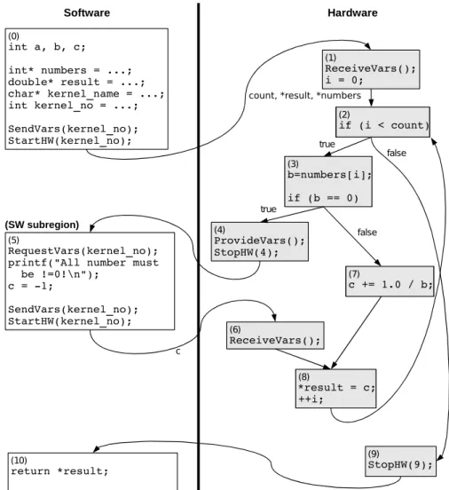
c o n t r o l f l o w t r a n s i t i o n h w- s w Several systems al-low only the CPU to start a computation on the RCU and expect the result later. This approach excludes all software that is not computation-only from acceleration. Even the simplest I/O, even when it is not supposed to happen reg-ularly, prevents the routine from getting implemented in hardware, as the hardware cannot execute it. Figure 2.20

gives an example for such a scenario. More sophisticated systems allow the hardware to pause and perform soft-ware callbacks to execute the system- or I/O-functions ([107]).

a r e a A hard limitation for the generated hardware is set by the available resources on the target reconfigurable device. While most approaches try to gain as much benefit as possi-ble by using as much hardware as possipossi-ble, some go even a step further. They do not only partition into CPU and RCU parts, but also perform temporal partitioning ([188]). This works best with algorithms that have different phases, which are executed sequentially.

The list of HDL compilers in AppendixBcontains more details and references on the partitioning methods used by them.

30 f o u n dat i o n s

double inverseSum(int count, int* numbers) { double result = 0.0;

for (int i = 0; i < count; i++) { if (numbers[i] == 0) {

printf("All numbers must be != 0!\n"); return -1.0; } result += 1.0/numbers[i]; } return result; }

Figure 2.20: The printf, only intended for error handling, stops this code from becoming hardware in most systems, that allow only SW-HW invocation.

2.2.3.4 Hardware Generation and Optimizations

In this section the most common compiler optimizations for HLS-compiler are explained. While many optimizations are use-ful (that is profitable) for all kind of (HLS-)compilers, some are dependent on the micro architecture that the compiler creates for the RCU. The existing compilers can be categorized in three groups of micro architectures:

1. The first group uses a processor that gets programmed in microcode as micro architecture. Usually, this contains also a unit or combination of units that are tailored to the compiled program. For example, this can be an ALU with problem specific bitwidths, vector units with many ele-ments, specific Very Large Instruction Word (VLIW) cores, or more complex units (like FFTs-kernel) that are selected from the input application.

2. The second group generates a static scheduled data path. This can be easily generated from a DFG. This only works when the program contains no control flow. When control flow is supported, this is either handled by removing the control flow before when possible (see below), or by using a FSMs. In the later case eachBasic Blockis translated into a separate DFG, with the FSM orchestrating their activation.

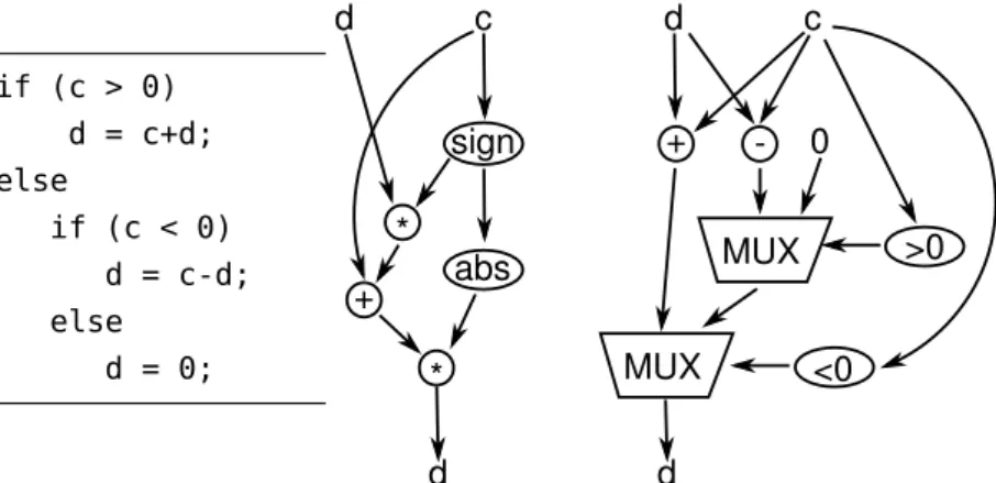
2.2 h i g h l e v e l s y n t h e s i s 31 if (c > 0) d = c+d; else if (c < 0) d = c-d; else d = 0; c d * + abs sign * d >0 <0 0 MUX MUX d c d +

-Figure 2.21: Control flow for computing the expression of the variable dcan be transformed into a data path. This can happen by inserting multiplexers or by mathematical reformulation of the computation intod=abs(sign(c))*(c+sign(c)*d). 3. The third group uses a dynamic runtime scheduling for

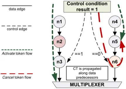
the generated data path. They are not activated by a static schedule, but dynamically. Each of the operators is ac-tivated at run time via signals, often called tokens. The term token came from the models of computation these group implements, which are often graphs or networks of operators where tokens flow along the edges and acti-vate the operations. Two of the most often-used models of computation are Petri-Nets ([138,150]) and Kahn-Process-Networks (KPN) [105, 145]). This scheduling also works with CDFGs and tokens can be used to model the control flow.

The first group can be treated and translated like a CPU. It is actually not really a C-to-HDL compiler, but more a custom-CPU-selector/configurator and a cross-compiler. Therefore, the rest of the discussion excludes these and only includes the last two groups.

r e m o v i n g c o n t r o l f l o w To reduce the complexity of han-dling control flow, it can in some cases be reduced to data flow. This is possible when branching leads just to different computa-tions of the same expression and the value can be selected with an inserted Multiplexer (MUX) or by reformulating the expres-sion. Figure2.21shows an example of C code containing control flow that can be turned into data flow.