Fingerprinting the Smart Home: Detection of Smart Assistants Based on Network Activity

FINGERPRINTING THE SMART HOME: DETECTION OF SMART ASSISTANTS BASED ON NETWORK ACTIVITY

A Thesis presented to

the Faculty of California Polytechnic State University, San Luis Obispo

In Partial Fulfillment

of the Requirements for the Degree Master of Science in Electrical Engineering

by

Arshan Hashemi December 2018

© 2018 Arshan Hashemi ALL RIGHTS RESERVED

COMMITTEE MEMBERSHIP

TITLE: Fingerprinting the Smart Home: Detection of Smart Assistants Based on Network Ac-tivity

AUTHOR: Arshan Hashemi

DATE SUBMITTED: December 2018

COMMITTEE CHAIR: Zachary Peterson, Ph.D.

Associate Professor of Computer Science

COMMITTEE MEMBER: Bridget Benson, Ph.D.

Associate Professor of Electrical Engineering

COMMITTEE MEMBER: John Oliver, Ph.D.

ABSTRACT

Fingerprinting the Smart Home: Detection of Smart Assistants Based on Network Activity

Arshan Hashemi

As the concept of the Smart Home is being embraced globally, IoT devices such as the Amazon Echo, Google Home, and Nest Thermostat are becoming a part of more and more households. In the data-driven world we live in today, internet service providers (ISPs) and companies are collecting large amounts of data and using it to learn about their customers. As a result, it is becoming increasingly important to understand what information ISPs are capable of collecting. IoT devices in particular exhibit distinct behavior patterns and specific functionality which make them especially likely to reveal sensitive information. Collection of this data provides valuable information and can have some serious privacy implications.

In this work I present an approach to fingerprinting IoT devices behind private networks while only examining last-mile internet traffic . Not only does this attack only rely on traffic that would be available to an ISP, it does not require changes to existing infrastructure. Further, it does not rely on packet contents, and therefore works despite encryption.

Using a database of 64 million packets logged over 15 weeks I was able to train machine learning models to classify the Amazon Echo Dot, Amazon Echo Show, Eufy Genie, and Google Home consistently. This approach combines unsupervised and supervised learning and achieves a precision of 99.95%, equating to one false positive per 2,000 predictions. Finally, I discuss the implication of identifying devices within a home.

ACKNOWLEDGMENTS

Thanks to:

• My parents for their continuous love and support.

• Neal Nguyen and Ryan Frawley who’s work constructing the IoT testbed was invaluable to my Thesis

TABLE OF CONTENTS Page LIST OF TABLES . . . ix LIST OF FIGURES . . . xi CHAPTER 1 Introduction . . . 1 2 Related Work . . . 4

2.1 IoT Security and Privacy . . . 4

2.2 Privacy Policies and Practices of Intelligent Virtual Assistants . . . . 4

2.3 Traffic Analysis and Device Fingerprinting . . . 5

2.4 Fingerprinting NATed Hosts and Netflows . . . 6

2.5 Fingerprinting IoT Devices . . . 7

3 Background . . . 9

3.1 IoT and the Smart Home . . . 9

3.2 IVA . . . 9 3.3 Machine Learning . . . 11 3.4 Decision Trees . . . 11 3.5 Random Forests . . . 13 3.6 Neural Networks . . . 15 3.7 K-means clustering . . . 17 3.8 Mini-Batch K-Means . . . 18 3.9 Model Validation . . . 18

3.9.1 K-fold Cross Validation . . . 19

3.10 Classifier Performance Metrics . . . 19

3.10.1 Accuracy . . . 20

3.10.2 Precision . . . 20

3.10.3 Recall . . . 20

3.10.4 F1 Score . . . 21

3.10.5 False Positive Rate . . . 21

3.10.7 One-vs.-Rest Transformation . . . 21 3.11 Clustering Performance . . . 22 3.12 Information Entropy . . . 23 3.13 Tools . . . 24 3.13.1 Matlab . . . 24 3.13.2 Scikit-Learn . . . 24 3.13.3 Bro . . . 24 3.13.4 Wireshark . . . 25 3.13.5 Intel NUC . . . 25 4 The Dataset . . . 26 4.1 Threat Model . . . 26 4.2 IoT Testbed . . . 27

4.3 Implementation of a pipeline for data processing . . . 27

4.3.1 Connection State . . . 28

4.3.2 History . . . 30

4.4 CTU Dataset . . . 30

5 Machine Learning . . . 32

5.1 Methodology . . . 32

5.2 Selection of Machine Learning Algorithms . . . 32

5.3 Feature Selection . . . 33

5.4 Defining Performance Goals . . . 34

5.5 Types of Device Behaviors . . . 35

5.6 Clustering . . . 36

5.7 Classifier Integration . . . 38

5.8 Removing Noise from the Dataset . . . 39

5.9 Note about the Dataset . . . 39

6 Results . . . 40

6.1 Models . . . 40

6.2 Baselines . . . 41

6.3 Experiment 1: K-Means Clustering . . . 42

6.4 Experiment 2: Introducing the Filter . . . 45

6.5.1 Model 1 . . . 51

6.5.2 Model 2 . . . 52

6.5.3 Model 3 . . . 52

6.6 Experiment 4: Realistic Private Network Scenario . . . 54

7 Discussion . . . 56 8 Conclusion . . . 59 BIBLIOGRAPHY . . . 60 APPENDICES A Traffic Analysis . . . 65 B Model Selection . . . 70

B.1 Feedforward Neural Network (MLP) . . . 70

B.2 Random Forests . . . 70

C Feature Selection . . . 73

LIST OF TABLES

Table Page

4.1 Features extracted from each connection . . . 29

4.2 Connection State . . . 29

4.3 Connection History . . . 30

6.1 Random Forest Parameters . . . 40

6.2 Neural Network Parameters . . . 41

6.3 K-Means Parameters . . . 41

6.4 Baseline Performance of Random Forest classifier . . . 42

6.5 Performance of model trained on HTTP(S) . . . 42

6.6 5 Large Homogenous Clusters . . . 43

6.7 5 Large Heterogenous Clusters . . . 44

6.8 Confusion Matrix of Model with Filter . . . 48

6.9 Performance of model with Filter . . . 48

6.10 Confusion Matrix of Model with Filter on HTTP(S) Traffic . . . 49

6.11 Performance of Model with Filter on HTTP(S) Traffic . . . 49

6.12 Confusion matrix of Model 1 with background traffic . . . 51

6.13 Performance of Model 1 with background traffic . . . 51

6.14 Confusion matrix of Model 2 with background traffic . . . 52

6.15 Performance of Model 1 with background traffic . . . 52

6.16 Confusion matrix of Model 3 with background traffic . . . 53

6.17 Performance of Model 3 with background traffic . . . 53

6.18 Confusion matrix of Model 3 with background traffic . . . 55

6.19 Performance of Model 3 on private network scenario . . . 55

A.1 Common DNS Queries . . . 67

A.2 Domains Contacted Most Frequently Using Encryption . . . 68

B.1 Confusion matrix of MLP classifier . . . 70

B.3 Confusion matrix of Random Forest classifier . . . 71

B.4 Performance of Random Forest classifier . . . 71

C.1 Features in each Feature Set . . . 75

D.1 Confusion Matrix of model trained on HTTP(S) . . . 80

LIST OF FIGURES

Figure Page

3.1 Typical IoT system[1] . . . 10

3.2 Decision Tree[2] . . . 12

3.3 Random Forest[3] . . . 14

3.4 Typical MLP configuration[4] . . . 14

3.5 Sigmoid Activation Function . . . 16

3.6 Confusion Matrix[5] . . . 19

6.1 5 Large Homogenous Clusters . . . 43

6.2 5 Large Heterogenous Clusters . . . 44

6.3 Connections Filtered . . . 46

6.4 Traffic Remaining . . . 46

6.5 Precision and Recall vs. Threshold . . . 47

6.6 Precision and Recall vs. Threshold . . . 48

A.1 HTTP Activity . . . 66

A.2 HTTPS Activity . . . 68

A.3 Weird Behavior . . . 69

C.1 Accuracy of models trained on individual features . . . 74

D.1 Device Traffic . . . 78

D.2 Accuracy . . . 78

D.3 Device Traffic . . . 79

Chapter 1 INTRODUCTION

With the emergence of the Smart Home, questions have arisen regarding the privacy and security implication of IoT devices within homes. In 2018, household penetration of Smart Home devices in the United States is 32% and is expected to hit 53.1% by 2022 [6]. Similarly, it is predicted that by 2020, Virtual Personal Assistant (VPA) enabled wireless speakers will be adopted by 3.3% of global households, accounting for a $2.1 billion market. The increasing adoption of such devices coupled with the questionable data-collection practices of vendors and service providers exacerbates these concerns.

Recent events such as the leak of two million recordings between parents and children by an internet-connected teddy bear company, CloudPets, [7] shed light on the intimate nature of information that can be captured by devices within a home. Furthermore, controversial data collection practices by large companies, such as Facebook [8], have been subject to scrutiny leading to unease amongst the wide range of stakeholders in IoT privacy. More so than ever, consumers are seeking strong guarantees that their data is not being used in unexpected and unintended ways. As a result, vendors and service providers have a large stake in preserving the trust of consumers. Additionally, governments have a responsibility to pass legislation to protect the rights of individuals, and consequently need to understand the gravity of the situation. Currently under debate is the issue of what information companies have a right to collect as well as the which practices people can reasonably expect to be informed of. It has never been more important to examine the information ISPs have access to and understand the role IoT devices can play in revealing it.

connec-tivity with which we operate, but also the nature of the interactions we have with the internet. More and more, IoT devices are focusing on physical interactions, leveraging microphones, cameras, sensors, and thermostats to learn about their environment [9, 10]. While the privacy implications of such data collection is currently under debate, the value of its collection is apparent and will only become increasingly important as both the adoption and scope of internet-connected devices grow.

At best, current devices use secure encryption techniques to conceal actual packet contents. Confidence in the sufficiency of encryption is so high that in 2017 the FCC removed data collection restrictions claiming, “privacy risk is minimal, encryption is pervasive” [11]. However, this is a false premise. It has been shown that even encrypted packets can reveal sensitive information both about what devices a person has in their home and what behaviors they are engaging in [11, 10, 12, 13]. Clearly, this violates the privacy of individuals, but more concerning is the fact that an upstream observer such as an ISP can gather information at scale with no changes to existing infrastructure [12].

By collecting encrypted traffic observers can learn intimate details about individuals. For example, traffic from a medical device can reveal health conditions, while traffic from smart assistants and home automation devices can reveal at what times someone is home or awake [13, 11]. When collected by ISPs this information can be used to generate analytics that can be very valuable to businesses and be used to discriminate against particular types of traffic.

It has been shown that attacks such as activity inference and behavioral profiling are not difficult to perform if it is known in advance which devices are communicating. Therefore, fingerprinting IoT devices is instrumental both in enabling malicious attacks and generating valuable analytics [12].

Echo, Google Home, and Eufy Genie and propose an effective approach to identifying IoT devices within NATed (Network Address Translation) or private networks. This information is extracted solely from packet metadata of upstream network traffic in the form of connection logs, similar to Netflows, which are then used to train machine learning models to detect Smart Assistant traffic.

I address the following questions:

1. Can classifiers be trained to identify connections made by IoT devices given only the features that an upstream observer would have access to when sniffing packets coming from a NATed gateway router.

2. Are these methods feasible and accurate enough to have significant implications on privacy?

3. Are these privacy concerns grave enough to warrant implementation of defenses and regulation?

While previous work has achieved success at similar classification, it has been mostly directed towards proving the feasibility of such an attack. The datasets are small, many features of network traffic such as TCP flags are ignored, and model precision is far too low to be deployable at scale. In addition to training models for classification, a large portion of this work focuses on constructing an optimal feature set and addressing concerns regarding the scalability of such a system. Further, I utilize unsupervised machine learning to design a method of filtering traffic which reduces the false discovery rate of devices.

Chapter 2 RELATED WORK

2.1 IoT Security and Privacy

A discussion has begun regarding the suitability of current Internet regulation gover-nance [9, 14, 15]. In [9], Cerf et. al formalizes the concept of digital safety and address the challenges facing Internet Governance. Cerf et. al argue that the responsibility for addressing these issues is shared among all stakeholders in its security. These stakeholders range from companies in the private sector who rely on the trust of customers, the consumers whose privacy is at risk, and governmental entities who hold the responsibility for protecting their citizens.

Network monitors [16] and privacy mediators [17] which enforce local privacy policies and monitor for default passwords, unencrypted traffic, abnormal behavior, and side-channel privacy leaks have been proposed in an attempt to reduce the vulnerability. A separate effort is being conducted to examine current devices and design methodologies to reduce some of the vulnerability [18]

2.2 Privacy Policies and Practices of Intelligent Virtual Assistants

Unsurprisingly, IVAs such as the Amazon Echo and Google Home have come under scrutiny for their security and privacy practices. In [19],” Jackson et al. argue that security and privacy concern for the Amazon Echo revolve around mutual trust rooted in accuracy, fairness, and privacy.

Commonly, companies address these issues in their privacy notices and agreements. However, agreement to these policies is often given automatically, through use of the

device (Amazon Echo devices). This is problematic as policies often change over time leaving the responsibility to track changes in the hands of the user [18].

Of pertinence to this paper are policies for data sharing with external parties due to their business models and services. As the functionality and variety of IoT applications increase, this data will become an asset that can be sold [18]. To maintain privacy, it is essential that data is either stored locally or kept private if it is stored in the cloud. If data is used to train models, is it done for the purpose of improving functionality or user experience? And is this performed in a sufficiently anonymised way?

2.3 Traffic Analysis and Device Fingerprinting

Attacks based on traffic analysis and device fingerprinting has been the subject of much previous research. In [20], Kohno et al. describe the various classes of fingerprinting techniques: active, passive, and semi-passive. To apply active fingerprinting, an attacker must be able to initiate connections to the device being fingerprinted, whereas in a passive attack all that is required is the ability to observe traffic. In a semi-passive attack, the attacker has the ability to interact with the device being fingerprinted after the connection has been initiated. Next, Kohno et al. propose passive and semi-passive fingerprinting techniques which rely on TCP headers to calculate clock skew, and determine if two devices on the internet are actually the same physical device.

In [21], Felten et. al, compromise the privacy of users’ Web-browsing history by measuring the time it takes for certain web pages to load. The time it takes to revisit recently accessed websites is significantly lower due to use of web caching mechanisms by both browsers and DNS. Felten et. al show that an attacker can distinguish cache hits from misses with 96.7% accuracy.

2.4 Fingerprinting NATed Hosts and Netflows

One of the intricacies of device identification is that many individual devices are often represented by a single NAT box such as a router. From the perspective of an upstream observer, NATed devices appear to be coming from a single endpoint making it difficult to know the number of distinct hosts. In [22], Bellovin proposes a method of counting the number of hosts behind small NAT boxes based on IP header information. Bellovin shows that fields in the IP header often reveals which packets originate from the same underlying device.

However, at scale network monitoring is often performed not at the packet level but at the Netflow level. Netflow records are concise representations of network traffic and are used to collect IP/TCP traffic statistics for data analysis [23]. From each packet a key comprised of the IP source and destination addresses, source and destination ports, and protocol is extracted. Additional statistics relating to the cumulative number of exchanged packets, bytes, timestamps, and TCP flags, and ToS are calculated. Each set of records is grouped by key into flows, which can then be further grouped bi-directionally by taking the union of the both one-way flows between two communicating hosts. However, this compactness comes at a cost, with information such as payload of the packet lost, it becomes more complicated to track hosts.

In [23] Verde et. al address the more difficult problem of fingerprinting users behind NAT from NetFlow Records alone. Verde et. al present a framework to identify NATed users within a network. The framework operates in two stages:

Stage 1:

2. Trains a set of Hidden Markov Models (HMMs) to capture the time component of user activities

3. Selects the best performing HMM Stage 2:

1. Uses selected HMM to classify unknown traffic

2. Aggregates results into a new dataset that describes time intervals 3. Applies Random Forest for final classification

This strategy was able to achieve greater than 90% precision and recall in scenarios where there were up to 1,000 users simultaneously connected behind 2 NATed IP addresses. These results are significant given the scale of the experiment and complex behavioral patterns of users. It follows that similar methods can be used to identify devices.

2.5 Fingerprinting IoT Devices

Fingerprinting of IoT devices behind a NATed home networks is a topic that had not previously been explored deeply. Still, I consider a small but influential set of papers foundational to my work.

In the paper [13], Srinivasan et. al present the Fingerprint and Timing-based Snooping (FATS) attack which shows that private in-home activities can be observed by eavesdropping on wireless transmissions of sensors in a home, even in the presence of encryption. The attack relies on wireless fingerprinting based on the physical characteristics of RF transmissions to identify devices. Using similar characteristics, identified devices can then be grouped into spatial clusters representing rooms in a

home, and these then clusters can be classified as a kitchen, bathroom, bedroom, etc. This information can then be combined to determine what activities are being performed in a home at a given time. Using this method, Srinivasan et al. were able to achieve 80-95% accuracy on activity recognition. However, because this attack relies on wireless transmissions it is limited to a LAN and cannot be performed by an upstream observer.

Taking a different approach, Apthorpe et al. propose an attack which is effective while only relying on traffic available to a passive upstream observer [12]. This attack examines DNS queries and traffic rates to fingerprint common IoT devices using a 3-nearest neighbor classifier. Apthorpe et al. find that surprisingly simple traffic features can distinguish smart home appliances with greater than 95% accuracy, but suggests that more complex features may lead to improved accuracy. Further, they explore the possibility of activity inference and determine that given the limited purpose of IoT devices, once a device has been identified, user activity can be inferred easily through traffic rates.

A third paper, [10] demonstrates that home automation devices such as a Nest Thermostat are susceptible to similar fingerprinting techniques. Bro, a network analysis framework, was used to generate logs from connections captured on a local network. Device behavior was profiled, and correlation analysis was used to find associations between connections made and observed behavior. Notably, Nest Thermostats reflect distinct, identifiable patterns in network communications depending on which mode the device was in. The mode in use directly indicated with 67% to 88% accuracy whether somebody was home or if the house was empty. However, this approach was limited by its requirement that connections be exactly the same size in order to indicate the same behavior.

Chapter 3 BACKGROUND

3.1 IoT and the Smart Home

The Internet of Things was a term coined to describe the ever-growing number of internet connected devices. These devices range from sensors such as video cameras and wearable devices to actuators which allow for control and management of home appliances remotely. A final class of IoT devices known as Smart Objects combine the functionality of both actuators and sensors [1].

The typical architecture of IoT Systems includes the following [18]:

• Internet of things device: The component which interacts with the environment, collecting information and performing some action.

• Data transport: this component represents the communication network between the IoT device and cloud services.

• Cloud Service: Collect and store data sent from IoT devices. Provides IoT devices services such as analytics and feedback. Often the key aspects of a device’s functionality rely on constant communication with a cloud service.

3.2 IVA

A common type of IoT device is the Intelligent Virtual Assistant (IVA). An IVA is defined as a device running an agent powered by artificial intelligence whose purpose is to process voice data, perform analysis, and respond to user requests [24]. In this

paper I focus on standalone IVAs that reside on dedicated devices, and rely entirely on cloud services for their intelligence.

3.3 Machine Learning

Machine learning is a subfield of artificial intelligence focused on designing algorithms that can learn from data without relying on rules-based programming [25]. Machine learning algorithms make predictions using statistical methods to estimate complex functions [26]. This is allows them to learn patterns in data that would be difficult or impossible to learn otherwise.

Machine learning is referred to as supervised when an outcome variable is present to guide the learning process. This allows the model to learn what underlying features are usually associated with a certain outcome. Unsupervised learning occurs when only the features are observed and there is no measurement of the outcome [27]. Lacking outcomes, an unsupervised algorithm is forced to make predictions by grouping similar observations. The two types of machine learning are commonly distinguished by the presence of labels in the dataset.

In this work, I focus on both unsupervised and supervised techniques to achieve optimal classification. While there is a wide variety of machine learning algorithms, I focus only on those which best suited my needs.

3.4 Decision Trees

It is possible to represent acquired knowledge in the form of a decision tree. The tree attempts to classify objects described in terms of attributes based on rules derived from previous examples. Each object belongs to one of a set of mutually exclusive classes. A decision tree is constructed from these examples beginning with the root of

Figure 3.2: Decision Tree[2]

the tree and proceeding down to its leaves which represent classes. All other nodes represent attribute based tests with a branch for each possible outcome. To classify an object we traverse the tree, starting at the root, evaluate the test, and follow the appropriate branch to the next node. This is repeated until a leaf is encountered, at which point the object is classified.

The goal is to construct a decision tree based on rules extracted from a training set, and attempt to use it to classify other unseen objects as well. Therefore, a simpler decision tree is favorable as it is more likely to represent generalized rules. The question that follows is how to form a reasonably simple decision tree without having to examine every possible tree. At the core, this question depends on the choice of the attribute-based test represented by nodes in the tree. If at the root of the tree there is a particular attribute who’s test would result in splits of the dataset such that each split contains objects of a single class then it can be said that this attribute is the optimal choice. It is therefore possible to choose an attribute at each non-leaf node of the tree that best splits the remaining objects.

The decision of best splitting attribute is made according to some heuristic function. A common method is to choose the attribute that results in the greatest Information Gain. Given an attribute A that splits the set S into subsets Si, the average entropy of the subsets is computed and compared to the entropy of the original set S. Entropy

is a measure of orderedness in the class distribution of S, and is defined in section 3.12 of this thesis.

However, Information Gain can be biased towards choosing attributes with a large number of values which can lead to both overfitting and fragmentation (splitting into too many small sets).

One alternative is to use the Gini Index which instead of entropy uses an impurity measure

Where pi is the proportion of objects with class i. The average Gini index can then be defined as

Which is then used to calculate the Gini Gain

3.5 Random Forests

A Random Forest is a classifier consisting of a collection of tree-structured classifiers where each tree casts a unit vote for its prediction, and the most popular class is chosen [3]. Each tree (typically a decision tree) is built from a sample drawn with replacement from the training set. Additionally, when constructing the tree, the best splitting attribute is selected not from the full feature set but from a random subset of features.

Figure 3.3: Random Forest[3]

Figure 3.4: Typical MLP configuration[4]

This induces randomness in the collection of trees which, due to averaging, leads to lower variance and greater robustness in the model. This also leads to faster training and greater scalability as for each tree both the training and feature set are reduced to smaller sub-samples of the original dataset.

It is important to note that in contrast to the original publication, some imple-mentations of Random Forests combines classifiers by averaging their probabilistic prediction, instead of letting each classifier vote for a single class. This is true for both the scikit-learn and Matlab implementations [28, 29].

3.6 Neural Networks

A common class of artificial neural networks is the Multilayer Perceptron (MLP). An

MLP is composed of interconnected nodes, orneurons, contained in an input layer,

one or more hidden layers, and anoutput layer. In a feedforward MLP, each neuron

in a layer receives a set of inputs from the previous layer, calculates the sum, and outputs a value referred to as the activation to each of the neurons in the next layer.

If enough inputs to a particular neuron activate, a threshold is surpassed and the neuron, itself, activates.

This activation threshold is modeled by the bias, a number that the sum of the

inputs has to surpass in order to activate the neuron. However, to model complex decision making, the inputs to a neuron need to be able to take on different weights. Whether or not a neuron activates can now be defined as a function of z:

A sum of the weighted input, wx, to a neuron added to a negative bias, b, for that neuron. If z is greater than zero, the threshold is exceeded and the neuron activates outputting a number close to one, but if z is less than zero, the neuron does not activate and outputs a number close to zero. This is mathematically modeled by an activation function such as the sigmoid function

This function is commonly used and offers a smooth curve which allows the network to learn effectively through a technique called gradient descent.

Gradient descent is an iterative approach to minimizing the error of the network by taking small steps in the direction of decreased error until a local optima is reached.

Figure 3.5: Sigmoid Activation Function

A cost function must be defined to quantify the error in terms of the predicted and

expected output of the network. This is accomplished by the cross-entropy cost

function.

Where y is defined as the expected output, a is the activation, a = (z), and n is

the number of training inputs. This error function is only dependent on one variable, a which is a function of the weights and biases of the neurons in the network. By taking the gradient of the error function with respect to the weights and biases, we can determine the direction in which the error increases the most. By taking a step in the opposite direction, we can decrease the error the most. Step by step the network slowly adjusts its weights and biases in order to achieve the minimum possible error. The size of each step taken is called the learning rate and defines how much the network tweaks its weights and biases on each iteration. A large learning rate leads to a network that cannot fine tune its weights and biases by small enough amounts to reach true minimum error. A small learning rate results in a network that learns too slowly to be useful.

Actual implementations of gradient descent often use an algorithm called

the cost of the model with the current weights. The error in the output of the network is determined in terms of the weights and biases of the output layer. This step is repeated putting those weights and biases in terms of the weights and biases of the previous layer. This process continues propagating backwards through the layers of the network. By doing this, the algorithm can calculate the gradient of the error function with respect to the weights and biases of each individual neuron in the network, and as a result knows how to tweak them in order to decrease the total error.

3.7 K-means clustering

The K-Means algorithm is a versatile and scalable clustering technique that can be

applied to many different applications. It works by assigning points to k clusters and

then attempting to minimize the distance between the points within a cluster and that cluster’s centroid which is calculated as the mean value of all the samples assigned to it. The algorithm iteratively reassigns clusters and recalculates centroids until it converges on a particular clustering.

Given an integerk and a set ofn data pointsXd. This occurs through the following steps [30]:

1. Arbitrarily choose an initial k centers C= {c1,c2... ,ck}.

2. For each i ∈ {1,... ,k}, set the clusterci to be the set of points in X that are closer to ci than they are to cj for all j6=i.

3. For each i ∈ {1,... ,k}, set ci to be the center of mass of all points inCi:

The performance of K-means is highly dependant on the initial choice of centroids as well as the distance metric used. For centroid initialization I chose to use the k-means++ which selects initial cluster centers to be distant from each other, leading to provably better results than random initializations [31]. For the distance metric, I chose the inertia, sum of squared distances of samples within a cluster to their nearest neighbor:

3.8 Mini-Batch K-Means

Mini-Batch K-Means uses mini-batches to reduce the computation time and memory requirements of the K-means algorithm. Mini-batches are subsets of the input data, randomly sampled in each training iteration. Results are slightly worse than traditional K-means, but the lower quality is outweighed by improvements in computation time [32].

3.9 Model Validation

For a given dataset it is necessary to define a procedure to evaluate predictive models. It would be incorrect to test the performance of a model on the same data that it was trained on. A common evaluation strategy is the holdout method which involves partitioning the dataset into a training set and a testing or set. However, this method is highly unpredictable as the evaluation is dependant on which points are selected to be in the training and testing sets.

Figure 3.6: Confusion Matrix[5]

3.9.1 K-fold Cross Validation

To reduce the evaluation’s dependence on the way data is partitioned, K-fold

cross-validation is implemented. In K-fold cross-validation, the dataset is divided into k

subsets and the holdout method is repeated k times. Each of the k subsets is selected

once as the testing set while the remaining k-1 subsets are used as the training set.

Performance is evaluated as the average across all k trials. This method also reduces

the effect of overfitting which occurs when the model becomes so closely fit to a limited set of data points that it begins to model noise and idiosyncrasies which may not be representative of the entire dataset.

3.10 Classifier Performance Metrics

For binary classification it is often useful to represent performance in the form of a confusion matrix. 3.6 shows the layout of a typical confusion matrix.

True Positives (TP) are defined as the number of correct positive predictions, True Negatives (TN) are defined as the number of correct negative predictions, False

Positives (FP) are defined as the number of incorrect positive predictions, and False Negatives (FN) are defined as the number of incorrect negative predictions. It is then possible to define the following performance metrics in terms of the labels provided by the confusion matrix.

3.10.1 Accuracy

Accuracy is the percentage of correctly classified samples. Given a testing set of size N it is defined as

To effectively measure classifier performance, accuracy alone is often insufficient as it is an incomplete measure of performance. In cases where the overwhelming majority of the samples belong to a single class, classifiers can achieve high accuracy by simply predicting the majority class. Further, it does not differentiate between the type of error being made. To compensate for this deficiency several more informative metrics are often measured.

3.10.2 Precision

Precision can be thought of as a measure of classifier exactness and is defined as the proportion of positively predicted samples that were positively labeled.

3.10.3 Recall

Recall can be thought of as measure of classifier completeness and is the proportion of positively labeled samples that were positively predicted.

3.10.4 F1 Score

The F1 Score is the harmonic mean of Precision and Recall, therefore, taking both False Negatives and False Positives into account. It is defined as

3.10.5 False Positive Rate

The False Positive Rate (FPR) is the proportion of negative samples that were predicted positively and is defined as

3.10.6 False Discovery Rate

The False Discovery Rate (FDR) is the proportion of all positively predicted samples who are actually negative samples and is defined as

3.10.7 One-vs.-Rest Transformation

To utilize the metrics defined above in the case of multiclass classification, a transfor-mation is necessary to reduce the problem to multiple binary classification problems. A simple solution is the one-vs.-rest approach which, for each class, characterizes all samples of that class as positive samples and all other samples as negative.

3.11 Clustering Performance

Measuring performance of unsupervised learners is typically more complicated than that of classifiers. In the case where the class labels are not known it is necessary to evaluate the grouping of samples by some metric of similarity.

One common method is to measure the variation within a cluster. This can be done by calculating the Sum of Squared Errors (SSE) defined as

Where n is the number of samples in a cluster, xi is the value of the ith sample, and x is the mean of all samples. In K Means clusters the SSE is equivalent the total

sum of squared Euclidean distances.

Euclidean distance does not factor in that attributes of a given sample may be on different scales. One solution is to alternatively find the coefficient of variance within the cluster. Given a dataset of size n with individual samples x the mean, ¯x, and standard deviation, σ, are

3.12 Information Entropy

In the case where class labels are known, it is possible to evaluate performance by comparing the clustering to the ground truth grouping. In a simple case the number of clusters is equal to the number of classes. However, in more complex scenarios samples belonging to each class can exhibit many distinct patterns of behavior. While these patterns will cluster together, it is unreasonable to expect these patterns to further cluster by class label. One solution is to allow for a number of clusters larger than the number of classes, providing finer granularity.

Information Entropy can be leveraged to define a metric for how valuable a clustering is with respect to the ground truth labels. If a cluster had to be associated with a class label, a simple solution would be to examine all the samples in the cluster and assign the most common class label to that cluster. Entropy can then be described as a measure of the uncertainty with which this cluster labeling occurs. Consider a dataset D = {D1... ,Dn} comprised of a list of n data instances. Suppose the class label attribute,C, has k distinct values defining k distinct classes, {c1... ,ck}. Let Di be the set of data instances in D with the class label of ci. Then we can define the probability of observing a particular class as,

The Shannon entropy of the datasetD with respect to textitC is defined as follows

[33, 34]:

If a cluster is comprised of samples belonging to the same ground truth class then that cluster can be considered pure and has minimum entropy of 0. If a cluster is

perfectly split between classes then it has maximum entropy (the exact value of which varies by the number of classes).

3.13 Tools

My research was dependant on a selection of tools for classification, clustering, traffic analysis, and data preprocessing.

3.13.1 Matlab

Matlab is a platform for computational mathematics. It combines a matrix-based programming language with a desktop environment that caters to many scientific and engineering applications[mathworks ref]. Matlab offers built-in toolboxes for Deep Learning and Machine Learning that provide useful performance metrics and support for parameter tuning. I utilized the Neural Network Toolbox to train and test MLP classifiers and the Classification Learner for Decision Trees and Random Forests.

3.13.2 Scikit-Learn

Scikit-learn is a machine learning library for the Python programming language. It provides tools for data mining and data analysis such as clustering, classification, preprocessing, and others. I found the implementation of the K-Means and Mini-Batch K-Means algorithms particularly useful for clustering analysis. Additionally, I utilized Scikit-learn for standardization, normalization, and other data preprocessing tasks.

3.13.3 Bro

Bro is an open source network analysis framework. It can be used as an intrusion detection system but I was primarily interested in its capabilities as a traffic analysis

tool. In particular Bro can generate comprehensive logs that describe network activity, and I specifically examined the TCP/UDP/ICMP, DNS, HTTP, and FTP activity logs.

3.13.4 Wireshark

Wireshark is a widely used network protocol analyzer. It offers a GUI through which network data can be browsed. This provided me with the ability to conduct preliminary analysis as well as the option to delve into irregular behavior that I observed. Wireshark also offers functionality to read and write many different capture formats, allowing me to convert packet captures from hexdump to pcap.

3.13.5 Intel NUC

The Intel NUC which stands for Next Unit of Computing, is a small personal computer designed by Intel. It offers a lightweight and customizable board which can accept various operating systems, storage, and memory.

Chapter 4 THE DATASET

To answer the questions posed by this work it was imperative that I have access to a dataset consisting of a large amount of quality IoT data generated through legal methods. Fortunately, an effort to generate such a dataset was taking place at the time of my research, and I was able to work in conjunction with several other students to meet this need which could be divided into three key components:

• Establishment of a threat model

• Construction of a testbed for data generation • Implementation of a pipeline for data processing

4.1 Threat Model

In the attack presented in this work the adversary is defined as a passive network observer with access to upstream network traffic and with the goal of inferring what devices exist behind a private network. The attacker does not have access to LAN traffic. Therefore, the attack must be possible even if hosts are NATed behind a gateway router. This is meant to emulate the information available to an ISP or similar entity.

Further, the attacker is not able to manipulate traffic or actively engage with the devices, and as a result, is forced to only examine traffic generated by these devices when they are idle or not directly being interacted with.

Second, many devices communicate securely through TLS/SSL, so we assume that packet contents are encrypted and therefore cannot be used. By relying solely on

packet metadata we can establish an attack which is still successful despite industry best practices for ensuring security.

Data collection can occur at both the individual packet level (PCAP) and flow level (IPFIX, Netflow, connection logs). Generation and collection of flow level data is already supported by most routers in large networks [12] meaning that this attack will require minimal changes to existing infrastructure. Using standard collection procedures, records can be aggregated, stored in a database, and used to train machine learning algorithms.

4.2 IoT Testbed

I retrieved captures of Smart Assistant network traffic taken from a database con-structed by a team of Cal Poly students [Ryan’s Paper]. The database was concon-structed in a laboratory environment where an Intel NUC, configured as a wireless access point, logged all network traffic sent from 15 IoT devices over a period of 15 weeks.

The Intel NUC received an internet connection through its Ethernet port and shared its connection with other devices as an 802.11n access point. A python script running on the access point listens on a socket opened on the wireless interface. Incoming and outgoing packets are captured, and the packet metadata and hexdump are stored in an Amazon RDS MySQL database.

4.3 Implementation of a pipeline for data processing

The packet logging table of the database contains about 64 million packets and 71 gigabytes worth of data. Due to the large table size and memory constraints it was not feasible to make queries over large periods of time. Initial queries for just a few day’s worth of data from 4 devices would time out after several hours. To speed up packet

retrieval I utilized a multithreaded approach. Running on the 32 core computers in the Cal Poly Massively Parallel Accelerated Computing (MPAC) Laboratory, I launched 28 worker threads which each simultaneously queried the database for 2 hour chunks of captures and merged the results to a single file. This reduced the time to query for all relevant data to 1 hour. I collected 20 million packets sent by the Amazon Echo Dot, Amazon Echo Show, Eufy Genie, and Google Home.

Because the packets were sniffed on the LAN, the capture included both upstream and internal LAN traffic. Devices would often attempt to discover and communicate with other devices on the same network. For example, applications that were enabled on multiple devices, such as Spotify, would attempt to synchronize on a tablet, smart TV, and Amazon Echo. Although devices exhibited interesting interactions on the LAN, to stay consistent with the Threat Model, I chose to remove all traffic that originated and was destined for an address within the three private address blocks:

• 10.0.0.0 – 10.255.255.255 • 72.16.00 – 172.31.255.255 • 192.168.0.0 – 192.168.255.255

To extract features from the packet metadata I chose to convert the packet capture to flow-level records (connection logs) using Bro’s network analysis tools. After removing any LAN connections, the resulting log contained 800,000 connections which were then converted to CSV format to simplify integration with Matlab. The features shown in Table 4.1 were extracted.

4.3.1 Connection State

orig h The originator’s IP address orig p The originator’s port number. resp h The responder’s IP address resp p The responder’s port number

proto The transport layer protocol of the connection

service An identification of an application protocol being sent over the connection duration How long the connection lasted

orig-bytes The number of payload bytes the originator sent resp bytes The number of payload bytes the responder sent conn state Information about the type of connection

missed bytes Number of bytes missed in content gaps, which is representative of packet loss history State history of connections as a string of letters

orig pkts Number of packets that the originator sent. orig ip bytes Number of IP level bytes that the originator sent resp pkts Number of packets that the responder sent resp ip bytes Number of IP level bytes that the responder sent

Table 4.1: Features extracted from each connection

S0 Connection attempt seen, no reply. S1 Connection established, not terminated. SF Normal establishment and termination REJ Connection attempt rejected.

S2 Connection established and close attempt by originator seen (but no reply from responder). S3 Connection established and close attempt by responder seen (but no reply from originator). RSTO Connection established, originator aborted (sent a RST).

RSTR Responder sent a RST.

RSTOS0 Originator sent a SYN followed by a RST, we never saw a SYN-ACK from the responder.

RSTRH Responder sent a SYN ACK followed by a RST, we never saw a SYN from the (purported) originator.

SH Originator sent a SYN followed by a FIN, we never saw a SYN ACK from the responder (hence the connection was “half” open). SHR Responder sent a SYN ACK followed by a FIN, we never saw a SYN from the originator.

OTH No SYN seen, just midstream traffic (a “partial connection” that was not later closed). Table 4.2: Connection State

s a SYN w/o the ACK bit set h a SYN+ACK (“handshake”) a a pure ACK

d packet with payload (“data”) f packet with FIN bit set r packet with RST bit set c packet with a bad checksum t packet with retransmitted payload

i inconsistent packet (e.g. FIN+RST bits set)

q multi-flag packet (SYN+FIN or SYN+RST bits set) ˆ connection direction was flipped by Bro’s heuristic

Table 4.3: Connection History

4.3.2 History

History records the state history of connections as a string of letters. The meaning of the letters is defined in Table 4.3:

If the event comes from the originator, the letter is in upper-case; if it comes from the responder, it’s in lower-case. Multiple packets of the same type will only be noted once.

4.4 CTU Dataset

To measure the performance of the classifiers in a realistic scenario it was also necessary to introduce background traffic from which the Smart Assistants could be identified. It is not a trivial task to create a dataset representative of real network traffic. A capture

must take place on a large and real network, but rely solely on packet metadata in order to protect user privacy.

The CTU-13 Dataset provides large samples of live network traffic obtained on the Czech Technical University campus [35]. The dataset provides thirteen different captures outputted in various formats including PCAP, NetFlows, and Bro connection logs. The captures were taken on the CTU campus over periods ranging from a few hours to a few days.

I included 3 additional captures: Normal-6, Normal-7, and CTU-Normal-12. Each of these datasets include captures taken of a user working on a computer for several hours. The computers involved were either desktops or notebooks running Linux.

Chapter 5

MACHINE LEARNING

5.1 Methodology

Training supervised learners to best classify devices was an iterative process that involved experimentation and analysis. Preliminary results indicated that devices engaged in patterns of behavior that were classifiable. However, to reach accept-able levels of accuracy it was necessary to establish a methodology that maximized performance of the classifiers. The methodology consisted of the following steps:

• Select the set of machine learning algorithms best suited for the problem • Construct an optimal feature set

• Define specific performance goals

• Use pre-processing and unsupervised learning to optimize model performance

5.2 Selection of Machine Learning Algorithms

To select a supervised algorithm for classification I examined Neural Networks, Support Vector Machines, and Random Forests. These algorithms are widely considered to be the best performing machine learning algorithms, although their performance is strongly dependant on the data and nature of the classification problem.

Neural networks are meant to remove the need for feature extraction and engineer-ing, but given a situation where this task has already been performed, Random Forests are better suited. Additionally, Random Forests work well with a mixture of numerical

and categorical features while Neural Networks and Support Vector Machines require categorical attributes to be encoded numerically.

I ultimately chose Random Forests as the primary classifier as both preliminary and final results showed that Random Forests provided the best classification performance. However, during informal experimentation I also relied on Decision Trees due to their quick training time and similarity to Random Forests.

I additionally provide classification results for neural networks at various stages in my results. Although they did not perform as well as Random Forests, I felt they were important to include as a performance benchmark. It should be noted, though, that neural networks are typically used with larger, more complex feature sets and significantly more training data than this work provides.

In Appendix B I experimentally verify that Random Forests are the best performing model for this problem.

5.3 Feature Selection

In this step each feature was individually evaluated by training models on a single feature. High accuracy indicated that the feature was particularly useful for distin-guishing devices. The differentiating features can be referred to as primary features which combine to form the minimal feature set. The minimal feature set represents smallest possible set of features that can be used to classify devices with reasonable accuracy. In the event that network observers are limited by the number or variety of features that can be extracted, the minimal feature set provides a baseline for device classification.

The remaining features could be subdivided into two more categories. Comple-mentary features which did not perform well individually but combined with other

features to improve accuracy, and features that did not provide improved accuracy in any situation. An intuitive example of the first case is the protocol feature. Due to the limited number of protocols, this feature is not very descriptive, but when combined with other features can help to define patterns in device behavior.

The process of feature selection documented in detail in Appendix C.

5.4 Defining Performance Goals

Classification of IVAs can be alternatively reframed as a problem of binary classification: Given traffic of all types, can a particular device be identified? With this framing, it now possible to identify the two types of error that can occur:

• Type 1 error (false positive): indicating that a device exists in a network when it does not

• Type 2 error (false negative): failing to identify a device when it is present in a network

Given the nature of the classification problem the two types of errors can vary in significance. Therefore, it is important to contextually examine the consequences of each type of error to determine which should be prioritized.

In the case of device classification it is clear that Type 1 errors carry a much higher cost than Type 2 errors. A high number of false positives, leads to high uncertainty in predictions, and a classifier that cannot be trusted is not acceptable in this situation. Even a false positive rate of 1% becomes problematic when classification occurs at scale. An ISP with thousands of customers will generate far too many false positives to be able to confidently identify devices.

behaviors that devices engage in, and it would be acceptable for most of them to be ignored if it meant that a few could be identified with high confidence. Consequently, I consider the reduction of false positives to be the most important problem which this work seeks to solve.

5.5 Types of Device Behaviors

To identify the potential causes of false positives, it is necessary to understand the behavior of devices. Intuitively, it can be said that devices will send some traffic that is similar to other devices and some that is different. For example, similar traffic can be comprised of DNS queries or short connections that are not indicative of any particular behavior while more distinct behavior will likely occur over more complex connections. It is important to note that in some cases short connections can still be representative of unique behavior, but there exists a subset of these connections which are not informative.

A false positive can occur as a result of two scenarios. First, a false positive may be generated when the input is unable to be understood by the classifier, forcing it to make an inaccurate prediction. This could be a result of insufficient model training or noise in the input. In the second case, a particular type of connection is consistently labeled as belonging to multiple devices. If the underlying behavior is performed by multiple devices, the classifier will become confused. Returning to the previous example, if all the devices sent DNS queries that resulted in identical connections, classification of this behavior would be unpredictable. Therefore, the classifier should not be attempting to predict the presence of a device based on a type of connection are commonly made by multiple devices.

5.6 Clustering

Clustering can be used to identify groupings of similar behavior. An effective clustering algorithm should be able to form clusters such that each connection within a cluster is an instance of a distinct behavior that devices engage in. For instance, it would be reasonable to expect all pings, or ICMP Echo traffic, to cluster together regardless of the device.

These groupings, or clusters, can then be examined to determine if they are at a high risk of leading to false positives. Connections associated with high risk clusters can then be ignored leading to a direct decrease in false positives observed.

Formally, it can be said that observed behavior can be separated into clusters that are either homogeneous or heterogeneous. Clusters that are homogeneous describe unique behavior and are well-suited for identifying devices. On the other hand, clusters that are heterogeneous describe behavior that is engaged in by multiple devices and will only lead to confusion. Therefore, the elimination of heterogeneous clusters is synonymous with the elimination of groupings with a high risk of producing false positives.

Cluster heterogeneity can be quantified by the Information Entropy (3.12) which in this case is simply a measure of the uncertainty with which a cluster can be associated with a particular device. By defining an entropy threshold to represent the highest

acceptable heterogeneity, clusters that are not easily associated with a particular device can be filtered out. Setting the entropy threshold to zero would mean that everything but pure clusters (clusters with one one type of device) would be removed from the dataset.

To apply this strategy to my classifier I used the K-Means algorithm to identify heterogeneous clusters and filter out their corresponding connections. The K-means

algorithm was chosen due to its efficient run-time of O(n). Given the size of the input dataset as well as the potentially high number of clusters, non-linear algorithms such as Hierarchical Clustering would quickly become unmanageable. The runtime and memory usage were only further improved through the use of the optimized Mini-Batch variation of the K-Means algorithm. It is important to note that K-means is known to struggle with high dimensionality and non-hyper-spherical cluster shape, but given the low number of features, this was not an issue.

Another limitation of K-Means Clustering is that the ideal K value (the number of clusters) is not known ahead of time. It is necessary to derive this value experimentally by examining many values of K and measuring the effectiveness of the clustering.

To derive the value of K, clustering performance must be evaluated to determine if the algorithm is providing groupings that are sufficiently distinct. First, the entropy can be examined to determine the type of groupings that are being made. An effective clustering algorithm will isolate specific behavior which can be either performed by a single device, or common to multiple devices. Therefore, clusters will be either very homogenous or very heterogeneous resulting in entropy values at both extremes, but very few in the middle. It can then be said that high variance in the distribution of cluster entropy is an indicator of effective clustering.

This method allowed me to narrow down my search to a smaller range of K values, but an alternative method was needed to provide a more fine grained evaluation of performance. Revisiting the notion that a cluster represents a behavior that is repetitively engaged in, it would be reasonable to assume that a good clustering algorithm would produce clusters that contain very similar connections. Similarity can be quantitatively measured by the standard deviation of each feature of a connection. However, since the features are on different scales, a standardized measure of variance, the coefficient of variation, is needed to represent the total similarity. By calculating

the average coefficient of variation across all attributes, or features, the similarity of a cluster can be calculated. Further, this value can be averaged across all clusters to determine the effectiveness of an instance of the K-Means algorithm.

5.7 Classifier Integration

To integrate this method into my classifier I train the K-Means model on the training dataset to identify the heterogeneous clusters based on entropy. For each heterogeneous cluster, the cluster number is recorded and connections within that cluster are dropped from the dataset. The remaining connections are then used to train the classifier.

After training, the K-Means model can indicate which cluster a new input would be placed into without having to recalculate every cluster. If an new connection is assigned to a cluster that was previously determined to be heterogeneous, it is not classified. As a result the classifier will not be given the opportunity to make a prediction on a connection that has a high chance of producing a false positive.

Decreasing the entropy threshold decreases false positives and reduces the amount of noise in the dataset. However, it is necessary to tolerate some level of heterogeneity in order to prevent overfitting and increase model robustness. Further, low thresholds can filter out the majority of a device’s data which can lead to a poorly trained model.

The entropy threshold is effectively a parameter that can be adjusted to give preference to false positives over false negatives. A high entropy threshold will allow for training on a larger and more diverse set of data increasing the completeness or recall of the classifier. A low entropy threshold leads to a model which can predict the presence of devices less often but with much greater precision. I experimentally determine the entropy threshold which meets the performance needs in Section 6.4.

5.8 Removing Noise from the Dataset

In addition to reducing the false positive rate, clustering was useful for removing noise from the dataset. For the 15 weeks during which this dataset was generated the devices were left almost entirely untouched with an event log kept to record any interactions. However, there was ultimately some unlogged interactions with the devices which were included in the dataset. I defined two heuristics to identify and remove extraneous connections. A cluster should only be included if: It contains greater than 105 connections as this represents a behavior that occurs at least daily It contains greater than 15 connections and has a low coefficient of variation. This heuristic is meant to account for behavior that is irregular but especially distinct such as a weekly software update.

It is important to remember that a cluster must still meet the entropy threshold to be included, but these heuristics prevent excessively small but homogenous clusters from being included in the dataset.

5.9 Note about the Dataset

It is not entirely accurate to state that this dataset provides data from four distinct IoT devices. At times the Amazon Echo Show and Amazon Echo Dot communicate with each other in ways that two devices made by different manufacturers would not. For example, the devices communicate such that only one device responds to a voice command that both may have heard. The extent at which this collaboration occurs is unknown, but judging by the respective distributions of traffic it could certainly be the case that the Amazon Echo Dot offloads some work to the Amazon Echo Show who then relays it back to the Echo Dot over the LAN. As a result we shall consider these two devices separate but somewhat coupled.

Chapter 6 RESULTS

I present the results of this work as a series of 4 experiments. The experiments follow the methodology proposed in the previous section, starting a baseline of classification and progressing to filter design, false positive reduction, and the introduction of background traffic.

6.1 Models

In this section I will establish the parameters used for each of the classifiers referenced in this chapter. Although some effort was put into fine tuning the machine learning algorithms used in this work, optimizing the performance of the individual classifiers is beyond the scope of this work.

In this work I utilized the Matlab implementation of a Random Forest, available through the Classification Learner. Table 6.1 shows the properties of the Random Forest classifier used.

I relied on the Matlab implementation of Neural Networks, available through the Deep Learning Toolbox. Table 6.2 shows the parameters of the two-layer feed-forward network.

Type of Learner Decision Tree Number of Learners 30

Max number of splits 812,171 Split Criterion Gini Index Table 6.1: Random Forest Parameters

Number of Hidden Layers 1 Number of Hidden Neurons 20 Hidden Neuron Activation Function Sigmoid Output Neuron Activation Function Softmax

Learning Rate 0.01

Performance Function Cross-Entropy Table 6.2: Neural Network Parameters K (Experimentally derived) 2770

Centroid Initialization Method k-means++

Maximum Iterations 300

Batch Size 100

Reassignment Ratio 0.01

Table 6.3: K-Means Parameters

For K-Means clustering I used the scikit-learn implementation of Mini-Batch K-Means. Table 6.3 shows the parameters of the mode.

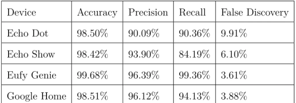
6.2 Baselines

In this section I establish the baseline classification accuracy of the trained models. The purpose of this section is to demonstrate the levels of accuracy that were established by the models without filtering in place or background traffic included.

A detailed description of how the features and models were selected, corresponding confusion matrices as well as further information on the models trained only on certain protocols and services are available in the Appendices.

Device Accuracy Precision Recall False Discovery Echo Dot 98.50% 90.09% 90.36% 9.91%

Echo Show 98.42% 93.90% 84.19% 6.10% Eufy Genie 99.68% 96.39% 99.36% 3.61% Google Home 98.51% 96.12% 94.13% 3.88%

Table 6.4: Baseline Performance of Random Forest classifier Device Accuracy Precision Recall False Discovery Echo Dot 99.83% 97.59% 96.33% 2.41%

Echo Show 99.88% 97.66% 98.41% 2.34% Eufy Genie 99.98% 99.98% 99.96% 0.02% Google Home 99.96% 99.79% 99.83% 0.21%

Table 6.5: Performance of model trained on HTTP(S)

Table 6.5 shows the baseline performance of the Random Forest when trained on HTTP and HTTPS connections only.

6.3 Experiment 1: K-Means Clustering

In this section I present the results obtained by performing K-Means clustering. All 12 features were used including categorical attributes, such as protocol and service, which needed to be transformed to numerical values.

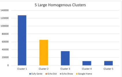
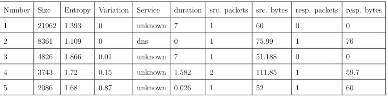
The results achieved in this experiment filter confirmed the claim that devices behavior tended to form either homogenous or heterogenous clusters. In Table 6.6 and Table YY I present some of the larger clusters observed to demonstrate this pattern. These results ultimately served as the rationale for the implementation of a filter which is introduced in the next experiment.

Figure 6.1: 5 Large Homogenous Clusters

Cluster Size Entropy Variation Service duration src. packets src. bytes resp. packets resp. bytes

1 127256 0.0005 0 http 7 5 337 5 933

2 65143 0 0 http 7 6 391 4 299

3 36034 0 0 http 7 5 337 5 636

4 10749 0 0.02 http 7.397 5 336.05 5 589.15

5 11128 0.104 0.17 other 1.949 2 120 0 0

Figure 6.2: 5 Large Heterogenous Clusters

Number Size Entropy Variation Service duration src. packets src. bytes resp. packets resp. bytes

1 21962 1.393 0 unknown 7 1 60 0 0

2 8361 1.109 0 dns 0 1 75.99 1 76

3 4826 1.866 0.01 unknown 7 1 51.188 0 0

4 3743 1.72 0.15 unknown 1.582 2 111.85 1 59.7

5 2086 1.68 0.87 unknown 0.026 1 52 1 60

Table 6.7: 5 Large Heterogenous Clusters

Some key observations from homogenous clusters include:

• The Eufy Genie was the device most commonly found in homogenous clusters. • Amazon devices were less likely to form highly homogenous clusters

• Homogenous clusters tended to contain HTTP and HTTPS traffic • Homogenous clusters typically involved multi-packet exchanges

• Entropy is a sensitive measurement. Even a very small proportion of connections from different devices will lead to significantly higher entropy than a pure cluster. Some key observations from heterogeneous clusters include:

• All four devices appeared in many of the clusters

• Clusters tended to contain DNS or traffic from unknown services • Clusters typically involved short or single-packet exchanges

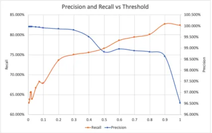
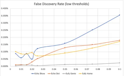
6.4 Experiment 2: Introducing the Filter

Given the results in Experiment 5, implementing the filter appeared to be a viable method of reducing false positives. To derive an appropriate entropy threshold It was necessary to examine the relationship between maximum allowed entropy and model performance. I varied the entropy threshold from 0 to 1 measuring the effect on both precision and recall. Results are only plotted for the lower half of entropy thresholds (less than 1), and as filtering with larger entropy thresholds are not useful given the

goals of this work.

Figure 6.3 shows that as the entropy threshold approaches 0, the Echo Show and Echo Dot have a significant portion of their traffic filtered out, meaning that their connections tended to cluster heterogeneously. On the other hand, the Eufy Genie only has a small amount of traffic filtered out indicating that its connections cluster homogeneously. Therefore, the percentage of connections filtered out at low entropy thresholds can be viewed as a measure of the uniqueness of device behavior.

In Figure 6.4, the amount of traffic remaining for each service is plotted as the entropy threshold decreases. It can be seen that traffic from unknown services are filtered out at a much faster rate while http and https traffic does not decrease significantly.

At this point is important to note that moving forward performance is calculated considering both the filtering and classification portions of the model. In other words, filtered data is taken into account when calculating performance metrics. This means

Figure 6.3: Connections Filtered