How are VIX and Stock Index ETF Related?

ISSN: 2341-2356

WEB DE LA COLECCIÓN: http://www.ucm.es/fundamentos-analisis-economico2/documentos-de-trabajo-del-icaeWorking

Instituto

Complutense

de Análisis

Económico

How are VIX and Stock Index ETF Related?

Chia-Lin Chang

Department of Applied Economics Department of Finance National Chung Hsing University, Taiwan

Tai-Lin Hsieh

Department of Applied Economics National Chung Hsing University

Taichung, Taiwan Michael McAleer

Department of Quantitative Finance National Tsing Hua University, Taiwan and Econometric Institute Erasmus School of Economics Erasmus University Rotterdam and

Tinbergen Institute, The Netherlands and

Department of Quantitative Economics Complutense University of Madrid, Spain

Abstract

As stock market indexes are not tradeable, the importance and trading volume of Exchange Traded Funds (ETFs) cannot be understated. ETFs track and attempt to replicate the performance of a specific index. Numerous studies have demonstrated a strong relationship between the S&P500 Composite Index and the Volatility Index (VIX), but few empirical studies have focused on the relationship between VIX and ETF returns. The purpose of the paper is to investigate whether VIX returns affect ETF returns by using vector autoregressive (VAR) models to determine whether daily VIX returns with different moving average processes affect ETF returns. The ARCH-LM test shows conditional heteroskedasticity in the estimation of ETF returns, so that the diagonal BEKK model is used to accommodate multivariate conditional heteroskedasticity in the VAR estimates of ETF returns. Daily data on ETF returns that follow different stock indexes in the USA and Europe are used in the empirical analysis. The estimates show that daily VIX returns have: (1) significant negative effects on European ETF returns in the short run; (2) stronger significant effects on single market ETF returns than on European ETF returns; and (3) lower impacts on the European ETF returns than on S&P500 returns.

Keywords Stock market indexes, Exchange Traded Funds, Volatility Index (VIX), Vector

autoregressions, moving average processes, conditional heteroskedasticity, diagonal BEKK.

JL Classification C32, C58, G12, G15. UNIVERSIDAD COMPLUTENSE MADRID

Working Paper nº 1602

February, 2016

How are VIX and Stock Index ETF Related?*

Chia-Lin Chang

Department of Applied Economics Department of Finance National Chung Hsing University

Taichung, Taiwan

Tai-Lin Hsieh

Department of Applied Economics National Chung Hsing University

Taichung, Taiwan

Michael McAleer

Department of Quantitative Finance National Tsing Hua University, Taiwan

and

Econometric Institute, Erasmus School of Economics Erasmus University Rotterdam

and

Tinbergen Institute, The Netherlands and

Department of Quantitative Economics Complutense University of Madrid, Spain

Revised: February 2016

* For financial support, the first author wishes to thank the National Science Council, Taiwan, and the third author is grateful to the National Science Council, Taiwan and the Australian Research Council.

Abstract

As stock market indexes are not tradeable, the importance and trading volume of Exchange Traded Funds (ETFs) cannot be understated. ETFs track and attempt to replicate the performance of a specific index. Numerous studies have demonstrated a strong relationship between the S&P500 Composite Index and the Volatility Index (VIX), but few empirical studies have focused on the relationship between VIX and ETF returns. The purpose of the paper is to investigate whether VIX returns affect ETF returns by using vector autoregressive (VAR) models to determine whether daily VIX returns with different moving average processes affect ETF returns. The ARCH-LM test shows conditional heteroskedasticity in the estimation of ETF returns, so that the diagonal BEKK model is used to accommodate multivariate conditional heteroskedasticity in the VAR estimates of ETF returns. Daily data on ETF returns that follow different stock indexes in the USA and Europe are used in the empirical analysis. The estimates show that daily VIX returns have: (1) significant negative effects on European ETF returns in the short run; (2) stronger significant effects on single market ETF returns than on European ETF returns; and (3) lower impacts on the European ETF returns than on S&P500 returns.

Keywords: Stock market indexes, Exchange Traded Funds, Volatility Index (VIX), Vector autoregressions, moving average processes, conditional heteroskedasticity, diagonal BEKK.

1. Introduction

One of the major reasons why great importance is attached to risk management in financial markets is that the vigorous growth of derivative financial products has resulted in increased market risk and uncertainty. As risk is a latent variable, its measurement is an important issue. How to search for the minimum amount of risk based on a specific return on assets, or to pursue the maximum returns based on a given level of risk, is an issue that has long concerned institutional and individual investors in finance and economics, among other areas.

There are many different categories of risk. The risk associated with the returns on future investments is referred to as investment risk which, together with the rise in the associated hedging theory, indicates that market participants are becoming increasingly interested in understanding the information implied in market changes. Regardless of whether risk management relies on the volatility index (VIX), compiled by the Chicago Board Options Exchange (CBOE), or the autoregressive conditional heteroskedasticity (ARCH) proposed by Engle (1982), who is credited with initiating the dynamic analysis of financial volatility, such analysis is intended to provide a correct and accurate method of estimating risk to lead to effective and optimal risk management and sensible dynamic hedging strategies..

When market participants are interested in analyzing the extent of future fluctuations in the stock market via the options market to achieve their objective of hedging risk, they will take numerous factors into consideration, such as different maturity dates, the exercise prices of the option prices, among others. However, the comprehensive analysis performed by potential investors in relation to the information on the

different factors is time consuming and arduous. The volatility index (VIX) that is compiled by the CBOE greatly reduces some of the difficulties expected by investors in terms of the expected volatility of the index.

Put simply, VIX is based on using all of the closest at-the-money call and put S&P500 index option premium prices in the most recent month and the second month to obtain indirectly the weighted average of the implied volatility series. Prior to 2003, the method used to calculate VIX involved selecting a total of 8 series for the closest at-the-money call and put S&P100 index options for the most recent month and the second month, and obtaining the weighted average of the index after calculating the implied volatility.

The implied volatility mainly reflects the average expectations of market investors in regard to the volatility of the S&P 500 index over the next 30 days. For this reason, the size of VIX captures how much the investor is willing to pay to deal with their own investment risk. The larger is the index, the more pronounced are the expectations regarding the future volatility in the index, meaning that the investor feels unsure about market conditions. The smaller is the index, the greater is the tendency for the changes in the stock market index to diminish, and hence for the index to fall within a narrower range.

Therefore, VIX can be seen as representing the level of fear expected by many investors in the market, or the “investor fear gauge”. As an example, when the stock market continues to exhibit a downward trend, VIX will continue to rise, and when the VIX appears to be unusually high or low, this means that investors who become panic-stricken may not count the cost of the put option, or may be excessively

optimistic without engaging in any hedging action.

Figure 1 depicts the trends in the S&P 500 index and VIX for 1990 to 2014, and indicates that the highest point for VIX rises sharply from the beginning of September 2008 to its highest historical level in November 2008, when it reached a record high point (80.86). Asymmetrical characteristics of VIX can also be observed. When the global financial crisis occurred in 2008-2009, the trend of VIX immediately reflected the panic on the part of market participants. As VIX was at a very high level, this might have indicated that the market would rebound, and that the stock price index would increase. History records that this did not happen quickly.

Previous studies have shown that the highly volatile market environment when VIX is at a peak can help predict future rises in the stock market index. When the market is highly volatile, the stock index falls along with the increase in VIX by more than the market, which is characterized by low volatility. This indicates that when the market is characterized by a highly volatile environment, the negative impact of VIX is relatively more severe (Giot, 2005; Sarwar, 2012).

[Insert Figure 1here]

From Figure 1, we can see a very interesting phenomenon, namely when VIX rises rapidly, the S&P 500 index tends to fall simultaneously, which usually means that the index is not far from its lowest level. On the contrary, when VIX has already fallen to its lowest point and starts to rise again, and the stock market index is in a bullish phase, this means that the time for the market index to rebound is gradually approaching. Although trends in the stock market index do not always follow a certain

course, and the prices and returns of financial derivatives such as futures and options are affected by current news and other technical indicators, the probability of investors predicting future trends in the index can be improved greatly by using VIX, so that risk management strategies are likely to be enhanced.

There have been numerous studies in the past on the VIX and market index returns for the market as a whole, with the focus of the research being mostly on the broader market index returns and on discussing the ability of VIX to forecast option prices. As described above, VIX is an important market risk indicator that is used to predict future index volatility, especially in interactive global markets with their diversified portfolios, where investors cannot rule out the risk of changes in the US stock market that might cause fluctuations in the stock markets of other countries. Using stock market returns data for the BRIC (Brazil, Russia, India and China) countries, Sarwar (2012) found that VIX not only influenced US stock market index returns, but that it also had a significant influence on the BRIC market indexes.

In recent years, there has been a vigorous expansion of a wide range of financial market indexes that have provided investors with information to understand the index of crude oil and other energy issues, gold-related indexes, bond-related indexes or index strategies, social enterprise indexes, high dividend yield indexes, low volatility indexes, as well as a wide range of sub-indexes for various industries,. In fact, there have been so many indexes that recording them comprehensively would be difficult. However, while the indexes measure the performance of the market and economic growth, in the absence of trading on spot indexes, this has resulted in the generation of exchange traded funds and many other financial derivatives (for a recent critical econometric analysis of financial derivatives, see Chang and McAleer, 2015).

The ETF (exchange traded fund) uses the “index” as a benchmark, selecting the constituent parts of the index as investment targets, in order to achieve the objective of replicating the broader market index performance. Although the ETF is referred to as a fund, it is different from what the general investing public refers to as a fund. The term “fund” usually refers to an open-end mutual fund, and is different in nature from an ETF. A mutual fund is part of an actively managed investment portfolio, but an ETF is a passively managed fund.

Furthermore, if the investor wants to buy or sell a mutual fund, it can only be redeemed with the asset management company that issued the mutual fund, according to the net worth of the fund at the close of the day on which it was traded. As for the way in which the ETF is traded, this is relatively simple in that the ETF is traded at the listed price, and can be traded directly with other investors using the market price.

As the ETF replicates the performance of the broader market index, unless there is a change in the constituent parts of the index that is tracked, fund managers will not access the market frequently, so there will typically be few changes made to the ETF portfolios. The securities brokerage fees that need to be paid for funds will thereby be reduced significantly compared with actively managed funds, and will become another feature of passively managed funds that attracts investors.

In reviewing the performance of all funds in the market, it has been found that the returns on mutual funds are frequently lower than the average returns for the market as a whole. It is seldom the case that mutual funds can continue to beat the market and remain sufficiently stable to earn excess profits. In other words, when compared with

market funds for which the stocks are selected based on active strategies, ETFs that track the market index are more profitable. If their low management fees are also taken into consideration, the greater will be the gap between the two in terms of their relative profitability.

Europe is an important economic and financial region, and a single country’s market index reflects that region’s economic performance, such as the Financial Times Stock Exchange index, or FTSE100, which consists of 100 stocks that are traded on the London Stock Exchange. The 100 stocks are mostly those of major British companies, but also include a small number of companies from nine other European countries.

The CAC40 index has since 1988 been made up of the 40 largest listed companies’ stocks that are traded on the Paris Bourse. The DAX index is made up of 30 selected blue-chip companies whose shares are traded on the Frankfurt Stock Exchange in Germany. Besides being calculated on the basis of market value, the DAX index is also determined by attaching weights to the 30 stocks being compiled based on expected dividend considerations. The FTSE100, CAC40 and DAX, respectively, are the indexes of economic performance that reflect the three major European capital markets of the UK, France and Germany, and have an important role to play in enabling investors to understand the dynamics of the European economy.

Unlike single-country stock indexes that only consist of the stocks listed on those individual countries’ stock exchanges, the regional indexes to which relatively large numbers of market participants currently pay attention are the MSCI Europe Index, EURO STOXX50 index, MSCI Europe Union Index, among others. The compilation of regional indexes is arbitrary, so that it is necessary to examine the approach used by

the index issuing companies. For example, the EURO STOXX50 index selects only

50 weighted stocks from among all European industries, while the MSCI Europe Index consists of 500 stocks.

Although selecting a larger number of stocks means that the respective index will embody the characteristics of the industries in the region, this will dilute the impact of the industry leading shares on the overall index. Therefore, the kind of index that best represents the economic performance in Europe will be decided by the market participants. Moreover, the MSCI series of European regional indexes consists of almost 10 different kinds of indexes, the differences between them being small, which can easily cause confusion. Thus, when investors refer to European stock markets, they will usually first observe the EURO STOXX50 index, and thereby examine the overall performance of the European stock markets.

The EURO STOXX50 index is comprised of 50 blue-chip stocks from various industries within the European area, with 12 European countries being covered by the stocks. Derivative financial products related to the EURO STOXX50 index include futures, options and ETFs that track the EURO STOXX50 index. The EURO STOXX50 index and the ETF can depict the overall trend of the European market, and reflects European corporate earnings prospects and market conditions.

The objective of the ETF is to expect to earn the same return as the market index, but investors must still decide when to buy and sell the ETF in order to realize a gain or a loss. When implementing a trading strategy, if institutional or individual investors can fully understand the market index being tracked by the ETF, it may then be possible to reduce the investment risk.

Although the ETF is a derivative financial commodity that has become widely available within the last decade, previous research does not seem to have performed any serious statistical analysis of ETF returns with VIX. Therefore, a primary purpose of the paper is to investigate the extent to which US stock market risk indicators affect European markets, and to compare the similarities and differences between an ETF issued by a single country and the market index of the country, as well as an ETF for the European area that is influenced by VIX.

In order to reduce any possible biases in the calculation of the standard errors, the paper uses the Diagonal BEKK multivariate conditional volatility model to adjust for the residual multivariate conditional heteroskedasticity so that a robust comparison of the empirical results can be drawn before and after such corrections have been made.

The remainder of the paper proceeds as follows. The literature on VIX is reviewed in Section 2. In Section 3, we present the VAR and Diagonal BEKK models. A description of the sample and variables follows in Section 4. This is followed by the empirical results in Section 5, and some concluding remarks are given in Section 6.

2. VIX Literature Review

With regard to the extant research on the relationship between VIX and US stock market returns, Sarwar (2012) uses US stock market data for the period 1993-2007, and finds that VIX and US stock market returns are negatively correlated over the period. Moreover, the negative relationship is especially significant when the US stock market is characterized by a high degree of volatility. Sarwar (2012) also

examines the impact of VIX on the market returns of the four BRIC countries, and finds that a significant negative relationship exists between VIX and the Chinese and Brazilian stock markets, and that the negative relationship is particularly strong when the Brazilian stock market is experiencing a high degree of volatility. However, there was apparently no negative relationship between VIX and the Russian and Indian stock markets.

These empirical results suggest strongly that the relationship between stock market returns and VIX is asymmetric (also see Giot, 2005). This paper confirms that VIX is not only applicable to the US stock market, but that it can also be used to explain movements in stock markets in other countries. Previous studies have also used VIX to capture the impact of investor sentiment on stock returns. By separating market participants into institutional investors and individual investors, several studies have found that institutional investors tend to be more easily impacted by macroeconomic variables, financial ratios and other related variables, and that VIX has a smaller impact on stock returns than the macroeconomic variables and financial ratios (see, among others, Arik, 2011; Fernandes et al., 2014).

In addition to the relationship between VIX and US stock market returns, Cochran et al. (2015) use fuel oil, gasoline and natural gas futures prices returns data for the period 1999-2013, and find that natural gas futures returns and changes in VIX are positively correlated. However, changes in VIX are negatively correlated for heating oil and gasoline, thereby suggesting that the returns on natural gas, contrary to the returns on the other two commodities, are more able to withstand the volatility or risk in the stock market.

This phenomenon is particularly significant during the global financial crisis of 2008-2009. This paper confirms empirically that the impact of the returns of VIX is not limited to the stock market index returns, but that the index also exerts considerable influence on the spot and futures price returns for the three energy commodities in heating oil, gasoline and natural gas.

There are currently many methods that are used to measure volatility, such as the historical variance or standard deviation of observed returns. Such methods are exceedingly simple and static, meaning the risk measure does not incorporate any shocks that might change over time, so it is natural that there are inherent shortcomings. For example, the volatility of the returns on risky assets may be characterized by fat-tail distributions, asymmetry, clustering, persistence, or mean

reversion(see, for example, Poon and Granger, 2003).

For this reason, there are many methods used to measure risk in empirical research, such as historical volatility, implied volatility, expected volatility, VIX, conditional volatility, stochastic volatility, and realized volatility. The volatility measure that is the easiest to understand is historical volatility, which uses data on events that have already taken place to calculate volatility, and is therefore regarded as a backward-looking index.

The other two indexes that are based on conditional and implied volatility may be explained in a straightforward manner, as follows:

(1) Conditional volatility: As the unconditional and conditional variances of asset returns are assumed to be constant, this approach was unable to reflect the fact that the

conditional variance actually changes dramatically over time when high frequency data are used. Engle (1982) proposed an autoregressive conditional heteroskedasticity (ARCH) model which incorporated the heterogeneity of the conditional variance and volatility clustering of the time series variables to bring the model closer to reality. Bollerslev (1986) extended the ARCH model by proposing a generalized autoregressive conditional heteroskedasticity (GARCH) model to broaden the model’s applicability.

The GARCH model includes two effects, namely the ARCH effect that captures the short-term persistence of returns shocks on conditional volatility, and the GARCH effect that contributes to the long-term persistence of returns shocks on conditional volaitlity. Tsay (1987) showed that the ARCH model could be derived from a random coefficient autoregressive process.

As the GARCH model is unable to capture the asymmetric effects of positive and negative shocks of equal magnitude on the subsequent conditional volatility, Glosten et al. (1993) modified GARCH to the GJR model by including an indicator variable to distinguish between positive and negative shocks. Numerous studies have found that the GJR model has useful explanatory power in distinguishing between positive and negative shocks on the conditional volatility of daily stock returns (see, among others, Ling and McAleer, 2003).

In addition, Nelson (1991) proposed the exponential GARCH, or EGARCH, model. Besides capturing the asymmetric effect of the unexpected impact on the conditional variance, this model purports to capture the important leverage effect of shocks on the volatility of financial assets, based on the debt-equity ratio. Leverage refers to the

outcome in which the effects of negative returns shocks on volatility are greater than those of positive shocks of equal magnitude.

McAleer (2005, 2014) analysed GARCH and alternative conditional volatility models that incorporate asymmetry, but not leverage, which was shown to be excluded from derivations that are based on the random coefficient autoregressive approach. For a detailed derivation and the statistical properties of the EGARCH model, see McAleer and Hafner (2014).

From a practical perspective, Kanas (2013) used the GARCH model to engage in

out-of-sample forecasting in relation to the excess returns data for the S&P500 index for 1990-20061 The empirical results indicated that the explanatory power of the GARCH model with VIX was better than that of the GARCH model without VIX, or where VIX was used on its own.

Following the establishment of financial asset diversification and investment portfolios, several different multivariate conditional volatility models have been derived, such as the constant conditional correlation (CCC) model (Bollerslev, 1990), dynamic conditional correlation model (Engle, 2002), varying conditional correlation model (Tse and Tsui, 2002), VARMA-GARCH model (Ling and McAleer, 2003), and VARMA-AGARCH model (McAleer et al., 2009).

(2) Implied volatility: As volatility is a latent variable, the concept of implied volatility involves incorporating the specific strike price and the option price on the maturity date into an option pricing formula to infer indirectly or imply the volatility

1

Using the S&P 500 index excess returns obtained after subtracting adjusted dividends from one-month Treasury bills.

of the option. In order to derive the implied volatility, it is necessary to use an appropriate option pricing model.

While the well-known Black-Scholes option pricing model is widely used, the shortcoming of this model is that it assumes that the variance of the stock price returns is fixed, which does not accord with what is actually observed in markets, namely: (1) different levels of implied volatility are inherent in the strike price, and (2) implied volatility in-the-money and out-of-the-money is greater than the implied volatility at-the-money (also known as the implied volatility smile). In view of this drawback, different evaluation models have been proposed, such as a binomial tree model to evaluate the proposed option price (see Cox et al., 1979; Dumas et al., 1998; Rosenberg, 1999; Borovkova and Permana, 2009).

Another kind of implied or expected volatility measure is the VIX volatility index, which was used by the CBOE in 1993 to serve as a market volatility thermometer. Prior to 2003, VIX was calculated by selecting S&P 100 index options based on the call and put options closest to the price level for the most recent month and the second month for a total of eight series. This involved reweighting the average of the indexes obtained after calculating their implied volatility.

As the trading volume of S&P 500 index options gradually increased, in 2003 the CBOE started to calculate VIX based on S&P 500 index option prices. The CBOE retained, and continued to calculate and announce, the original volatility index based on the S&P 100 index option prices, but changed the acronym to VXO.

S&P500 index option premium prices in the most recent month and the second month to obtain indirectly the weighted average of the volatility series. VIX is, in effect, an expected volatility series, with the integration process being model free. In early 2001, the COBE announced VXN, which uses the same method as for calculating VIX, but is based on the NASDAQ100 index options prices.

Previous studies have suggested that, although VIX is not necessarily able to predict accurately the variability in returns, the information it provides serves as a valuable reference to investors, and so it that cannot be ignored when examining the risk-return relationship. As Cochran et al. (2014) noted in their empirical paper, the impact of VIX can be felt not only in the stock market, but also in the returns in the spot commodity and futures markets.

Furthermore, in previous empirical research on the correlation between VIX and market weighted index returns, the focus of attention has been mostly on the market weighted index returns and on investigating the ability of VIX as a proxy variable for volatility to forecast option prices. To the best of our knowledge, there has been little or no research on the relationship between VIX and ETF returns for market indexes outside the USA. This is an omission exclusion that should be remedied as VIX not only influences the US stock market, but almost certainly affects the stock market returns of other countries.

The ETF is a derivative financial product that has come to prominence during the last decade, and the volatility of returns on risk-based assets has increasingly drawn the attention of institutional and individual investors. How to use the information provided by the volatility of ETF to enable investors to achieve optimal risk

management is of serious concern from a practical perspective. Therefore, this paper will examine the impact of US financial markets on European financial markets, and also assess the extent to which ETF returns based on European market indexes have been influenced by the US VIX.

3. VAR and Diagonal BEKK Models

3.1 VAR(p)

VAR is an n-equation linear model in which each variable is explained by its own lagged values, together with the previous values of the other n-1 variables. Consider a vector autoregressive model of a set of M endogenous variables, as follows:

𝒀𝒀𝒕𝒕 = 𝑪𝑪+𝑨𝑨𝟏𝟏𝒀𝒀t−1+⋯+𝑨𝑨𝒑𝒑𝒀𝒀t−p+𝜺𝜺𝐭𝐭 (1)

where 𝒀𝒀_𝒕𝒕 and 𝜺𝜺_𝐭𝐭 are each 𝑀𝑀× 1 vectors of random variables,

𝒀𝒀𝒕𝒕 = (𝑦𝑦1𝑡𝑡,𝑦𝑦2𝑡𝑡, … . ,𝑦𝑦𝑚𝑚𝑡𝑡) for = 1,2, … .𝑀𝑀, and 𝜺𝜺𝐭𝐭 = (𝜀𝜀1t,𝜀𝜀2t, … . ,𝜀𝜀mt). 𝑪𝑪 is the

mean vector, and 𝑨𝑨_𝟏𝟏, … ,𝑨𝑨_𝒑𝒑, and 𝛀𝛀= [𝒗𝒗_𝒕𝒕𝒗𝒗_𝒕𝒕′] are 𝑀𝑀×𝑀𝑀 parameter matrices. In the paper, we use VAR(1) for the three series, 𝑦𝑦_1𝑡𝑡, 𝑦𝑦_2𝑡𝑡, 𝑦𝑦_3𝑡𝑡 . The vector autoregressive process is given as follows:

�𝑦𝑦𝑦𝑦1𝑡𝑡2𝑡𝑡 𝑦𝑦3𝑡𝑡 �=�𝑐𝑐𝑐𝑐12 𝑐𝑐3 �+�𝑎𝑎𝑎𝑎1121 𝑎𝑎𝑎𝑎1222 𝑎𝑎𝑎𝑎1323 𝑎𝑎31 𝑎𝑎32 𝑎𝑎33 � �𝑦𝑦𝑦𝑦1𝑡𝑡−12𝑡𝑡−1 𝑦𝑦3𝑡𝑡−1 �+�𝜀𝜀𝜀𝜀1𝑡𝑡2𝑡𝑡 𝜀𝜀3𝑡𝑡 � (2)

where each equation contains an error that has zero expectation, given the previous information on 𝑦𝑦_1𝑡𝑡, 𝑦𝑦_2𝑡𝑡, 𝑦𝑦_3𝑡𝑡.

An autoregressive process describes the dynamic behaviour among the endogenous and exogenous variables in the system. It is possible to add other lagged exogenous variables, such as 𝑤𝑤_𝑡𝑡−1, to equation (1), which leads to equation (2):

�𝑦𝑦𝑦𝑦1𝑡𝑡2𝑡𝑡 𝑦𝑦3𝑡𝑡 �= �𝑐𝑐𝑐𝑐12 𝑐𝑐3 �+�𝑎𝑎𝑎𝑎1121 𝑎𝑎𝑎𝑎1222 𝑎𝑎𝑎𝑎1323 𝑎𝑎31 𝑎𝑎32 𝑎𝑎33 � �𝑦𝑦𝑦𝑦1𝑡𝑡−12𝑡𝑡−1 𝑦𝑦3𝑡𝑡−1 � + [𝑏𝑏1 𝑏𝑏2 𝑏𝑏3]� 𝑤𝑤𝑡𝑡−1 𝑤𝑤𝑡𝑡−1 𝑤𝑤𝑡𝑡−1 �+�𝜀𝜀𝜀𝜀1𝑡𝑡2𝑡𝑡 𝜀𝜀3𝑡𝑡 � (3)

where equation (3) can be estimated efficiently by ordinary least squares (OLS), depending on the cross-equation restrictions and the structure of the system covariance matrix. We also test if the returns shocks has conditional heteroskedasticity by using the multivariate ARCH-LM tests (see, among others, Engle, 1982; Hamilton, 1994; Lütkepohl, 2006).

The multivariate ARCH-LM test is based on the following regression:

𝑣𝑣𝑣𝑣𝑐𝑐ℎ�𝜺𝜺�𝐭𝐭𝜺𝜺�𝐭𝐭′�= 𝜷𝜷𝟎𝟎+𝑩𝑩𝟏𝟏𝑣𝑣𝑣𝑣𝑐𝑐ℎ�𝜺𝜺�𝐭𝐭−𝟏𝟏𝜺𝜺�𝐭𝐭−𝟏𝟏′�+⋯+𝑩𝑩𝒒𝒒𝑣𝑣𝑣𝑣𝑐𝑐ℎ�𝜺𝜺�𝐭𝐭−𝐪𝐪𝜺𝜺�𝐭𝐭−𝐪𝐪′�+𝒗𝒗𝒕𝒕 (4)

where 𝒗𝒗_𝒕𝒕 is a spherical error process, and vech is the column-stacking operator for symmetric matrices that stacks the columns from the main diagonal upward or downward, but not both, owing to symmetry. The dimension of 𝜷𝜷_𝟎𝟎 is 1

2𝑀𝑀(𝑀𝑀+ 1)

and, for coefficient matrices, 𝑩𝑩_𝟏𝟏, i = 1,2,…, q, has covariance matrix dimension

given by 1

2𝑀𝑀(𝑀𝑀+ 1) × 1

2𝑀𝑀(𝑀𝑀+ 1). The mull hypothesis is 𝐻𝐻0:𝑩𝑩1 =𝑩𝑩2 = ⋯=

𝑩𝑩𝑞𝑞 = 0, for which the test statistic is given as:

VARCH𝐿𝐿𝐿𝐿(𝑞𝑞) =1₂𝑇𝑇𝑀𝑀(𝑀𝑀+ 1)𝑅𝑅𝑚𝑚2

𝑅𝑅𝑚𝑚2 = 1−_{𝑀𝑀(𝑀𝑀}2_{+ 1)}𝑡𝑡𝑡𝑡(Ω�Ω�−1)

where Ω� is the covariance matrix of the regression model in equation (1). The test statistic is distributed under the null hypothesis as χ2(𝑞𝑞𝑀𝑀2(𝑀𝑀+ 1)2⁄4). In this paper, we use a VAR(1) model with 3 endogenous variables, so that the test statistic is distributed as 𝑇𝑇×𝑅𝑅2~𝜒𝜒2(36).

3.2. Diagonal BEKK

As shown in Chang, Yi, and McAleer (2015), among others, the multivariate extension of univariate GARCH is presented in Baba et al. (1985) and Engle and Kroner (1995). Consider a VAR(1) model, and recall the equation (1) is given as:

𝒀𝒀𝒕𝒕 =𝐸𝐸(𝒀𝒀𝒕𝒕|𝐼𝐼𝑡𝑡−1) +𝜺𝜺𝒕𝒕 (5)

The multivariate definition of the relationship between 𝜺𝜺_𝒕𝒕 and 𝜼𝜼_𝒕𝒕 is given as:

where 𝑫𝑫_𝒕𝒕 = 𝑑𝑑𝑑𝑑𝑎𝑎𝑑𝑑(ℎ_1𝑡𝑡,ℎ_2𝑡𝑡, … ,ℎ_{𝑚𝑚𝑡𝑡}) is a diagonal matrix comprising the univariate conditional volatilities. As shown in Chang, Yi, and McAleer (2015), in order to establish volatility spillovers in a multivariate framework, it is useful to define the multivariate extension of the relationship between the returns shocks and the standardized residuals, that is, 𝜼𝜼_𝒕𝒕 = 𝜺𝜺_𝒕𝒕⁄�ℎ_𝑡𝑡 , as 𝜼𝜼_𝒕𝒕 is an 𝑚𝑚× 1 vector that is assumed to be iid for all m elements.

Define the conditional covariance matrix of 𝜀𝜀_𝑡𝑡 as 𝑸𝑸_𝒕𝒕:

where 𝚪𝚪_𝒕𝒕 is theconditional correlation matrix of 𝜼𝜼_𝒕𝒕.

In order to lead to the diagonal BEKK model, as shown in McAleer et al. (2008) and Chang, Yi, and McAleer (2015), the vector random coefficient autoregressive process of order one is given as:

(8)

where 𝜀𝜀_𝑡𝑡and 𝜂𝜂_𝑡𝑡 are 𝑚𝑚× 1 vectors, and Φ_t is an 𝑚𝑚×𝑚𝑚 matrix of random coefficients, with Φ_𝑡𝑡~𝑑𝑑𝑑𝑑𝑑𝑑(0,𝐴𝐴) and 𝜂𝜂_𝑡𝑡~𝑑𝑑𝑑𝑑𝑑𝑑(0,𝑄𝑄𝑄𝑄′).

Technically, a vectorization of either a full or Hadamard matrix A, neither of which is diagonal, to vec 𝐴𝐴, without symmetry, can have dimension as high as m2×m2 , whereas vectorization of a symmetric matrix A to vech 𝐴𝐴 can have dimension as low as m(m−1)/2×m(m−1)/2 (for further details, see McAleer et al., 2008; Caporin and McAleer, 2012, 2013 ).

If 𝐴𝐴 is either a diagonal matrix or the special case of a scalar matrix, 𝐴𝐴= 𝑎𝑎𝐼𝐼_𝑚𝑚, McAleer et al. (2008) showed that the multivariate extension of GARCH(1,1) from equation (8), incorporating an infinite geometric lag in terms of the returns shocks, is given as the diagonal or scalar BEKK model, namely:

𝑄𝑄𝑡𝑡 =𝑄𝑄𝑄𝑄′+𝐴𝐴𝜀𝜀𝑡𝑡−1𝜀𝜀𝑡𝑡−1′𝐴𝐴′+𝐵𝐵𝑄𝑄𝑡𝑡−1𝐵𝐵′ (9)

where A and B are both either diagonal or scalar matrices, namely:

𝐀𝐀= diag(𝑎𝑎)；_{𝐁𝐁= diag(𝑏𝑏}) 𝐀𝐀=�𝑎𝑎11⋮ ⋯⋱ 0⋮ 0 ⋯ 𝑎𝑎𝑚𝑚𝑚𝑚 �，𝐁𝐁= �𝑏𝑏11⋮ ⋯⋱ 0⋮ 0 ⋯ 𝑏𝑏𝑚𝑚𝑚𝑚 �，𝐂𝐂= � 𝑐𝑐11 ⋯ 𝑐𝑐1𝑚𝑚 ⋮ ⋱ ⋮ 0 ⋯ 𝑐𝑐𝑚𝑚𝑚𝑚 �。

The diagonal BEKK model is given as:

𝑄𝑄𝑡𝑡 =𝑄𝑄𝑄𝑄′+ diag(𝑎𝑎)𝜀𝜀𝑡𝑡−1𝜀𝜀𝑡𝑡−1′ diag(𝑎𝑎) + diag(𝑏𝑏)𝑄𝑄𝑡𝑡−1diag(𝑏𝑏) = Q′_{Q + (𝑎𝑎𝑎𝑎}′_{)∘ ε}

t−1ε′t−1+ (𝑏𝑏𝑏𝑏′)∘Ht−1

McAleer et al. (2008) proved that the Quasi-Maximum Likelihood Estimators (QMLE) of the parameters of the diagonal or scalar BEKK models were consistent and asymptotically normal, so that standard statistical inference for testing hypotheses is valid.

4. Data and Variables

In order to comply with the pursuit of index-based investment and the spirit of similar returns for the overall market index, this paper selects ETFs that track three major US stock market indexes, namely SPY, DIA and ONEQ, as well as the ETFs for three major European stock market indexes, namely FEZ, DBXD and XUKX. The daily closing prices for each of the ETF variables are sourced from Yahoo Finance, while the VIX data are sourced from the official CBOE website.

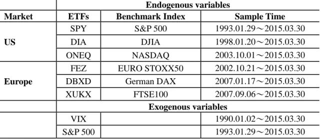
Table 1 illustrates the indexes tracked by each ETF and the sample periods. The endogenous variables used in the paper include the ETF daily return rate. The rate of return is obtained as the logarithm difference of the daily closing price data, multiplied by 100, and will be referred to as the R_variable.

In what follows, we will briefly introduce each ETF and the underlying index that it is tracking. As for the various indexes existing in the actual market, the method used to compile each index is based on the discretion of the index issuing company, with the information conveyed by, and the meaning of each index being based on, the judgement of the index user.

SPY refers to the SPDR S&P 500 ETF. It is worth noting that SPY was the world’s first ETF, and was listed on the New York Stock Exchange in 1993. In addition, as SPY was listed a long time before the other ETFs came on to the market, the fund’s accumulated net worth is the ETF market’s largest. SPY tracks the S&P 500 composite index, and is the fund that is the most able to represent the US stock market’s performance through the index. The stocks that make up the index are selected from the largest 500 companies in terms of market value listed and traded on the New York Stock Exchange and Nasdaq, and include Microsoft, Apple, P&G, Johnson & Johnson, Morgan Chase, IBM, Coca-Cola, AT&T and other leading companies. The SPY portfolio is made up from the stocks of these 500 companies.

DIA is the SPDR Dow Jones Industrial Average ETF, which tracks the Dow Jones Industrial Average (DJIA). The index is made up of 30 blue chip stocks. Although it is referred to as an industrial index, the proportion allocated to the industrial sector falls

far short of that at the end of the 19th Century, when the index had only just been established, and the index also reflects the core of the transformation of the US economic structure. The calculation of the DIA index is characterized by the compilation of an average index, which differs from the typical indexes that are weighted based on market capitalized value, in that the DJIA is weighted according to price.

The highly-priced stocks making up the index which fluctuate less than the low-priced stocks have more of an impact on the overall DIA index. The DIA portfolio is also limited to the index of these 30 stocks. According to data at the close of trading on 22 May 2015, the closing data show that the top three industrial sectors in the DIA portfolio, ranked by the weight attached to them, were industry 19.78%, the IT industry 17.71%, and the financial sector 16.76%, respectively. The DIA portfolio differed only slightly from the DJIA Average index that it tracked.

ONEQ is the Fidelity Nasdaq Composite Index Tracking Stock Fund, tracks the Nasdaq Composite Index. This comprises more than 5,000 enterprises that are traded on Nasdaq, and is calculated using the weighted market value. Since the ONEQ stock portfolio can involve the selection of more than 5,000 companies, and is much larger than the other ETFs that track the S&P 500 index or the DJIA index ETFs, its portfolio does not replicate that of the Nasdaq composite index. Instead, ONEQ is primarily comprised of large listed stocks that replicate the market value, with the remaining part being selected using the sampling method.

Data compiled after the close of trade on 22 May 2015 show that the fund is made up of stocks for the IT industry accounting for 46.17%, non-essential consumer goods

accounting for 17.57 percent, and the health care industry accounting for 16.92 percent. As in the case of the Nasdaq composite index, the focus of attention is on the performance of high-tech related industries.

This paper selects three ETFs that track three major US stock market indexes, the intention being to examine their performance in terms of tracking each US market index. However, there are still some differences between the three major market indexes in terms of the economic conditions brought about by the US market. Investors generally believe that the S&P 500 index is most able to represent the overall economic performance of the US capital market because, when compared with the industries that comprise the DJIA index the S&P 500 index is relatively broad. Although the NASDAQ100 Composite Index is comprised of many more stocks than the other two, as too great an emphasis is placed on high-tech industry stocks, investors see the Nasdaq Composite index as reflecting the performance of innovative technology and high-tech industries.

This paper selects three ETFs that track the three major European stock market indexes, namely FEZ, DBXD and XUKX, of which the FEZ tracks the EURO STOXX50, which is an index for the European area measuring the performance of European industries. This is unlike the DBXD and XUKX, which track indexes for single countries.

FEZ is the SPDR EURO STOXX 50 ETF, which is the same as the EURO STOXX50 Index in terms of portfolio selection. The underlying index consists of a total of 50 blue chip stocks spread over 12 European countries. According to data after the close of trade on 27 May 2015, the top three industrial sectors comprising the FEZ

constituents were the financial sector accounting for 26.53%, non-essential consumer goods accounting for 11.33%, and industry accounting for 11.03%. There was only a very slight difference between the FEZ index and the underlying EURO STOXX50 which it tracked.

DBXD ETF is db x-trackers DAX® UCITS ETF, the index that it tracks being the German DAX index. This index is used to measure the performance of the German stock market, and is comprised of the 30 German blue chip stocks that are traded on the Frankfurt Stock Exchange. In addition to using the weighted market value, consideration is given to the stock index’s constituent parts to determine the expected dividend. The DBXD portfolio, which consists of the 30 blue chip stocks, is traded in the Euro currency. From the time the DBXD was listed in 2007 to the first quarter of 2015, the rate of return has been 71.68%. The difference between the rates of return for DBXD and the German DAX index over the same period are quite small.

XUKX is the db x-trackers FTSE 100 UCITS ETF, which is the index that tracks FTSE 100, comprises the 100 leading large stocks in terms of market value that are traded on the London Stock Exchange. Although the FTSE 100 index is used to measure the performance of the UK stock market, as the London Stock Exchange is Europe’s financial center, there is no shortage of companies from other European countries whose stocks are listed and traded in London. XUKX has similar characteristics to the FTSE 100 Index in terms of the stocks that comprise its portfolio, with Royal Dutch Shell of the Netherlands, for example, accounting for a 4.62% share of the overall XUKX portfolio.

According to Fernandes et al. (2014), VIX is characterized by a long-term dependency, so this paper uses 10-day and 20-day moving averages for VIX returns, R_VIX, denoted as R10_VIX and R20_VIX, respectively, in an attempt to understand whether the average VIX for different time periods, such as during the previous 10 and 20 days, affects ETF rates of return.

As far as investors in the European markets are concerned, the S&P 500 index best represents the performance of the US stock market. For this reason, the return on the S&P 500 index, with returns given as R_SP500, is regarded as another exogenous variable. For this reason, the 10- and 20-day moving averages, R10_SP500 and R20_SP500, respectively, are used to examine whether the S&P 500 index rate of return for different periods has an impact on the ETF rate of return. From the range of the coordinates on the vertical axes in Figure 2, we can see that using moving averages reduces the extent of the variation in the series. From Figure 3, we can see that VIX exhibits a negative relationship with both the ETF for the US market and the ETFs for the European markets.

[Insert Figures 2 and 3here]

Table 2 presents the descriptive statistics for the variables. It can be seen that the ETF which tracks the index has many values of variables that are very close to, but not the same, as those of the respective index. This arises is because a certain percentage of the financial products of the asset management company that issues the ETF to follow the underlying index are the same as those that make up the market index. It is standard for 80% of such stocks to be the same, though the actual proportion depends on what is disclosed in the ETF prospectus. The asset management company issuing

the ETF also retains the right, based on the principle of passively managing the ETF, to manage independently any excess amounts.

If the skewness coefficient is positive, indicating that this variable is distributed as a right-tailed distribution, most of the observations in the sample are lower than the average of the sample values. On the contrary, if the skewness coefficient is negative, this variable is distributed as a left-tailed distribution, and most of the observations in the sample are greater than the average. If the coefficient of kurtosis is greater than 3, this indicates that the variable has a distribution that has a higher peak compared with a normal distribution.

[Insert Table 2 here]

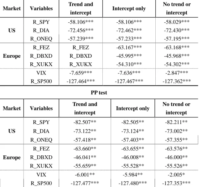
The unit root test for the endogenous and exogenous variables are summarized in Table 3. The Augmented Dickey-Fuller (ADF) and Phillips-Perron (PP) tests were used to explore the existence of unit roots in the individual returns series. The ADF test accommodates serial correlation by specifying explicitly the structure of serial correlation in the error, but the non-parametric PP test allows fairly mild assumptions that do not assume a specific type of serial correlation and heteroskedasticity in the disturbances, and can have higher power than the ADF test under a wide range of circumstances.

The null hypothesis of the ADF and PP tests is that the series have a unit root (Dickey and Fuller, 1979; Phillips and Perron, 1988). In Table 3, based on the ADF and PP test results, the large negative values in all cases indicate rejection of the null hypothesis at the 1% level of significance, which suggests that each of the ETFs returns series is

stationary.

[Insert Table 3 here]

5. Empirical Results

Tables 4 and 5 report the dynamic relationships among three ETFs, as well as the effects of exogenous variables, such VIX on the ETF returns, for the European market. In order to examine the short-term and long-terms effect of VIX on ETF returns, we incorporate the single day rate of change in VIX (followed by the S&P 500 index), the 10-day average rate of change in VIX (followed by the S&P 500 index), and the 20-day average rate of change in the VIX (followed by S&P 500 index) in the alternative models. In Table 6, we replace the VIX returns with the S&P 500 index returns as an exogenous variables, and compare their respective effects.

5.1 ETFs in the European market

Table 4 reports the results of estimating the VAR model on the returns of the three European market ETFs, namely FEX, DBXD, and XUKX, that track the underlying indexes for the EURO STOXX50 INDEX, German DAX Index, and FTSE 100 Index, respectively.

It can be seen that the returns for the three European ETFs in the previous period are significantly negatively correlated with the returns in the current period, where the negative impact of the returns of the XUKX in the previous period on those in the current period is the greatest, the value of the coefficient being -0.392. In addition to

the presence of autocorrelation in the variables, as to whether the ETF returns which tracked different indicators were characterized by mutually interactive dynamic behavior, for the VAR model, FEZ returns lagged one period were significant in terms of their ability to explain the returns of the other two ETFs.

FEZ returns lagged one period had a significant positive influence on DBXD returns in the current period, the coefficient being 0.117, and also had a significant positive influence on the XUKX returns in the current period, the coefficient being 0.173. However, XUKX returns lagged one period only significantly explained DBXD returns in the current period, the coefficient being -0.132.

Thus, it can be inferred that FEZ returns had significant explanatory power in relation to the returns in the current period of the other two ETFs that tracked a single country index, the reason being that the source of the stocks that made up the FEZ was the EURO STOXX50 INDEX, that is, an index of the markets for Europe. In this way, it was relatively easy to select large-valued stocks from the same industries as those for DBXD and XUKX. In addition, these large-valued stocks for different industries were correlated with each other through the ETF returns.

It is worth noting that the negative impact of the rates of change of VIX on the returns to XUKX ETF are both significant and persistent, while the returns of FEZ are the least affected by the rates of change in VIX. The single day rate of change in VIX in the previous period has a significant negative impact on the return of XUKX in the current period, the coefficient being -0.026. The 10-day average rate of change in VIX also had a significant negative impact on the return of XUKX in the current period, the coefficient being -0.054.

However, when the moving average is extended from 10 to 20 days, the 20-day moving average rate of returns in VIX does not have a significant impact on the return of XUKX in the current period. The rate of change in VIX in the previous period has a significant negative impact on the return of DBXD in the current period, with negative coefficient -0.021, but it is not impacted by the 10-day or 20-day average rate of change in VIX. Moreover, the coefficients of VIX are negative, indicating that when the rate of change in VIX is large, this will result in a reduction in the returns on DBXD and XUKX in the following period.

In sum, the returns of the ETFs that track a single country’s stock market index tend to be influenced relatively more by the rate of change of VIX than the Euro zone stock market, but the impact of the rate of change of VIX on the ETF returns is still only temporary.

[Insert Table 4 here]

Table 5 reports the a counterpart results with the daily, 10-day and 20-day average rate of change in the returns of the S&P500 index to the returns of the three ETFs in Europe. The empirical results show that the rates of change of the S&P500 index have negative and significant impacts on the returns of FEZ, while there is a positive and significant impacts on the returns of DBXD and XUKX, respectively.

In addition, the single day rate of change in S&P500 in the previous period has a significant positive impact on the return of XUKX in the current period, with positive coefficient 0.502. The 10-day average rate of change in VIX shows a less significant

positive impact on the return of XUKX, with positive coefficient 0.228. However, when the period of the moving average is extended from 10 to 20 days, the 20-day average rate of change in the S&P 500 index does not have a significant impact on the return of XUKX in the current period.

The rate of change in S&P500 in the previous period has a significant positive impact on the return of DBXD in the current period, with positive coefficient 0.346, but DBXD is not impacted by the 10-day or 20-day average rate of change in S&P500. Moreover, the coefficients of S&P500 are positive, indicating that larger positive returns in the S&P500 index in the current period will cause an increase in the returns on DBXD and XUKX in the next period.

[Insert Table 5 here]

5.2. ETFs in the US market

Table 6 reports the results of estimation of the VAR model on the returns of the two US market ETFs, namely DIA and ONEQ, that track the underlying indexes for the DJIA and Nasdaq Composite indexes. However, as VIX is based on call and put S&P500 index option premium prices to obtain indirectly the weighted average of the implied volatility series, we exclude SPY that tracks the underlying indexes for the S&P500 index from the VAR system for the US market in order to reduce the problem of possible measurement error.

The returns for the two U.S. ETFs in the previous period are significantly negatively correlated with the returns in the current period, where the negative impact of the

returns of DIA in the previous period on those in the current period is the greatest, with negative coefficient -0.145. However, there is no significant mutually interactive dynamic behavior in the VAR model, with DIA returns lagged one period having no impact on the returns of ONEQ ETFs, and vice-versa.

The single day rate of change in VIX in the previous period has no impact on the return of DIA in the current period. Similarly, there is no impact from either the 10-day or 20-day average rate of change in VIX on the returns of DIA in the current period. Moroever, the single day rate of change in VIX in the previous period, and both the 10-day and 20-day average rates of change in VIX have no significant impact on ONEQ in the current period.

[Insert Table 6 here]

5.3 Testing and Correcting for Conditional Heteroskedasticity

As mentioned in Section 3.1 in testing for multivariate conditional heteroskedasticity, the results of multivariate ARCH-LM tests are given in Table 7. The results show the shocks of returns of ETFs significantly reject the null hypothesis that 𝑩𝑩_𝟏𝟏 is equal to zero at the 1% level of significance.

Tables 8 and 9 report the results of the estimation of the VAR model on three returns of the European ETFs by using the diagonal BEKK model to correct for the conditional heteroscedasticity, with Table 8 presenting the results of VAR and Table 9 presenting the results of diagonal BEKK.

The single day rate of change in VIX in the previous period has a significant negative impact on the return of XUKX in the current period, with negative coefficient -0.037. The 10-day average rate of change in VIX also has a significant negative impact on the return of XUKX in the current period, with negative coefficient -0.032. The rate of change in VIX in the previous period has a significant negative impact on the return of DBXD in the current period, with negative coefficient -0.028, but it is not impacted by the 10-day or 20-day average rates of change in VIX. However, the rates of change in VIX has no significant impact on the returns of FEZ in the current period.

[Insert Tables 7, 8 and 9 here]

Tables 10 and 11 report the results of estimation of the VAR model on the three returns of ETFs in the US market by using the diagonal BEKK model to correct for the conditional heteroscedasticity, with Table 10 presenting the results of VAR and Table 11 presenting the results of diagonal BEKK. The empirical results show that the rate of change in VIX in the previous period has no impact on the returns of ETFs in the US market. The reason for VIX having no significant impact on the ETFs in the US market might arise because VIX and the lagged market index ETFs are highly correlated due to overlapping information sets.

[Insert Tables 10 and 11 here]

6. Conclusion

The purpose of this paper was to analyze the linkages of VIX and ETF returns, where the relationships in volatility returns do not yet seem to have been investigated in the

literature. Vector autoregressive (VAR) models are used to determine whether daily VIX returns with different moving average processes affect ETF returns. Moreover, the ARCH-LM test shows that there is conditional heteroskedasticity in the ETF returns, so the diagonal BEKK model is estimated to accommodate the conditional heteroskedasticity in the VAR estimates of ETF returns.

The daily ETFs are investigated to track three major US stock market indexes, namely SPY, DIA and ONEQ, as well as the ETFs for three major European stock market indexes, namely FEZ, DBXD and XUKX. The daily closing prices for each of the ETF variables are sourced from Yahoo Finance, while the VIX data are sourced from the official CBOE website.

The empirical results show that VIX has a stronger significant effect on single market ETF returns than on European market ETF returns. VIX daily returns have a stronger significant impact on European market ETF returns in the short run. Finally VIX has lower impact on the ETF returns than S&P500 returns. However, in the US market, VIX and lagged market index ETFs are highly correlated due to overlapping information sets.

Table 1 Sample Periods

Endogenous variables

Market ETFs Benchmark Index Sample Time

US

SPY S&P 500 1993.01.29～2015.03.30

DIA DJIA 1998.01.20～2015.03.30

ONEQ NASDAQ 2003.10.01～2015.03.30

Europe

FEZ EURO STOXX50 2002.10.21～2015.03.30

DBXD German DAX 2007.01.17～2015.03.30

XUKX FTSE100 2007.09.06～2015.03.30

Exogenous variables

VIX 1990.01.02～2015.03.30

S&P 500 1993.01.29～2015.03.30

Data source: ETF Database, https://beta.finance.yahoo.com/ accessed 1/10/2015.

Table 2 Sample Statistics

Endogenous variables

USA Europe

ETF R_SPY R_DIA R_ONEQ R_FEZ R_DBXD R_XUKX

Mean 0.034 0.025 0.036 -0.005 0.023 0.013 Median 0.038 0.033 0.082 0.000 0.036 0.000 Maximum 13.558 12.710 10.022 16.169 11.148 13.840 Minimum -10.364 -9.874 -8.181 -12.142 -8.038 -21.575 Std. Dev. 1.175 1.294 1.409 2.052 1.473 1.521 Skewness -0.107 0.386 -0.200 -0.008 -0.098 -2.221 Kurtosis 13.585 17.709 8.336 9.355 8.603 47.260 Exogenous variables R_VIX R_S&P500 Mean -0.025 0.017 Median -0.323 0.036 Maximum 40.547 10.957 Minimum -35.059 -9.470 Std. Dev. 7.028 1.403 Skewness 0.595 -0.305 Kurtosis 6.198 12.635

Table 3 Unit Root Tests

ADF test Market Variables Trend and

intercept Intercept only

No trend or intercept US R_SPY -58.106*** -58.106*** -58.029*** R_DIA -72.456*** -72.462*** -72.430*** R_ONEQ -57.239*** -57.233*** -57.195*** Europe R_FEZ R_FEZ -63.167*** -63.168*** R_DBXD R_DBXD -45.995*** -45.968*** R_XUKX R_XUKX -54.310*** -54.302*** VIX -7.659*** -7.636*** -2.847*** R_SP500 -127.464*** -127.467*** -127.362*** PP test Market Variables Trend and

intercept Intercept only

No trend or intercept US R_SPY -82.507** -82.505** -82.211** R_DIA -73.122** -73.124** -73.002** R_ONEQ -57.418** -57.403** -57.355** Europe R_FEZ -63.660** -63.655** -63.576** R_DBXD -46.041** -46.008** -46.000** R_XUKX -55.659** -55.528** -55.526** VIX -6.001** -5.984** -2.005* R_SP500 -127.477*** -127.480*** -127.353***

Table 4

Europe Market ETF and VIX VAR

Variables R_FEZ R_DBXD R_XUKX

R_FEZ(-1) -0.083* (0.039) 0.117** (0.027) 0.173** (0.027) R_DBXD(-1) 0.097 (0.056) -0.068 (0.040) 0.018 (0.039) R_XUKX(-1) -0.035 (0.045) -0.132** (0.032) -0.392** (0.031) C -0.006 (0.046) 0.025 (0.032) 0.017 (0.032) R_VIX(-1) 0.020 (0.009) -0.021** (0.007) -0.026** (0.006) R10_VIX(-1) 0.049 (0.037) -0.016 (0.026) -0.054* (0.026) R20_VIX(-1) -0.038 (0.055) -0.049 (0.039) -0.006 (0.039)

Note: ** and * denote significance at 1% and 5%, respectively. Standard errors are in parentheses. Table 5

Europe Market ETF and S&P 500 VAR

Variables R_FEZ R_DBXD R_XUKX

R_FEZ(-1) -0.047 (0.052) -0.038 (0.037) -0.064 (0.035) R_DBXD(-1) 0.104 (0.056) -0.050 (0.039) 0.042 (0.038) R_XUKX(-1) -0.031 (0.045) -0.145** (0.032) -0.415** (0.031) C -0.001 (0.046) 0.020 (0.032) 0.007 (0.031) R_SP500(-1) -0.137** (0.069) 0.346** (0.049) 0.502** (0.047) R10_SP500(-1) -0.332 (0.176) -0.006 (0.124) 0.228 (0.120) R20_SP500(-1) 0.135 (0.246) 0.071 (0.172) -0.145 (0.167)

Table 6

US Market ETF and VIX VAR

Variables R_DIA R_ONEQ

R_DIA(-1) -0.139** (0.039) 0.035 (0.044) R_ONEQ(-1) 0.052 (0.034) -0.087* (0.039) C 0.033 (0.020) 0.038 (0.023) R_VIX(-1) 0.002 (0.005) -0.004 (0.005) R10_VIX(-1) 0.027 (0.018) 0.019 (0.020) R20_VIX(-1) -0.019 (0.026) -0.027 (0.030)

Note: ** and * denote significance at 1% and 5%, respectively. Standard errors are in parentheses.

Table 7

ARCH-LM Tests for European and US Market ETF Returns

Europe 𝛆𝛆�_{𝐑𝐑_𝐅𝐅𝐅𝐅𝐅𝐅𝐭𝐭} 𝛆𝛆�_{𝐑𝐑_𝐃𝐃𝐁𝐁𝐃𝐃𝐃𝐃𝐭𝐭} 𝛆𝛆�_{𝐑𝐑_𝐃𝐃𝐗𝐗𝐗𝐗𝐃𝐃𝐭𝐭} LM statistic 38.819* (0) 28.254* (0) 321.64* (0) US 𝛆𝛆�_{𝐑𝐑_𝐃𝐃𝐃𝐃𝐀𝐀𝐭𝐭} 𝛆𝛆�_{𝐑𝐑_𝐎𝐎𝐎𝐎𝐅𝐅𝐎𝐎𝐭𝐭} LM statistic 97.495* (0) 129.692* (0)

Table 8

Mean Equation for European Market ETF and VIX

Variables R_FEZ R_DBXD R_XUKX

R_FEZ(-1) -0.218** (0.032) -0.005 (0.023) -0.038* (0.019) R_DBXD(-1) 0.183** (0.036) 0.011 (0.026) -0.045* (0.021) R_XUKX(-1) 0.019 (0.033) -0.086** (0.021) -0.081** (0.020) CONSTANT 0.063 (0.033) 0.087** (0.024) 0.083** (0.019) R_VIX(-1) 0.000 (0.006) -0.028** (0.004) -0.037** (0.004) R10_VIX(-1) -0.003 (0.025) -0.017 (0.019) -0.032* (0.015) R20_VIX(-1) 0.058 (0.041) -0.039 (0.031) 0.046 (0.025)

Note: ** and * denote significance at 1% and 5%, respectively. Standard errors are in parentheses.

Table 9

Diagonal BEKK for Europe Market ETF returns

Variables C A B R_FEZ 0.264* (0.023) 0.275* (0.013) -0.951* (0.004) R_DBXD 0.174* (0.017) 0.176* (0.010) 0.292* (0.014) -0.940* (0.004) R_XUKX 0.247* (0.021) 0.139* (0.023) 0.000 (0.059) 0.499* (0.017) -0.858* (0.008)

Table 10

Mean Equation for US Market ETF and VIX

Variables R_DIA R_ONEQ

R_DIA(-1) 0.041 (0.035) 0.128** (0.043) R_ONEQ(-1) -0.044* (0.025) -0.117** (0.032) CONSTANT 0.064** (0.015) 0.076** (0.019) R_VIX(-1) 0.001 (0.004) -0.006 (0.004) R10_VIX(-1) 0.010 (0.012) 0.006 (0.014) R20_VIX(-1) 0.009 (0.019) 0.010 (0.024)

Note: ** and * denote significance at 1% and 5%, respectively. Standard errors are in parentheses.

Table 11

Diagonal BEKK for US Market ETF returns

Variables C A B R_DIA 0.138* (0.010) 0.270* (0.012) 0.949* (0.005) R_ONEQ 0.126* (0.010) 0.071* (0.008) 0.229* (0.011) 0.964* (0.003)

Figure 1

VIX and S&P 500 (SPX)

0 70 140 210 0 30 60 90

ene-90 ene-95 ene-00 ene-05 ene-10 ene-15

SPX

VIX

VIX SPY

High close 80.86 on 20-Nov-08

Figure 2

Exogenous Variables: Returns on VIX and S&P 500

a. VIX Daily Returns a. SP500 Daily Returns

b. VIX 10-day average daily return b. SP500 10-day average Daily Returns

c. VIX 20-day average daily return c. SP500 20-day average Daily Returns

1990 1992 1994 1996 1998 2000 2002 2004 2006 2008 2010 2012 2014 -40 -30 -20 -10 0 10 20 30 40 50 1950 1955 1960 1965 1970 1975 1980 1985 1990 1995 2000 2005 2010 2015 -25 -20 -15 -10 -5 0 5 10 15 1990 1992 1994 1996 1998 2000 2002 2004 2006 2008 2010 2012 2014 -6 -4 -2 0 2 4 6 8 10 1950 1955 1960 1965 1970 1975 1980 1985 1990 1995 2000 2005 2010 2015 -4 -3 -2 -1 0 1 2 1990 1992 1994 1996 1998 2000 2002 2004 2006 2008 2010 2012 2014 -4 -2 0 2 4 6 1950 1955 1960 1965 1970 1975 1980 1985 1990 1995 2000 2005 2010 2015 -2.0 -1.5 -1.0 -0.5 0.0 0.5 1.0 1.5

Figure 3 VIX and ETF

US Market ETF

Eurpopean Market ETF VIX 1990 1992 1994 1996 1998 2000 2002 2004 2006 2008 2010 2012 2014 0 10 20 30 40 50 60 70 80 90 25 50 75 100 125 150 175 200 225 VIX SPY DIA ONEQ VIX 1990 1992 1994 1996 1998 2000 2002 2004 2006 2008 2010 2012 2014 0 10 20 30 40 50 60 70 80 90 0 20 40 60 80 100 120 VIX FEZ DBXD XUKX

References

Arik, A. (2011), Modeling Market Sentiment and Conditional Distribution of Stock Index Returns under GARCH Process, Ph.D. Dissertation, Department of Economics, Claremont Graduate University.

Baba, Y., R.F. Engle, D. Kraft and K.F. Kroner (1985), Multivariate Simultaneous Generalized ARCH. Unpublished manuscript, Department of Economics, University of California, San Diego, CA, USA.

Black, F. (1976), Studies of Stock Market Volatility Changes, in Proceedings of the American Statistical Association, Business and Economic Statistics Section, Washington, DC, USA, pp. 177-181.

Bollerslev, T. (1986), Generalized Autoregressive Conditional Heteroskedasticity,

Journal of Econometrics, 31, 307-327.

Bollerslev, T. (1990), Modelling the Coherence in Short-run Nominal Exchange Rate: A Multivariate Generalized ARCH Approach, Review of Economics and Statistics, 72, 498-505.

Borovkova, S. and F.J. Permana (2009), Implied Volatility in Oil Markets,

Computational Statistics and Data Analysis, 53, 2022-2039.

Boussama, F. (2000), Asymptotic Normality for the Quasi-maximum Likelihood

Estimator of a GARCH Model, Comptes Rendus de l’Academie des Sciences, 331,

81-84.

Caporin, M. and M. McAleer (2012), Do We Really Need both BEKK and DCC? A Tale of Two Multivariate GARCH Models, Journal of Economic Surveys, 26(4), 736-751.

Caporin, M. and M. McAleer (2013), Ten Things You Should Know About the Dynamic Conditional Correlation Representation, Econometrics, 1(1), 115-126. Chang, C.-L., Y. Li, and M. McAleer (2015), Volatility Spillovers between Energy and

Agricultural Markets: A Critical Appraisal of Theory and Practice, Tinbergen Institute Discussion Papers 15-077/III, Tinbergen Institute.

Chang, C.-L. and M. McAleer (2015) (eds.), Econometric Analysis of Financial Derivatives, Journal of Econometrics, 187(2), 403-633.

Cochran, S.J., I. Mansur, and B. Odusami (2015), Equity Market Implied Volatility

and Energy Prices: A Double Threshold GARCH Approach, Energy Economics,