San Jose State University
SJSU ScholarWorks
Mineta Transportation Institute Publications
8-2015
Development of Bus-Stop Time Models in Dense
Urban Areas: A Case Study in Washington DC
Stephen Arhin
Howard University
Errol Noel
Howard University
Follow this and additional works at:http://scholarworks.sjsu.edu/mti_publications Part of theTransportation Commons
This Report is brought to you for free and open access by SJSU ScholarWorks. It has been accepted for inclusion in Mineta Transportation Institute Publications by an authorized administrator of SJSU ScholarWorks. For more information, please contactscholarworks@sjsu.edu.
Recommended Citation
Stephen Arhin and Errol Noel. "Development of Bus-Stop Time Models in Dense Urban Areas: A Case Study in Washington DC"
Development of Bus-Stop Time
Models in Dense Urban Areas:
A Case Study in Washington DC
MNTRC Report 12-48
Funded by U.S. Departmentof Transportation MNTRC Lo ng -T er m T re nd s i n P at ro n S at isf ac tio n o f D C C irc ula to r M T I R epo rt 1 2-09 Oc to be r 2 01 3
MNTRC
MINETA NATIONAL TRANSIT RESEARCH CONSORTIUM
The Mineta Transportation Institute (MTI) was established by Congress in 1991 as part of the Intermodal Surface Transportation Equity Act (ISTEA) and was reauthorized under the Transportation Equity Act for the 21st century (TEA-21). MTI then successfully
competed to be named a Tier 1 Center in 2002 and 2006 in the Safe, Accountable, Flexible, Efficient Transportation Equity Act: A
Legacy for Users (SAFETEA-LU). Most recently, MTI successfully competed in the Surface Transportation Extension Act of 2011 to be named a Tier 1 Transit-Focused University Transportation Center. The Institute is funded by Congress through the United States
Department of Transportation’s Office of the Assistant Secretary for Research and Technology (OST-R), University Transportation
Centers Program, the California Department of Transportation (Caltrans), and by private grants and donations.
The Institute receives oversight from an internationally respected Board of Trustees whose members represent all major surface transportation modes. MTI’s focus on policy and management resulted from a Board assessment of the industry’s unmet needs and led directly to the choice of the San José State University College of Business as the Institute’s home. The Board provides policy direction, assists with needs assessment, and connects the Institute and its programs with the international transportation community.
MTI’s transportation policy work is centered on three primary responsibilities:
MINETA TRANSPORTATION INSTITUTE
LEAD UNIVERSITY OF MNTRC
Research
MTI works to provide policy-oriented research for all levels of government and the private sector to foster the development
of optimum surface transportation systems. Research areas in
-clude: transportation security; planning and policy development;
interrelationships among transportation, land use, and the
environment; transportation finance; and collaborative labor-management relations. Certified Research Associates conduct the research. Certification requires an advanced degree, gener -ally a Ph.D., a record of academic publications, and
profession-al references. Research projects culminate in a peer-reviewed
publication, available both in hardcopy and on TransWeb,
the MTI website (http://transweb.sjsu.edu).
Education
The educational goal of the Institute is to provide graduate-lev-el education to students seeking a career in the devgraduate-lev-elopment and operation of surface transportation programs. MTI, through San José State University, offers an AACSB-accredited Master of
Science in Transportation Management and a graduate Certifi -cate in Transportation Management that serve to prepare the na-tion’s transportation managers for the 21st century. The master’s degree is the highest conferred by the California State
Univer-sity system. With the active assistance of the California Department of Transportation, MTI delivers its classes over a state-of-the-art videoconference network throughout the state of California and via webcasting beyond, allowing working transportation professionals to pursue an advanced degree regardless of their location. To meet the needs of employers seeking a diverse workforce, MTI’s education program promotes enrollment to under-represented groups.
Information and Technology Transfer
MTI promotes the availability of completed research to professional organizations and journals and works to
integrate the research findings into the graduate education
program. In addition to publishing the studies, the Institute also sponsors symposia to disseminate research results
to transportation professionals and encourages Research Associates to present their findings at conferences. The
World in Motion, MTI’s quarterly newsletter, covers innovation in the Institute’s research and education pro-grams. MTI’s extensive collection of transportation-related publications is integrated into San José State University’s world-class Martin Luther King, Jr. Library.
The contents of this report reflect the views of the authors, who are responsible for the facts and accuracy of the information presented herein. This document is disseminated under the sponsorship of the U.S. Department of Transportation, University Transportation Centers Program and the California Department of Transportation, in the interest of information exchange. This report does not necessarily reflect the official views or policies of the U.S. government, State of California, or the Mineta Transportation Institute, who assume no liability
DISCLAIMER
MTI FOUNDER
Hon. Norman Y. Mineta
MTI/MNTRC BOARD OF TRUSTEES
Karen Philbrick, Ph.D. Executive Director Hon. Rod Diridon, Sr. Emeritus Executive Director
Directors
MNTRC
MINETA NATIONAL TRANSITPeter Haas, Ph.D. Education Director Donna Maurillo Communications Director
Brian Michael Jenkins
National Transportation Safety and Security Center Asha Weinstein Agrawal, Ph.D.
National Transportation Finance Center Founder, Honorable Norman
Mineta (Ex-Officio)
Secretary (ret.), US Department of Transportation
Vice Chair
Hill & Knowlton, Inc.
Honorary Chair, Honorable Bill Shuster (Ex-Officio)
Chair
House Transportation and Infrastructure Committee United States House of Representatives
Honorary Co-Chair, Honorable Peter DeFazio (Ex-Officio)
Vice Chair
House Transportation and Infrastructure Committee United States House of Representatives
Chair, Nuria Fernandez (TE 2017)
General Manager and CEO Valley Transportation Authority
Vice Chair, Grace Crunican (TE 2016)
General Manager
Bay Area Rapid Transit District
Executive Director, Karen Philbrick, Ph.D.
Mineta Transportation Institute San José State University
Joseph Boardman (Ex-Officio)
Chief Executive Officer
Amtrak
Anne Canby (TE 2017)
Director OneRail Coalition
Donna DeMartino (TE 2018)
General Manager and CEO San Joaquin Regional Transit District
William Dorey (TE 2017)
Board of Directors Granite Construction, Inc.
Malcolm Dougherty (Ex-Officio)
Director
California Department of Transportation
Mortimer Downey* (TE 2018)
President
Mort Downey Consulting, LLC
Rose Guilbault (TE 2017)
Board Member
Peninsula Corridor Joint Powers Board (Caltrain)
Ed Hamberger (Ex-Officio)
President/CEO
Association of American Railroads
Steve Heminger* (TE 2018)
Executive Director Metropolitan Transportation Commission
Diane Woodend Jones (TE 2016)
Principal and Chair of Board Lea+Elliot, Inc.
Will Kempton (TE 2016)
Executive Director Transportation California
Art Leahy (TE 2018)
CEO Metrolink
Jean-Pierre Loubinoux (Ex-Officio)
Director General
International Union of Railways (UIC)
Michael Melaniphy (Ex-Officio)
President and CEO
American Public Transportation Association (APTA)
Abbas Mohaddes (TE 2018)
CEO
The Mohaddes Group
Jeff Morales (TE 2016)
CEO
California High-Speed Rail Authority
David Steele, Ph.D. (Ex-Officio)
Dean, College of Business San José State University
Beverley Swaim-Staley (TE 2016)
President
Union Station Redevelopment Corporation
Michael Townes* (TE 2017)
Senior Vice President Transit Sector, HNTB
Bud Wright (Ex-Officio)
Executive Director
American Association of State
Highway and Transportation Officials
(AASHTO)
Edward Wytkind (Ex-Officio)
President
Transportation Trades Dept., AFL-CIO
(TE) = Term Expiration or Ex-Officio
A publication of
Mineta National Transit
Research Consortium
College of BusinessREPORT 12-48
DEVELOPMENT OF BUS-STOP TIME MODELS IN
DENSE URBAN AREAS: A CASE STUDY IN
WASHINGTON DC
Stephen Arhin, Ph.D., P.E., PTOE, PMP Errol Noel, Ph.D., P.E.
TECHNICAL REPORT DOCUMENTATION PAGE
1. Report No. 2. Government Accession No. 3. Recipient’s Catalog No.
4. Title and Subtitle 5. Report Date
6. Performing Organization Code
7. Authors 8. Performing Organization Report
9. Performing Organization Name and Address 10. Work Unit No.
11. Contract or Grant No.
12. Sponsoring Agency Name and Address 13. Type of Report and Period Covered
14. Sponsoring Agency Code
15. Supplemental Notes
16. Abstract
17. Key Words 18. Distribution Statement
19. Security Classif. (of this report) 20. Security Classif. (of this page) 21. No. of Pages 22. Price
81 CA-MNTRC-15-1239
Development of Bus-Stop Time Models in Dense Urban Areas: A Case Study in Washington DC
August 2015
MNTRC Report 12-48 Stephen Arhin, Ph.D., P.E., PTOE, PMP and Errol Noel, Ph.D., P.E.
Mineta National Transit Research Consortium College of Business
San José State University San José, CA 95192-0219
U.S. Department of Transportation
Office of the Assistant Secretary for
Research and Technology
University Transportation Centers Program 1200 New Jersey Avenue, SE
Washington, DC 20590
Final Report
Unclassified Unclassified
No restrictions. This document is available to the public through
The National Technical Information Service, Springfield, VA 22161
DTRT12-G-UTC21
$15.00 Total bus stop time; Dwell time;
Optimization; Transit bus; Time of day
Bus transit reliability depends on several factors including the route of travel, traffic conditions, time of day, and conditions at
the bus stops along the route. The number of passengers alighting or boarding, fare payment method, dwell time (DT), and the
location of the bus stop also affect the overall reliability of bus transit service. This study defines a new variable, Total Bus Stop Time (TBST) which includes DT and the time it takes a bus to safely maneuver into a bus stop and the re-entering the main traffic
stream. It is thought that, if the TBST is minimized at bus stops, the overall reliability of bus transit along routes could be improved. This study focused on developing a TBST model for bus stops located near intersections and at mid-blocks using ordinary least
squares method based on data collection at 60 bus stops, 30 of which were near intersections while the remaining were at mid-blocks in Washington DC. The field data collection was conducted during the morning, mid-day, and evening peak hours.
The following variables were observed at each bus stop: bus stop type, number of passengers alighting or boarding, DT, TBST, number of lanes on approach to the bus stop, presence of parking, and bus pad length. The data was analyzed and all statistical
inferences were conducted based on 95% confidence interval. The results show that the TBST could be used to aid in improving
planning and scheduling of transit bus systems in an urban area. Howard University
Transportation Research Center
2300 6th Street, NW, Room 2121
To order this publication, please contact:
Mineta National Transit Research Consortium College of Business
San José State University San José, CA 95192-0219
Tel: (408) 924-7560 Fax: (408) 924-7565
Email: mineta-institute@sjsu.edu
transweb.sjsu.edu/mntrc/index.html
by Mineta National Transit Research Consortium
All rights reserved
Library of Congress Catalog Card Number: Copyright © 2015
iv
ACKNOWLEDGMENTS
The authors and students at the Howard University Transportation Research and Data Center would like to thank the Mineta Transportation Institute, particularly Executive Director Karen Philbrick, Ph.D. The authors would also like to thank Director of Communications and Technology Transfer Donna Maurillo; Research Support Coordinator Joseph Mercado; and Webmaster Frances Cherman, who also provided additional editorial support.
Disclaimer:
The contents of this report reflect the views of the authors, who are responsible for the facts and the accuracy of the information presented. This document is disseminated under the sponsorship of the U.S. Department of Transportation’s University Transportation Centers Program, in the interest of information exchange. The U.S. Government assumes no liability for the contents or use thereof.
v
TABLE OF CONTENTS
Executive Summary 1 TBST Models 3 DT Models 3 I. Introduction 5II. Research Objectives 6
III. Literature Review 7
Summary 11
IV. Research Methodology 12
Bus Stops Selected for the Study 12
Computing DT and TBST 14
Statistical Analyses, Regression Analyses, and Optimization 14
V. Results 19
Statistical Analysis 19
Regression Analysis 21
Model Validation 24
Optimization 26
VI. Discussion of Results 28
VII. Conclusions and Recommendations 30
Appendix 1: Bus Stop Locations 31
Appendix 2: Data Collection Sheets 33
Field Data Collection Scheme for TBST Project 33
Appendix 3: Descriptive Statistics 35
Appendix 4: Regression Analyses 38
Appendix 5: Model Validation 50
Bus Stops Located at Intersections 51
Midblock Bus Stops 57
Optimization 63
Kolmogorov-Smirnov Test 69
vi Table of Contents
Bibliography 77
About the Authors 79
vii
LIST OF FIGURES
1. Bus Stopping Zone in London’s iBus System 9
2. Selected Bus Stop Locations in the District of Columbia 13
3. Mean DT Values by Time of Day by Bus Stop Location-type 20
4. Mean TBST Values by Time of Day by Bus Stop Location-type 21
5. Residual Plot for Bus Stops Located at Intersections (Midday) 24
6. Normal Probability Plot for Bus Stops Located at Intersections (Midday) 25 7. KS-test Comparison Percentile Plot for Bus stops Located at Intersections
for TBST (Midday) 25
8. KS-test Comparison Percentile Plot for Bus stops Located at Intersections
for DT (Midday) 26
9. Data Collection Sheet for TBST Project 34
10. Intersections - TBST AM vs. Order 51
11. Intersections - TBST AM vs. Fits 51
12. Intersections - TBST AM Histogram 51
13. Intersections - TBST AM Normal Probability Plot 51
14. Intersections - TBST Midday vs. Order 52
15. Intersections - TBST Midday Histogram 52
16. Intersections - TBST PM vs. Order 53
17. Intersections - TBST PM vs. Fits 53
18. Intersections - TBST PM Histogram 53
19. Intersections - TBST PM Normal Probability Plots 53
20. Intersections - DT AM vs. Order 54
21. Intersections - DT AM vs. Fits 54
viii List of Figures
23. Intersections - DT AM Normal Probability Plot 54
24. Intersections - DT Midday vs. Order 55
25. Intersections - DT Midday vs. Fits 55
26. Intersections - DT Midday Histogram 55
27. Intersections - DT Midday Normal Probability Plot 55
28. Intersections - DT PM vs. Order 56
29. Intersections - DT PM vs. Fits 56
30. Intersections - DT PM Histogram 56
31. Intersections - DT PM Normal Probability Plot 56
32. Midblock - TBST AM vs. Order 57
33. Midblock - TBST AM vs. Fits 57
34. Midblock - TBST AM Histogram 57
35. Midblock - TBST AM Normal Probability Plots 57
36. Midblock - TBST Midday vs. Order 58
37. Midblock - TBST MID vs. Fits 58
38. Midblock - TBST Midday Histogram 58
39. Midblock - TBST Midday Normal Probability Plot 58
40. Midblock - TBST PM vs. Order 59
41. Midblock - TBST PM vs. Fits 59
42. Midblock - TBST PM Histogram 59
43. Midblock - TBST PM Normal Probability Plot 59
44. Midblock - DT AM vs. Order 60
45. Midblock - DT AM vs. Fits 60
46. Midblock - DT AM Histogram 60
ix List of Figures
48. Midblock - DT Midday vs. Order 61
49. Midblock - DT Midday vs. Fits 61
50. Midblock - DT MID Histogram 61
51. Midblock - DT MID Normal Probability Plot 61
52. Midblock - DT PM vs. Order 62
53. Midblock - DT PM vs. Fits 62
54. Midblock - DT PM Histogram 62
55. Midblock - DT PM Normal Plot 62
56. Intersections - TBST AM Optimization Output 64
57. Intersections - TBST MID Optimization Output 65
58. Intersections - TBST PM Optimization Output 66
59. Midblock - TBST AM Optimization Output 67
60. Midblock - TBST MID Optimization Output 68
61. Midblock - TBST PM Optimization Output 69
62. Intersections - TBST AM K-S Test Comparison Percentile Plot 70
63. Intersections - TBST PM K-S Test Comparison Percentile Plot 70
64. Intersections - DT AM K-S Test Comparison Percentile Plot 71
65. Intersections - DT PM K-S Test Comparison Percentile Plot 71
66. Midblock - TBST AM K-S Test Comparison Percentile Plot 72
67. Midblock - TBST MID K-S Test Comparison Percentile Plot 72
68. Midblock - TBST PM K-S Test Comparison Percentile Plot 73
69. Midblock - DT AM K-S Test Comparison Percentile Plot 73
70. Midblock - DT MID K-S Test Comparison Percentile Plot 74
x
LIST OF TABLES
1. Summary of TBST Regression Analysis by Time of Day at Intersections 3 2. Summary of TBST Regression Analysis by Time of Day at Midblock 3 3. Summary of DT Regression Analysis by Time of Day at Intersections 3
4. Summary of DT Regression Analysis by Time of Day at Midblock 3
5. Maximum TBST 4
6. Summary of Developed Models 11
7. Summary of Descriptive Statistics for Midblock Bus Stops 19
8. Summary of Descriptive Statistics for Bus Stops Located at Intersections 20 9. Summary of TBST Regression Analysis by Time of Day at Intersections 23 10. Summary of TBST Regression Analysis by Time of Day at Midblock 23 11. Summary of DT Regression Analysis by Time of Day at Intersections 23
12. Summary of DT Regression Analysis by Time of Day at Midblock 23
13. Summary of Optimal TBST 27
14. Locations of Bus Stops at Intersections 31
15. Locations of Midblock Bus Stops 32
16. Descriptive Statistics for Variables Collected at Intersections – AM 35 17. Descriptive Statistics for Variables Collected at Intersections – Midday 35 18. Descriptive Statistics for Variables Collected at Intersections – PM 36 19. Descriptive Statistics for Variables Collected at Midblock – AM 36 20. Descriptive Statistics for Variables Collected at Midblock – Midday 37 21. Descriptive Statistics for Variables Collected at Midblock – PM 37
22. Intersections – Regression Analysis TBST – AM 38
xi List of Tables
24. Intersections – Regression Analysis TBST – PM 40
25. Intersections – Regression Analysis DT – AM 41
26. Intersections – Regression Analysis DT – Midday 42
27. Intersections – Regression Analysis DT – PM 43
28. Midblock – Regression Analysis TBST – AM 44
29. Midblock – Regression Analysis TBST – Midday 45
30. Midblock – Regression Analysis TBST – PM 46
31. Midblock – Regression Analysis DT – AM 47
32. Midblock – Regression Analysis DT – Midday 48
33. Midblock – Regression Analysis DT – PM 49
34. Summary of TBST K-S Test Results 69
1
EXECUTIVE SUMMARY
The primary goal of transit agencies is to provide reliable, efficient, and productive transportation service. Transit reliability has been defined many times; for example in 1978, Abkowitz et al1 defined transit reliability as the availability and stability of transit service attributes and their effects on travel behavior and on transit agencies’ performance travel behavior and on transit agencies performance. Two years later, Turnquist and Blume2 described transit reliability as keeping transit vehicles on-schedule with uniform headways and consistent travel times. More recently, Kimple3 stated that transit reliability is a multidimensional phenomenon; consequently, there is not a single measure that can adequately address service quality.
Bus transit reliability depends on several factors, including the route of travel, traffic conditions, time of day, and conditions at the bus stops along the route. The number of passengers alighting or boarding, fare payment method, dwell time, and the location of the bus stop also affect the overall reliability of bus transit service. Several research studies have been conducted on bus dwell time (DT), which is defined as the time interval between the opening and closing of the vehicle’s doors to serve passengers at a transit stop. This study defines a new variable: Total Bus Stop Time (TBST) which, in addition to DT, includes the time required for a bus to safely maneuver into a transit stop and the time consumed reentering the main traffic stream. It is thought that if the TBST is minimized, the overall reliability of bus transit along routes could be improved.
It is clear that providing a reliable transit service is necessary in order to maintain an efficient and attractive system that increases users’ satisfaction and loyalty. Furthermore, reliable transit improves internal efficiency, reduces operating costs, and improves revenues by attracting and retaining users. Therefore, improving reliability is a benefit for both users and transit agencies, as it enables cities to achieve broader goals.
This study was aimed at developing DT and TBST models for bus stops located at intersections and at midblock. The TBST models were developed using nonlinear optimization methods. The study involved data collection at sixty bus stops, thirty of which were located at intersections, while the remaining bus stops were at midblock. The data was obtained for the morning, midday and evening peak hours during the period from January 2014 through September 2014. Data on the following variables were obtained at each bus stop: bus stop type, number of passengers alighting or boarding, DT, TBST, number of lanes on approach to the bus stop, presence of parking, and bus pad length. The data was analyzed and all statistical inferences were conducted based on 95% confidence level.
The results of the data analyzed showed that, on average, both TBST and DT were higher at bus stops at intersections than at those located midblock. While the mean TBST was approximately 48 seconds at the bus stops at intersections, for the midblock bus stops, the mean DT and TBST were 21 and 35 seconds, respectively. The overall mean DT was determined to be 29 seconds.
2 Executive Summary
The regression models for the TBST and DT were determined to be statistically significant at the 95% confidence level based on the R2, F-Statistics, and model validation tests. The models could explain 67% to 96% of the variations in the data based on the R2 and adjusted R2 values. Tests including Kolmogorov-Smirnoff, normal probability, and residual plots were used to confirm the appropriateness of the models. The models were developed by bus stop type and by time of day. The following tables present the models:
Mineta National
T
ransit Research Consortium
3
Executive Summary
TBST MODELS
Table 1. Summary of TBST Regression Analysis by Time of Day at Intersections
Time Period Model Equation R2 Adj. R2
ANOVA F-value p-value
Morning TBSTAM= 1.40(DT) -1.90(PB) -1.19(PK) + 2.45(LN) -0.001(BP) -0.02(PA) + 14.6 0.67 0.59 7.81 0.00
Midday TBSTMID= 1.12(DT) + 0.26(PB) -1.87(PK) + 0.52(LN) -0.002(BP) -0.15(PA) + 17.23 0.96 0.95 96.89 0.00
Evening TBSTPM= 1.17(DT) -0.02(PB) -1.55(PK) -2.07(LN) + 0.0002(BP) -0.42(PA) + 21.72 0.95 0.93 70.51 0.00
Table 2. Summary of TBST Regression Analysis by Time of Day at Midblock
Time Period Model Equation R2 Adj. R2
ANOVA F-value p-value Morning TBSTAM= 1.73(DT) -2.19(PB) + 3.91(PK) - 0.15(LN) + 0.002(BP) - 1.21(PA) - 0.0009 0.73 0.65 10.17 0.00 Midday TBSTMID= 1.12(DT) + 0.04(PB) - 0.86(PK) + 0.50(LN) + 0.005(BP) - 0.27(PA) + 8.71 0.98 0.97 164.16 0.00 Evening TBSTPM= 1.12(DT) + 0.19(PB) - 0.50(PK) - 0.19(LN) + 0.004(BP) - 0.07(PA) + 7.94 0.99 0.99 360.27 0.00 DT MODELS
Table 3. Summary of DT Regression Analysis by Time of Day at Intersections
Time Period Model Equation R2 Adj. R2
ANOVA F-value p-value
Morning DTAM= 3.42(PB) - 2.05(PK) - 1.34(LN) - 0.0005(BP) + 1.11(PA) + 14.13 0.73 0.67 12.82 0.00
Midday DTMID= 5.37(PB) + 7.01(PK) + 4.52(LN) + 0.002(BP) + 2.26(PA) - 20.70 0.82 0.78 21.53 0.00
Evening DTPM= 4.31(PB) -1.86(PK) + 0.29(LN) - 0.003(BP) + 2.88(PA) + 4.50 0.95 0.93 70.51 0.00
Table 4. Summary of DT Regression Analysis by Time of Day at Midblock
Time Period Model Equation R2 Adj. R2
ANOVA F-value p-value
Morning DTAM= 3.00(PB) + 4.52(PK) + 1.43(LN) - 0.004(BP) + 1.69(PA) - 1.31 0.89 0.86 37.09 0.00
Midday DTMID= 4.75(PB) - 4.61(PK) + 2.20(LN) + 0.0005(BP) + 1.05(PA)+ 8.15 0.73 0.67 13.00 0.00
4 Executive Summary
The TBST models were then optimized to yield the maximum values based on the upper confidence limits of the DTs for each bus stop type and time of day. Because DT was determined to be the independent variable with the most statistically significant impact on the TBST, this constraint was used. From the results, the following maximum TBSTs were observed for each bus stop type by time of day:
Table 5. Maximum TBST
Bus Stop Type Time Period
Maximum TBST (secs) Intersections AM 42.5 MID 47.1 PM 66.8 Midblock AM 36.0 MID 33.2 PM 31.2
The results suggest that to sustain or improve bus reliability at bus stops at intersections, during the morning, midday, and evening peak periods, buses should spend no more than 43, 47 and 67 seconds, respectively. Similarly, the total time at midblock bus stops should be no more than 36, 34, and 32 seconds, respectively.
Due to potential changes in traffic patterns and varying land uses near bus stops, the models need updating and validation on a 3-to-5-year cycle. These models are based on data that was limited to DC bus routes and street characteristics; therefore, they may not be appropriate for predicting TBST or DT in other jurisdictions.
5
I. INTRODUCTION
The overall reliability of a transit bus system depends on several factors along the route of travel. These include but are not limited to scheduled arrivals, traffic congestion, weather conditions, dwell times at bus stops, and the number of passengers boarding and alighting. Dwell time (DT) is defined as the time that a transit vehicle is stopped for the purpose of serving passengers and encompasses the total passenger service time between the opening and closing of doors.4 The DT at bus stops represents a significant portion of route operating time and its variability. It is linked to the reliability of the service being provided. Planning and managing bus schedules necessitate being able to estimate the total time buses spend at bus stops, not just the time consumed in the boarding and alighting of passengers. The time consumed in the safe maneuver of buses into a bus stop and the time required to merge back into traffic are also important elements in urban bus transit schedule development. Those times, along with the DT, comprise the total bus stop time (TBST), which is likely to be affected by bus-specific activities and systems and by traffic operational conditions along bus transit corridors and at bus stops.
Since TBST affects overall transit reliability, it is one of the variables regional bus transit systems, such as the Washington Metropolitan Area Transit Authority (WMATA), must measure. As part of its initiatives to provide timely information regarding bus arrivals and travel times, WMATA provides real-time information on bus arrival times for many routes. Patrons can use smart phones, standard computers, or a variety of other portable information devices to access the information. WMATA recently incorporated Automatic Vehicle Location (AVL) and Automatic Passenger Counting (APC) systems to improve the bus information system. The reliability of a bus route service is generally gauged by determining if the transit system is compliant with its advertised schedules. Since TBST is a factor in reliability assessments, it is critical to predict its value along bus transit corridors. This research uses data for WMATA’s bus stops along heavily traveled corridors for the purpose of developing and optimizing DT and TBST models.
6
II. RESEARCH OBJECTIVES
The demand for public transit services in the District of Columbia is driven by the steadily increasing population of residents, commuters, and visitors. The cost of automobile ownership, including the cost of gasoline and parking, has stimulated commuter interest in public transit. Consequently, there is an increasing need for more reliable transit systems in the Washington DC Metropolitan Area.
WMATA attempts to fulfill the demand by providing regional rail transit service and bus service along heavily traveled corridors in the Metropolitan Area. Both rail and bus services are monitored by WMATA via its protocol for collecting and analyzing related data. The time it takes for a transit bus to maneuver to a stop position for passengers to alight and board and the time required for the bus to reenter traffic affect overall bus service reliability. This research is intended to develop DT and TBST models by time of the day that could be used to improve overall bus transit reliability. The following objectives form the basis of this research:
• Identify variables influencing DT and, subsequently, TBST.
• Develop DT and TBST models for bus stops at intersections and at midblock. • Optimize the TBST models to improve bus transit schedule planning and efficiency. The results will contribute toward the provision of a reliable bus transit service highly valued by the community.
7
III. LITERATURE REVIEW
There is a trend toward an increasing population density in already crowded urban areas due to thriving employment opportunities. Urban transit systems are generally recognized as both an efficient mode of travel and a strategy for reducing air pollution and dependency on petroleum-based fuels for transportation. The overall effectiveness of transit service relies heavily on the quality of the network’s routing structure, schedules, management, and reliability of service. Since urban streets pose a number of challenges for bus drivers trying to maintain schedules, a full understanding of actual-versus-anticipated travel times and the practices or events that save time or cause it to be lost during service are constant concerns of transit operators. These fluctuations are relevant both in the context of multimodal transit or single-mode transit systems, as transfers and wait times are critical to passengers. Street traffic, pedestrian and bike transport, weather, crashes, traffic control, and various curb-lane activities are among the many unpredictable conditions randomly affecting the docking and undocking of buses at curbside bus stops. The ability to effect seamless and efficient transit vehicle access and egress is one of the most significant factors used in establishing predictable transport times. In many ways predictable timing is more important than trip duration.
The docking and undocking phases of bus transit in large urban transit systems are affected by many unpredictable variables, such as the mix of street traffic, location of bus stops, turns at intersections, traffic control devices, timing/coordination of traffic control devices, physical design configuration of bus stops, and curbside parking activities, to mention a few.
Knowledge of the magnitude variability of the access, dwell, and departure intervals of transit vehicles over the entire daily service period plays a critical role in schedule design and operation management.
The authors reviewed previous studies that focused on understanding the total time involved in transit stops, including arrival, dwell time, and departure from curbside bus stops. Literature on bus dwell times and their associated models are generally sparse, and measurements in a form directly usable for our purposes do not exist. Related studies were based on small sample sizes. These studies are not directly relevant and tend to be route-specific, analyzing other issues causing bus delays.5 Some studies on dwell time have also used ordinary least squares (OLS) regression to relate dwell time to passenger boarding and alighting under selected operating conditions that were likely to affect dwell time. A study conducted by Milkovits6 developed dwell time models for heavy rail, light rail, and bus transit systems.
Kraft and Bergen7 found that passenger service time requirements for morning and evening peaks were similar, and midday requirements were greater than those in peak periods. This research determined boarding times exceed alighting times, and that rear door and front door alighting times were the same and concluded that dwell time was equal to 2 seconds plus 4.5 seconds for each boarding passenger who paid with cash and required change, and 1.5 seconds plus 1.9 seconds for each passenger who had exact fare.
8 Literature Review
Another study conducted by Kraft identified seven major groups of factors that affect dwell time: human, modal, operating policies, operating practices, mobility, climate, and other system elements.8 The study suggested that specific bus stop characteristics such as curb-lane usage, right-lane volume, right-lane configuration, vehicle classifications, gaps in traffic, parking, length of maneuvering space for the bus, could affect the time the bus spends at the bus stop.
A 1983 study conducted by Levinson9 determined that dwell time was equal to 5 seconds plus 2.75 seconds per boarding or alighting passenger. Similarly, in the same year, Guenthner and Sinha10 reported a 10- to 20-second penalty for each stop, plus a 3- to 5-second penalty for each passenger boarding or alighting. Unfortunately, both studies resulted in low explanatory power, even though the research controlled for factors such as lift activity, fare structure, and number of doors.
S. Chen, R Zhou, Y. Zhou, and B. Mao, concerned about the magnitude of bus delays at bus stops and the impact on service, conducted a field research on the behavior of buses at bayside and curbside bus stops on the streets of Beijing, China.11 The authors postulated that as a bus enters a bus stop for discharging and picking up passengers the vehicle would go through an arrival stage that would involve a careful maneuvering of the vehicle toward the designated stop position while avoiding parked vehicles, physical items, and pedestrians. That arrival pattern was conceived to be different from arrival of vehicles in bus rapid transit systems (BRT) where the guideways would be free from obstacles. The dwell times at street bus stops are usually limited to time needed for the doors to open and close in service of passengers. Leaving time was described as time between closures of the doors to the return of a bus to the traffic stream. In 2011, the researchers collected video data on twelve buses during the morning rush-hour and the period from 12 noon to 2:00 p.m. They also observed the number of passengers on board, boarding, and alighting. In total, 300 events were recorded. The researchers found that dwell time correlates with passenger activities at the doors, despite the magnitude of load factors. Boarding and alighting times for curbside bus stops were observed to increase when the load factor is greater than 0.55. The researchers recommended further work on the arrival and departure intervals at bus stops. Linear regression models were developed to estimate the expected docking time at curbside bus stops when the load factor is below 0.55 and above 0.77.
Generally, bus stop docking time for BRT is not obscured by unrelated activities near the stops. However, due to concern regarding the length of the docking period, which includes the dwell time, a study was launched in 2006 to evaluate travel time of the Metropolitan Area Express (MAX) system in Las Vegas.12 Repeated accumulation of dust and dirt on the pavement in the docking area obscured the visibility of pavement markings and stimulated interest in a technology-based solution. An optical guidance system was used to facilitate the docking of buses into bus bays, although the trained drivers demonstrated sufficient capability to park their buses into the marked bays. The guidance system involved automatic vehicle location sensors. Although the system reduced the time consumed in maneuvering buses in and out of positions at the BRT stations, management determined its cost to be prohibitive.
9 Literature Review
In 2013, S. Robinson13 conducted a study in London introducing a new metric called “time
lost serving stop” – defined as the time that typical bus would save if a bus stop were not present. That study sought to examine the impact on dwell time of time lost decelerating to serve a bus stop and accelerating to traffic speed upon leaving. Data developed here was taken from the iBus system, an Automatic Vehicle Location (AVL) system installed on more than 8,000 bus units in the city of London. The systems logged the speed, location, and odometer values of vehicles, as well as the times when doors were opened and closed. In that study, a bus was considered to be at a bus stop when it entered the stopping zone, which was defined as 50 meters before and 30 meters after the flagpole, as shown in Figure 1.
Figure 1. Bus Stopping Zone in London’s iBus System
Comparing the results using two different approaches, peak-to-peak speed and shifted speed, Robinson evaluated over 50,000 bus stop events from the iBus system to estimate the mean time lost in serving bus stops along Route 45. The peak-to-peak speed approach used the peak speed before and after the stop.
The shifted speed approach assumed that the bus would be traveling at the highest peak speed if the bus stop had not been present. Both approaches presented a directly proportional relationship between the two variables: speed and distance. The results indicated that the shifted speed approach was more realistic, and it was used to determine that the mean time lost in arriving, serving, and departing from a bus stop was 11.6 seconds – considerably longer than the time the doors would remain open.
Hooi Ling Khoo14 developed bus dwell time statistical models using dwell time data from 20 bus stops in the Klang Valley region in Malaysia in 2010 and 2011. The researcher wanted to determine the statistical distribution that could best explain and describe dwell time variability, and used regression models to assess the degree of influence of the factors considered. The bus stops selected for the study were chosen based on the type of location, number of bus routes served, and an estimation of the passenger demand. Both field crew and video recording were used to collect dwell time data for peak and off-peak hours. The off-peak hours were from 8 a.m. to 9 a.m. and from 5 p.m. to 6 p.m., while the off-peak period was from 9 a.m. to 10 a.m. and from 4 p.m. to 5 p.m.
10 Literature Review
The dwell time was computed using the following equation:
𝑡𝑡𝑖𝑖 =𝑡𝑡
𝑑𝑑𝑑𝑑𝑑𝑑𝑑𝑑𝑑𝑑𝑑𝑑𝑖𝑖 − 𝑡𝑡𝑑𝑑𝑑𝑑𝑑𝑑𝑖𝑖𝑎𝑎𝑑𝑑𝑖𝑖 where,
• 𝑡𝑡𝑖𝑖 is the dwell time for bus
• 𝑡𝑡𝑑𝑑𝑑𝑑𝑑𝑑𝑑𝑑𝑑𝑑𝑑𝑑𝑖𝑖 is the time bus departs from the bus stop and • 𝑡𝑡𝑎𝑎𝑎𝑎𝑎𝑎𝑎𝑎𝑎𝑎𝑎𝑎𝑎𝑎 is the time bus arrives at the bus stop.
The dwell time data was analyzed to determine if it fit a particular statistical distribution. In addition, multiple regression analysis was conducted identifying factors most influencing dwell time. Factors considered in the analysis were time of day (peak hour/off-peak hour), platform crowding level, payment method, and the number of passengers boarding and alighting. The results of the statistical analysis indicated the dwell times measured during peak hours tended to vary far more than during off-peak hours due to rush-hour traffic congestion. Results also showed mean dwell time for less crowded platforms was lower than it was for more crowded platforms. Thus, crowding level could influence dwell time. Results also indicated certain payment methods have positive effects on peak-hour dwell times. Off-peak dwell times were significantly influenced by both payment method and the number of passengers boarding/alighting. The study confirmed passengers boarding and alighting have a major impact on dwell time variability and that the extent of variation depended on the time of day.
Rajbhandari et al.15 considered passenger demand as the principal determinant for dwell time. In their study, the importance of dwell time was highlighted by claiming that the reduction of bus dwell time and travel time could save more time than that achieved by installing bus priority systems. The authors considered the impact on dwell time of factors such as the number of mobility-impaired passengers, the length of time the door was opened for passengers to enter, and the time it took passengers to alight from a packed bus as factors. The number of passengers boarding and alighting was found to follow an exponential distribution, while the dwell time per stop was found to follow a lognormal distribution.
Using ordinary least squares (OLS) methods, four models were developed with single and multiple independent variables. The accuracy of the models was assessed using the R2 values obtained. The following table summarizes the models developed, with a, b, and c representing constants. Based on the data, the key variable affecting bus dwell time was determined to be the number of passengers boarding and alighting.
11 Literature Review
Table 6. Summary of Developed Models
Model Equation
A DT = a + b (Total)
B DT = a + b (Ons) + c (Offs)
C DT = a + b (Total) + c (Total)(S)
D DT = a (Total)b
Gardner and Cornwell addressed the importance of public transport systems by conducting a study to establish busway ‘capacity’ and investigated factors influencing busway performance.16 They concluded that a busway is a useful traffic management measure. An added complementary measure for improving bus operations could result in a higher performance of transit systems. Bus stop performance was cited as one area for improvement, since bus dwell time is a major factor in evaluating bus transit service. The dwell time survey conducted by the researchers confirmed that boarding times were usually longer than alighting times. Authors observed when the ratio of passengers boarding to the number of spaces available on the bus was relatively smaller, boarding times were relatively low and regular. When the bus was packed, boarding times per passenger increased rapidly due to the increased time required for boarding passengers to clear the payment area and find seats or standing positions. Thus the authors claimed that boarding time relationships beyond a certain threshold are likely nonlinear.
SUMMARY
The literature review showed that although the number of passengers boarding and alighting has a major impact on dwell time, there are other secondary factors that could affect DT and TBST in urban areas. The factors include time of the day; methods of payment, time lost serving a stop, crowding level, and bus stop location-type.
Rajbhandari et al. included the number of mobility-impaired passengers, the amount of time a driver leaves the door open for passengers to enter, and the time it takes a passenger to get off a packed bus. From the literature, it can be concluded that by taking secondary factors into consideration, advancements could be made in the determination and optimization of bus DT and TBST models in DC.
12
IV. RESEARCH METHODOLOGY
BUS STOPS SELECTED FOR THE STUDY
Sixty bus stops on heavily traveled bus routes within the city limits of the District of Columbia were selected for this study. The selection was based on the Stop Usage Report released by WMATA in January 2014.17 This report ranked the bus stops based on the number of passengers boarding and alighting at each stop. The top-ranked bus stops in WMATA’s Report were selected to ensure the occurrence of bus-stopping events during data collection. Two types of bus stops were identified in this study: (1) bus stops located at intersections and (2) bus stops located midblock.
Separate analyses were conducted due to differences in passenger and traffic dynamics for each type of bus stop. Sixty bus stops were selected: thirty located at intersections and another thirty located midblock. The selected bus stops are presented in Appendix 1 and displayed in Figure 2. At some intersections and street blocks, multiple bus stops were selected and this accounted for the symbols on the map not adding up to thirty for each type.
Data Collection
Prior to the conduct of this research, WMATA installed a pilot automatic passenger counting (APC) system and routinely used automated vehicle location (AVL) systems. The team relied on the APC/AVL systems as the primary source for bus and passenger data. Comparison of data using the APC/AVL and field data for the trial sample of study-related locations revealed major differences that could not be reconciled such as missing records in the APC and AVL data base when compared to the records obtained in the field data collection. The team concluded it was necessary to collect field data manually.
Field data collection at the sixty bus stops was conducted on weekdays from March 2014 through June 2014. The data collection schedule was organized to achieve a robust sample, where the research team conducted the data collection at the same bus stop for the three periods in a day: morning (7:00 a.m. to 10:00 a.m.), midday (12:00 p.m. to 2:30 p.m.) and evening (4:00 p.m. to 6:00 p.m.). These times were selected under the assumption that there will be sufficient passenger boarding and alighting events. The following characteristics associated with each of the bus stops were specified:
• Number of lanes • Type of lanes
• Presence of bus pad and bus pad’s length and width • Presence of on-street parking
Prior to the commencement of the data collection effort, several preliminary runs were conducted to familiarize the team with the data collection process. Data collection sheets were prepared and used for entering information, such as the names of the students
13 Research Methodology
performing the data collection, bus stop ID number, and the dates and times the data collection began and ended.
14 Research Methodology
The data fields for data collection included the following 10 entries: • Bus route number
• S1: Time the bus arrived to the bus pad • X: Number of passengers boarding • Y: Number of passengers alighting • D1: Time door opens
• D2: Time door closes
• S2: Time bus pulls away from the bus pad after the doors closed • Presence of street parking adjacent to the bus stop
• Number of “approach” lanes to the bus stop • Bus pad’s length
Times were obtained by using stopwatches the time lap feature to enable easy data collection. A sample data collection form is provided in Appendix 2. At least ten bus stop events were recorded per period. Data collection was not conducted during periods of adverse weather conditions, such as rain or snow events.
The data set included 1,783 bus stop events at 60 bus stops. Field data collection sheets were returned and reviewed. The data was imported to Microsoft Excel and SPSS for analysis.
COMPUTING DT AND TBST
The team used Microsoft Excel software to calculate the DT and TBST at each bus stop. On-street parking near the bus stop was coded as permitted (“1”) or not permitted (“2”).
STATISTICAL ANALYSES, REGRESSION ANALYSES, AND OPTIMIZATION Statistical Analyses
The team derived subsequent descriptive statistics determining the mean, median, and standard deviation, among others. This was conducted for the two bus stop types and for the three time periods.
15 Research Methodology
Model Development
After taking into consideration the data characteristics, the generalized regression model for Total Bus Stop Time was determined to assume the following form:
𝑇𝑇𝑇𝑇𝑇𝑇𝑇𝑇=𝐷𝐷𝑇𝑇.𝑘𝑘1+𝑃𝑃b.𝑘𝑘2+𝑃𝑃𝑘𝑘.𝑘𝑘3+𝐿𝐿.𝑘𝑘4+𝑃𝑃𝑎𝑎.𝑘𝑘5+𝑇𝑇𝑝𝑝+ 𝜀𝜀 where:
TBST = Total bus stop time in seconds (s). Dt = Dwell time in seconds (s).
Pb = Number of passengers boarding. Pk = Presence of on-street parking. L = Number of approach lanes. Bp = Bus pad length in inches (in). Pa = Number of passengers.
TBST is the dependent variable, while Dt, Pb, Pk, L, Bp and Pa are the independent variables. In addition, k1, k2, k3, k4 and k5 are the regression coefficients with an associated error of ε [ε~ N (0, σ2)].
The generalized regression model for the DT was also determined as: 𝐷𝐷𝑡𝑡 =𝑃𝑃𝑎𝑎.𝑘𝑘1+𝑃𝑃𝑏𝑏.𝑘𝑘2+𝐿𝐿.𝑘𝑘3+𝑃𝑃𝑘𝑘.𝑘𝑘4+ 𝐵𝐵𝑝𝑝+𝜀𝜀
Regression Analysis
Standard multivariate regression analysis was employed to develop the TBST and DT models for the bus stops for the morning, midday, and, evening peak hours.
The statistical analyses were conducted using MiniTab and confirmed with SPSS and Microsoft Excel. The statistical significance of the regression coefficients of the resulting model(s) were tested at 5% level of significance. In addition, the overall statistical significance of each regression model for each bus stop type was tested using the F-test (ANOVA) at a 5% significance level.
Regression Model Validation Methods
The following methods were employed to validate the developed models: R2 and adjusted R2, F-Test, residual plots, normal probability plots, and Kolmogorov Smirnov Test. The first two are based on two sums of squares: sum of squares total (SST) and sum of squares
16 Research Methodology
error (SSE). SST measures how far the data are from the mean and SSE measures how far the data are from the model’s predicted values. Different combinations of these two values provide different information about the validity of the regression model compared to the mean model.
a) R2 and Adjusted R2: These parameters were used to determine the goodness of fit
of the model. R2 scale is intuitive: it ranges from zero to one, where zero indicates no improved prediction over the mean model and one indicates perfect prediction. Improvement in the regression model results in proportional increases in R2.
One pitfall of R2 is that it can only increase as predictors are added to the regression model. This increase is artificial when predictors are not actually improving the model’s fit. To remedy this, a related statistic, adjusted R2, incorporates the model’s degrees of freedom. Adjusted R2 decreases as predictors are added if the increase in model fit does not offset the loss of degrees of freedom. Likewise, it will increase as predictors are added if the increase in model fit is worthwhile. Adjusted R2 should always be used with models having more than one predictor variable. It is defined as the proportion of total variance that is explained by the model.
b) F-test: The F-test evaluates the null hypothesis that all regression coefficients are
equal to zero, versus the alternative that at least one does not. An equivalent null hypothesis is that R2 (or adjusted R2) equals zero. A significant F-test indicates the observed R2 (or Adjusted R2) is reliable and not a spurious result of oddities in the
data set. Thus, the F-test determines whether the proposed relationship between
the response variable predictors is statistically reliable. This is useful particularly when the research objective is to develop a predictive model.
c) Residual plots: Regression models were checked for homoscedasticity (constant variance). The residuals from a fitted model are the differences between the observed variables and the corresponding predicted values using the regression function developed. Mathematically, the definition of the residual for the ith observation
in the data set is defined as:
𝑒𝑒𝑖𝑖 =𝑦𝑦𝑖𝑖 − 𝑓𝑓�𝑥𝑥𝑖𝑖;𝛽𝛽̂�,
with yi denoting the it h response in the data set and x
i the vector of explanatory variables, each set at the corresponding values found in the it h observation in the data set. If the model of the data were correct, the residuals would approximate the random errors that make the relationship between the explanatory variables and the response variable a statistical relationship. Therefore, if the residuals appear to behave randomly, that would indicate the model fits the data well. On the other hand, if a non-random structure were evident in the residual plots, this would be a sign that the model fits the data poorly.
d) Normal probability plots: Normal probability plots a graphical technique that indicates whether a data set is approximately normally distributed – were used to validate the model. In a normal probability plot, if all the data points fall near the line, an assumption of normality is reasonable. Otherwise, the points will curve away from the line, and an assumption of normality is not justified.
17 Research Methodology
e) Kolmogorov-Smirnov Test: The two-sample Kolmogorov-Smirnov test (KS test) predicts whether dependent variables from the models were similar to the observed dependent variables, given the same set of independent variables. The null hypothesis was the two data sets were similar or had the same continuous distribution, while the alternative hypothesis was that they were not similar or had different continuous distributions. The KS test has the advantage of making no assumptions about the distribution of data, and it computes a D-statistic with an associated p-value. If the
p-value were greater than the level of significance, then the null hypothesis – that
the predicted and observed dependent datasets were statistically the same – should not be rejected.
The KS test was used to evaluate the hypothesis that there is no difference between the cumulative distribution functions (CDFS) of the two-sample data vectors (predicted and actual dependent variables). The two-sided test uses the maximum absolute difference between the CDFS of the distributions of the two sample sets. The test statistic is:
𝐷𝐷∗= max
𝑋𝑋 (|𝐹𝐹1(𝑥𝑥)− 𝐹𝐹2(𝑥𝑥)|),
where is the proportion of x1 values less than or equal to x and is the proportion of x2 values less than or equal to x.
Optimization
A nonlinear programming process was used to optimize the objective function. Using MiniTab, the TBST was set as a nonlinear objective function and was subject to linear equality and inequality constrains in order to yield the minimal value as a result. Typically, the nonlinear problem is defined by a system of equalities and inequalities – collectively termed constraints – over a set of unknown real variables, along with an objective function to be maximized or minimized, where some of the constraints or the objective functions are nonlinear.15 The problem can be stated simply as:
max f(x) to maximize a function x ϵ X
or
min f(x) to minimize a function x ϵ X
where,
f: Rn R
18 Research Methodology
subject to the following constraints: hi (x) = 0, k ϵ K = 1, ….,q gi (x) ≤ 0, p ϵ P = 1, ….,m
The potential outcomes of the nonlinear optimization could be one of the following:
• Feasible, that is, for an optimal solution x subject to constraints, the objective function f is either maximized or minimized.
• Unbounded, that is, for some x subject to constraints, the objective function f is either ∞ or -∞.
19
V. RESULTS
STATISTICAL ANALYSIS
Summaries of the descriptive statistical analyses are presented by bus stop location-type and time period. Detailed results of the descriptive statistics are presented in Appendix 3. The key descriptive statistics are the means, standard deviations and 95% confidence intervals.
Descriptive Statistics by Bus Stop Location-type
This section summarizes the descriptive statistics for the variables corresponding to each bus stop location-type.
Midblock Bus Stops
The summary of the descriptive statistics for midblock bus stops by time of the day is presented in Table 7. From the table, it can be observed that the average DT during the day ranged from 19.7 to 22.1 seconds while the TBST ranged from 33.3 to 36.7 seconds. In addition, the longest mean DT (22.1 seconds) and TBST (36.7 seconds) were observed during the midday period. Throughout the three time periods, the average number of passengers boarding and alighting was three. There were three lanes per approach at all the midblock bus stop locations. In addition, the average bus pad length at midblock bus stops was approximately 79 feet (948.6 inches).
Table 7. Summary of Descriptive Statistics for Midblock Bus Stops
Variable
Midblock
AM Midday PM
Mean S.Dev
95%
C.Int Mean S.Dev
95%
C.Int Mean S.Dev
95% C.Int TBST(sec) 33.9 18.5 2.1 36.7 24.9 2.8 33.3 19.8 2.3 D Time (sec) 20.3 16.4 1.9 22.1 22.1 2.5 19.7 17.2 2.0 P Boarding 3 4 0.5 3 4.3 0.5 3 4 0.4 P Alighting 3 4 0.5 3 3.5 0.4 3 4 0.4 BP Length (in) 948.6 253.4 28.9 948.6 253.4 28.9 948.6 253.4 28.9
Bus Stops Located at Intersections
Table 8 presents the descriptive statistics for the pertinent variables at the bus stops located at intersections. The results show that, on average, the TBST ranged from 42.4 to 50.7 seconds while the DT ranged from 22.7 seconds to 32.5 seconds. The highest mean TBST and DT were also observed during the midday periods. On average, up to five passengers boarded the buses at the bus stops for the periods observed, while three passengers alighted during the same period. In addition, all the bus stops at intersections had two lanes per approach. The average bus pad length at the intersections was determined to be approximately 97 feet (1,161.4 inches).
20 Results
Table 8. Summary of Descriptive Statistics for Bus Stops Located at Intersections Variable Intersections AM Midday PM Mean S.Dev 95%
C.Int Mean S.Dev
95%
C.Int Mean S.Dev
95% C.Int TBST (secs) 42.4 25.3 2.9 50.7 34.3 3.9 49.6 33.3 3.8 D Time (secs) 22.7 20.4 2.3 32.5 31.3 3.6 31.2 30.4 3.5 P Boarding 4 4.0 0.5 4 4.7 0.5 5 6.3 0.7 P Alighting 3 3.8 0.4 3 3.8 0.43 3 4.5 0.5 BP Length (in) 1161.4 714.2 81.4 1161.3 714.3 81.4 1159.1 717.7 82.1
Descriptive Statistics by Time of the Day
Figure 3 presents the mean DT values for bus stops located at intersections and at midblock by time of the day. In the figure, it can be observed that the mean DT values at midblock stops were generally lower than those for the bus stops located at intersections for the three periods observed. Furthermore, the figure shows that the peak DT value was observed during the midday period.
22.70 32.45 31.21 20.32 22.06 19.70 0.00 5.00 10.00 15.00 20.00 25.00 30.00 35.00 AM MID PM Intersections Mid-Blocks
Figure 3. Mean DT Values by Time of Day by Bus Stop Location-type
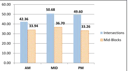
The mean TBST values by time of the day by bus stop location-type are presented in Figure 4. From the figure, it can be observed that the mean TBST values of buses at midblock bus stops are lower than the mean TBST of buses at bus stops located at intersections for the observed periods. The peak TBSTs for both bus stop location-types were observed during midday.
21 Results 42.36 50.68 49.60 33.94 36.70 33.26 0.00 10.00 20.00 30.00 40.00 50.00 60.00 AM MID PM Intersections Mid-Blocks
Figure 4. Mean TBST Values by Time of Day by Bus Stop Location-type
REGRESSION ANALYSIS
Regression models were developed by bus stop location-type and by time of the day using the data obtained for sixty bus stops. The TBST model was determined as follows:
𝑇𝑇𝑇𝑇𝑇𝑇𝑇𝑇=𝑓𝑓(𝐷𝐷𝑇𝑇,𝑃𝑃𝑏𝑏,𝑃𝑃𝑎𝑎,𝑃𝑃𝑘𝑘,𝐿𝐿𝑛𝑛,𝑇𝑇𝑝𝑝)
while the DT model was determined based on 𝐷𝐷𝐷𝐷=𝑓𝑓( 𝑃𝑃𝑏𝑏,𝑃𝑃𝑎𝑎,𝑃𝑃𝑘𝑘,𝐿𝐿𝑛𝑛,𝐵𝐵𝑝𝑝)
with independent variables previously defined.
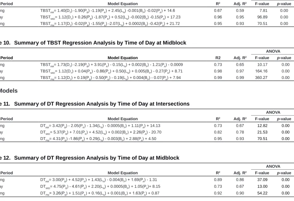
The adequacy and significance of the regression models were tested at a significance level of 5%. Summaries of the regression analyses are presented in Table 9 through Table 12. The detailed results of the regression analyses are presented in Appendix 4.
The results shown in Table 9 and Table 10 for the TBST models indicate that the models could explain relatively high percentages of the variations in the data, based on the R2 values (67-96%). For both bus stop types, the morning period shows a lower explanatory power compared to the models for the remaining two. In addition, the p-values for the regression models’ F-statistics were determined to be less than 0.05, indicating that the coefficients are not equal to zero at 5% level of significance.
The results shown in Table 11 and Table 12 for the DT models also indicate that the models could explain relatively high percentages of the variations in the data, based on the R2 values (73-95%). The highest R2 values for the DT models were observed during the p.m. periods for both bus stop types. Further, the p-values for the regression models’ F-statistics were determined to be less than 0.05, indicating that the coefficients are not equal to zero at 5% level of significance.
22 Results
The p-values of t-statistics of the models’ coefficients (for both bus types and periods) indicate that DT was the most significant independent variable that predicts the TBST. The remaining coefficients all indicated p > 0.05.
Mineta National
T
ransit Research Consortium
23
Results
TBST Models
Table 9. Summary of TBST Regression Analysis by Time of Day at Intersections
Time Period Model Equation R2 Adj. R2
ANOVA F-value p-value
Morning TBSTAM= 1.40(DT) -1.90(PB) -1.19(PK) + 2.45(LN) -0.001(BP) -0.02(PA) + 14.6 0.67 0.59 7.81 0.00
Midday TBSTMID= 1.12(DT) + 0.26(PB) -1.87(PK) + 0.52(LN) -0.002(BP) -0.15(PA) + 17.23 0.96 0.95 96.89 0.00
Evening TBSTPM= 1.17(DT) -0.02(PB) -1.55(PK) -2.07(LN) + 0.0002(BP) -0.42(PA) + 21.72 0.95 0.93 70.51 0.00
Table 10. Summary of TBST Regression Analysis by Time of Day at Midblock
Time Period Model Equation R2 Adj. R2
ANOVA F-value p-value Morning TBSTAM= 1.73(DT) -2.19(PB) + 3.91(PK) - 0.15(LN) + 0.002(BP) - 1.21(PA) - 0.0009 0.73 0.65 10.17 0.00 Midday TBSTMID= 1.12(DT) + 0.04(PB) - 0.86(PK) + 0.50(LN) + 0.005(BP) - 0.27(PA) + 8.71 0.98 0.97 164.16 0.00 Evening TBSTPM= 1.12(DT) + 0.19(PB) - 0.50(PK) - 0.19(LN) + 0.004(BP) - 0.07(PA) + 7.94 0.99 0.99 360.27 0.00 DT Models
Table 11. Summary of DT Regression Analysis by Time of Day at Intersections
Time Period Model Equation R2 Adj. R2
ANOVA F-value p-value
Morning DTAM= 3.42(PB) - 2.05(PK) - 1.34(LN) - 0.0005(BP) + 1.11(PA) + 14.13 0.73 0.67 12.82 0.00
Midday DTMID= 5.37(PB) + 7.01(PK) + 4.52(LN) + 0.002(BP) + 2.26(PA) - 20.70 0.82 0.78 21.53 0.00
Evening DTPM= 4.31(PB) -1.86(PK) + 0.29(LN) - 0.003(BP) + 2.88(PA) + 4.50 0.95 0.93 70.51 0.00
Table 12. Summary of DT Regression Analysis by Time of Day at Midblock
Time Period Model Equation R2 Adj. R2
ANOVA F-value p-value
Morning DTAM= 3.00(PB) + 4.52(PK) + 1.43(LN) - 0.004(BP) + 1.69(PA) - 1.31 0.89 0.86 37.09 0.00
Midday DTMID= 4.75(PB) - 4.61(PK) + 2.20(LN) + 0.0005(BP) + 1.05(PA)+ 8.15 0.73 0.67 13.00 0.00
24 Results
MODEL VALIDATION
Residual and Normal Probability Plots
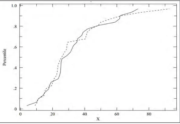
For a valid regression model, the residuals would approximate the random errors that establish the relationship between the explanatory variables and the response variables. Therefore, if the residuals appear to behave randomly, it suggests that the model fits the data well. The normal probability plots were also used to determine the validity of the models. If all the data points fall near the line, an assumption of normality is reasonable, otherwise, the points will curve away from the line. Figures 5 and 6 are the respective residual plots and normal probability plots for the regression model for bus stops located at intersections by midday. The remaining plots by bus stop type and time period are presented in Appendix 4.
For all the models by bus stop type and time period, the residual plots showed evenly distributed random plots about the zero line, confirming that the models fit the data sets well. Also, the normal probability plots show a line along the points, thus an assumption of normality would be reasonable for the data sets. Thus, from the figures, it can be concluded that the models adequately predict TBST and DT.
120 100 80 60 40 20 10 5 0 -5 -10 Fitted Value Re si du al Versus Fits (response is TBST)