Chapter 11
Decision Making in Finance:
Time Value of Money, Cost of Capital and Dividend Policy
Babita Goyal
Key words: Present value of a flow, future value of a flow, annuity, doubling period, compounding, effective interest rate, nominal interest rate, return, investment, cost of debt, cost of equity, cost of preference stock, weighted cost of capital marginal cost of capital
Suggested readings:
1. Chandra P. (1970), Appraisal Implementation, Tata-McGraw Hill Publishing Company Limited, New Delhi.
2. Hampton J.J. (1992), Financial Decision Making (4th edition), Prentice hall of India Private Limited
3. Khan M.Y. and Jain P.K. (2004), Financial Management (4th edition), Tata-McGraw Hill Publishing Company Limited.
4. Gupta P.K. and Mohan M. (1987), Operations Research and Statistical Analysis, Sultan Chand and Sons, Delhi.
11.1 Introduction
The major objective of the financial decision-making is wealth maximization. In wealth maximization, the timings at which benefits are received play an important role. A financial decision spreads over time horizon, i.e., it ventures into the future. For example, a new piece of equipment installed today, will be useful for many years (useful life of the equipment) to come. However, the payment for this equipment may also be spread over many years to come. Then a financial decision is to be made on the basis of the cash outflows (i.e. the payments) and the cash inflows (i.e., the benefits) associated with the decision. In such situations, in order to facilitate effective and valid comparisons, it is necessary that the cash flows during different time periods have the same monetary value. From this requirement originates the concept of “time value of money”. Money has time value. This simply means that the value of money is different at different time periods. A rupee today is more valuable than a rupee one year from now. Worth of money changes due to the following reasons.
(i) In general, individuals prefer present consumption to future consumption, as future is uncertain.
(ii) Capital can be invested to generate positive returns, so if r is the annual rate of return, then one rupee invested today would yield Rs. (1+r) one year hence, so Rs. (1+r) after one year will have the same worth as one rupee today.
So, if we are interested in cash flows occurring at various time points, as is the case with most of the financial problems, we have to consider explicitly the time value of money.
11.2 Time value of money
In order to understand the concept of the time value of money, we define the following terms.
(i) Future value of a single flow Suppose that we want to invest an amount P for n years at a rate of interest of i %. Then the future value of amount P is defined as
(1 )n
S = P +i (11.1)
Where S is the future value after n years.
The factor (1+i)nis called the compounding factor or the future value interest factor
.
,(FVIFi n) If the interest is compounded continuously, then the future value of the flow is given by
in
S = P e
(ii) Present value of a single flow For a single flow
(1 )n S P i = + (11.2) The factor 1
(1+i)n is called the discounting factor or the present value interest factor . Tables
are available to calculate for different values of n and i.
,
(PVIFi n)
,
i n
PVIF
If the interest is compounded continuously, then the present value of the flow is given by
in
P = Se−
Doubling period Doubling period of an investment is the time needed to double that investment. Using equation (6.1), we calculate the doubling period of investment P as follows:
2 (1 ) 2 (1 )
or, log 2 log (1 ) log 2 log (1 ) 0.301 log (1 ) n n P P i i n i n i i = + ⇒ = + = + ⇒ = + = +
(iii) Future value of an annuity An annuity is a series of periodic cash flows (payments or receipts) of equal amounts. The cash flows may occur at the beginning or at the end of a period. If the cash flows are occurring at the beginning of the period, the annuity is called an annuity due and if the cash flows are occurring at the end of the period, the annuity is called a regular or deferred annuity.
We define the future value of an annuity as the amount received in future when an annuity is invested at a given rate of interest. Mathematically,
1 2
(1 ) (1 ) ... (1 ) 1
where, Future value of a regular annuity which has a duration of period; n n n n n S R i R i R i R i S n − − = + + + + + ⎡ + − ⎤ = ⎢ ⎥ ⎣ ⎦ =
Constant periodic flow; Interest rate per period; and Duration of the annuity.
R i n = = = The factor (1 ) 1 n i i ⎡ + − ⎢ ⎣ ⎦ ⎤
⎥ is called the future value interest factor for an annuity ). Tables are available to calculate for different values of n and i.
,
(FVIFAi n ,
i n
FPVIF
If the interest is compounded continuously, then the future value of the annuity is given by
1 1 in n i e S R e ⎡ − ⎤ = ⎢ ⎥ − ⎣ ⎦
(iv) Sinking fund factor Reciprocal of , the sinking fund factor is the discounting factor of a future flow. So
, (FVIFAi n) (1 ) 1 n n i R S i ⎡ ⎤ = ⎢ ⎥ + − ⎣ ⎦ and (1 )n 1 i i ⎡ ⎢ + − ⎣ ⎦ ⎤
(v) Present value of an annuity Present value of an annuity is its present worth discounted at a rate equal to the rate of interest. Mathematically,
2 1 1 1 1 ... 1 1 1 (1 ) 1 (1 ) n n n n P R R R i i i i R i i − ⎡ ⎤ ⎡ ⎤ ⎡ ⎤ = ⎢ ⎥+ ⎢ ⎥ + + ⎢ ⎥ + + + ⎣ ⎦ ⎣ ⎦ ⎣ ⎦ ⎡ + − ⎤ = ⎢ ⎥ + ⎣ ⎦
where, Present value of a regular annuity which has a duration of period; Constant periodic flow;
Interest (discount) rate per period; and n P n R i n = = =
= Duration of the annuity.
The factor (1 ) 1 (1 ) n n i i i ⎡ + − ⎤ ⎢ + ⎣ ⎦⎥ ) ,
is the present value interest factor for annuity (PVIFAi n,
.
It can be seen that, = ,
i n i n i n
PVIFA FVIFA × PVIF
Tables are available to calculate PVIFAi n, for different values of n and i.
Example 1: The payment to a 10 period annuity of Rs. 5,000 will begin seven years from now. What is the present value of the annuity at a discount rate of 12%?
Sol: The value of this annuity one year prior to its maturity, i.e., six years from now, will be
12,10
Rs.5, 000 = 5, 000 5.650 (from tables) = Rs. 28, 250
PVIFA
× ×
Present value of this amount is
12,6
Rs. 28, 250 = 28, 250 .507 (from tables) = Rs. 14, 323
PVIF
(vi) Capital recovery amount Capital recovery amount, R, is that amount which can be withdrawn periodically for a certain length of time in response to a certain investment today. Mathematically (1 ) 1 (1 ) (1 ) (1 ) 1 n n n n n n i P R i i i i R P i ⎡ + − ⎤ = ⎢ ⎥ + ⎣ ⎦ ⎡ + ⎤ ⇒ = ⎢ ⎥ + − ⎣ ⎦ The factor (1 ) (1 ) 1 n n i i i ⎡ + ⎤ ⎢ + −
⎣ ⎦⎥ is called the capital recovery factor.
(vii) Present value of an uneven series Till now, we have derived various expressions assuming that cash flows associated with an annuity are equal in amount. However, this situation may not always be true and various cash flows associated with an annuity are unequal in amount. For example, the dividend stream of an equity is consists of unequal payments. The present value of an uneven series is, then, calculated by considering all the cash flows occurring at various time points:
2 1 2 1 1 1 1 ... 1 1 1 (1 )
where, Present value of a cash flow stream which has a dura
n n n n t t t n PV R R R i i i R i PV = ⎡ ⎤ ⎡ ⎤ ⎡ ⎤ = ⎢ ⎥+ ⎢ ⎥ + + ⎢ ⎥ + + + ⎣ ⎦ ⎣ ⎦ ⎣ ⎦ = + =
∑
tion of period; Cash flow occurring at the end of the period ;Interest (discount) rate per period; and Duration of the cash flow stream.
t n R t i n = = =
(viii) Shorter compounding periods Sometimes the interest is not compounded annually but for shorter periods. In this case the future value of the annuity can be calculated as follows:
1 mn i S P m ⎛ ⎞ = ⎜ + ⎟ ⎝ ⎠
where, Future value after years; Present amount;
Nominal interest rate per year;
Number of times compounding is done during a year; and n S n P i m = = = =
n = Duration of the compounding.
The difference of the principals of the annual compounding and the shorter period compounding represents the interest on annual interest.
Effective versus nominal rate Consider the following offer of a company.
AEO Ltd. is offering 12% interest semi-annually on the investments made to the company. A person wants to invest a sum of Rs. 10,000. Calculate the amount, which he will receive after one year.
(a) If the compounding is done semi-annually:
(i) First six months:
Principal at the beginning = Rs.10,000.00 0.12 Interest of six months = Rs. 10,000
2 = Rs. 600.
×
Principal at the end = Rs.10,000.00 + Rs. 600. = Rs.10,600.00
(ii) Second six months:
Principal at the beginning = Rs.10,600.00 0.12 Interest of six months = Rs. 10,600
2 = Rs. 636.
Principal at the end = Rs.10,600.00 + Rs. 636.
×
(b) If the compounding is done annually:
Principal at the beginning = Rs.10,000.00 Interest of six months = Rs. 10,000 0.12 = Rs. 1200.
Principal at the end = Rs.10,000.00 + Rs. 1200.
×
= Rs.11,200.00
The difference between the two principals, i.e., Rs. 36 is the interest on interest of the first six months for the second six months. Thus in the case of semi-annual compounding the principal is growing effectively at a rate of 12.36% annually. Now, we can differentiate between effective and nominal rates of interest:
Nominal rate of interest is that rate which is offered at an annual basis, irrespective of the number and size of the compounding periods.
Effective rate of interest is that rate at which the principal is actually growing annually if the size of the compounding period is less than the size of the period for nominal rate. In fact this is the rate under annual compounding which will let the principal grow at the same rate at which shorter period compounding is being done.
There exists a mathematical relationship between effective and nominal rates of interest:
( ) 1 1 m m i i m ⎛ ⎞ = ⎜ + ⎟ − ⎝ ⎠ ( )
where, Effective interest rate per year; Nominal interest rate per year;and
Number of times compounding is done during a year.
m i i m = = =
( ) 1 1 1 m m i d i d m = + ⎛ ⎞ = − −⎜ ⎟ ⎝ ⎠
(m) Nominal discounting rate per year
d =
11.3 Applications of present value and future value techniques
There are some situations in real life where we have to compare the cash flows at two different time points. In such situations these techniques can be used effectively to make meaningful comparisons.
(1) An annual saving of a certain sum may be required to generate a fund which would be needed
sometime in future, e.g., to repay an existing liability or to replace a piece of equipment. Then the fund manager is interested in knowing the size of the annuity to generate the required fund.
Example 2: A company has sold 7.5% bonds that will mature after 8 years from today. Now the company plans to create a fund for repayment of bonds in which a fixed amount is to be deposited (at the end of) each year. If the funds are expected to earn 7% annual interest, find the amount of the annuity needed to accumulate a sum of Rs. 10, 00,000 at the end of 8 years.
Sol: In this case we have to find the size of a 5-year annuity whose future value is Rs. 10, 00,000
7,8 10.26
10, 00, 000
Size of the annuity = = Rs. 96252. 10.26
FVIFA =
⇒
(2) When the loan, which has been borrowed today, is to be repaid in future, the fund manager is
interested in knowing the size of the annuity.
Example 3: A company has installed a machine worth Rs. 15, 00,000.the amount has to be repaid in 5 equal installments at an interest rate of 12 %. Find the size of the annuity.
Sol: In this case we have to find the size of a 5-year annuity whose present value is Rs. 15,00,000.
12,5 3.605
15, 00, 000
Size of the annuity = = Rs. 4,16, 089. 3.605
PVIFA =
⇒
(3) The market price of shares and securities are significantly affected by the dividends paid by
the company offering them. If the growth rate of dividends is higher than the prevailing interest rate or the growth rate of other securities, the market price of shares will be high. An investor may be interested in determining the growth rate of dividends that he is receiving.
Example 4: Given below are the dividends received by Mohan from a certain infrastructure company: Table 11.1 Year Dividends (Rs.) 1 25.00 2 28.35 3 32.80 4 35.50 5 38.00 6 40.27
The rate of return on other similar securities is 8%. Mohan wants to know whether or not should he dispose off his stock. What should he do?
Sol: Since the dividends are received at the end of the period (year), so the above table reveals that the dividends have grown from Rs. 25 to Rs. 40.27 in five years’ time. Thus
5 5 40.27 25.00(1 ) 40.27 (1 ) 1.611 25.00
10% (From compounding tables)
i i i = + ⇒ + = = ⇒ =
Since Mohan is earning dividend, which has a growth rate higher than the growth rate of similar securities in the market, he should not sell his stock.
Example 5: Calculate the value five years from now of a deposit of Rs. 20,000 made today at the rate of interest (i) 8%, (ii) 10%, (iii) 12%, and (iv) 15%.
Sol: 5 (1 ) n 20000(1 ) S = P +i = +i (i) i = 0.08 (1 ) 20000(1.360) if 4; 20000(1.587) if 6 1.360 1.587 20000 2 20000 1.473 . 29460 n S P i n n S Rs = + = = = = + ⎛ ⎞ ⇒ ≈ ⎜ ⎟ ⎝ ⎠ = × = (ii) i = 0.10 1.464 1.772 20000 2 20000 1.618 . 32360 S Rs + ⎛ ⎞ ≈ ⎜ ⎟ ⎝ ⎠ = × = (iii) i = 0.12 1.574 1.974 20000 2 20000 1.774 . 35400 S Rs + ⎛ ⎞ ≈ ⎜ ⎟ ⎝ ⎠ = × = (iv) i = 0.15 20000 2.011 . 40200 S Rs ≈ × =
Example 6: A retiring person has been offered two alternatives, between which he has to make a choice: (a) An annual pension of Rs.30, 000 as long as he lives; and (b) a lump sum amount of Rs. 2, 00,000. If the expected life of that person is 15 years more after retirement and that prevailing rate of interest is 15%, which option is more lucrative?
Sol: (a)
15
(1 0.15) 1
Future value of the annuity after 15 years = 30, 000
15 = 30, 000 47.50 ⎡ + − ⎤ ⎢ ⎥ ⎣ ⎦ × = Rs.14, 25, 000 (b) 15
Future value of the single after 15 years = 2, 00, 000(1 0.15) = 2, 00, 000 8.137
+ × = Rs.16, 27, 400
Second option is a better one.
Example 7: What will be the size of the annuity if Rs. 1,00,000 deposited in a bank at an interest rate of 10% reduces to zero in 30 years?
Sol: 30 30 (1 ) (1 ) 1 .10(1 .10) 1, 00, 000 (1 .10) 1 1, 00, 000 9.427 Rs. 10, 608 n n n i i R P i ⎡ + ⎤ = ⎢ ⎥ + − ⎣ ⎦ ⎡ + ⎤ = ⎢ ⎥ + − ⎣ ⎦ = ≈
Example 8: A firm has installed a new machine at a down payment of Rs. 2,50,000 and will pay Rs. 2,00,000 and Rs. 1,00,000 respectively for first two years and rest will be paid in 10 equal installments of Rs. 75,000. If the interest is charged at rate of 12% per annum, what is the present worth of the machine?
Sol: Since the cash flows are uneven, we calculate the present worth of each of the outflow:
(i)
Present worth of Rs. 2, 00, 000 due in one year = 2, 00, 000 0.893 = Rs. 1, 78, 600
×
(ii)
Present worth of Rs. 1, 00, 000 due in two years = 1, 00, 000 0.797 = Rs. 79, 700
×
(iii)
Present worth of an annuity of size Rs. 75, 000 at the beginning of year 3 = 75, 000 0.4.968
×
= Rs. 3, 72, 600 Present worth of a single flow at the beginning of year 3
= Rs. 3, 72, 600 × 0.797 = Rs. 2, 96, 962.2
Hence the total cost of the machine is
= Rs. 2, 50, 000 Rs. 1, 78, 600 Rs. 79700 Rs. 2, 96, 962.2 Rs. 8, 05, 262.2
+ + +
=
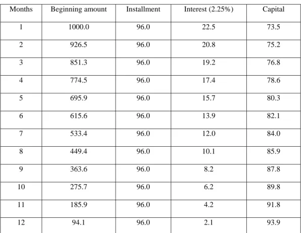
Example 9: A lease contract requires payment of Rs. 96 per thousand per month at the end of every month over a period of 12 months. Develop a repayment schedule.
Sol: The implied effective rate of interest is
,12 ,12 Rs. 96 1000 1, 000 = = 10.4167 96 m m i i PVIFA PVIFA × = ⇒ From tables 2,12 3,12 10.575 9.954 PVIFA PVIFA = =
10.4167 10.575 = 0.02 0.01 9.954 10.575 0.1583 = 0.02 0.01 0.621 m i ⎛ − ⎞ ⇒ +⎜ × ⎟ − ⎝ ⎠ ⎛ ⎞ +⎜ × ⎟ ⎝ ⎠ = 0.0225 = 2.25% Effective rate of annual interest
(
)
121.0225 1 1 0.306 30.6%
= − − =
= Nominal rate of interest = 12 0.0225 = 27%×
Table 11.2: Loan repayment schedule (Rs.)
Months Beginning amount Installment Interest (2.25%) Capital
1 1000.0 96.0 22.5 73.5 2 926.5 96.0 20.8 75.2 3 851.3 96.0 19.2 76.8 4 774.5 96.0 17.4 78.6 5 695.9 96.0 15.7 80.3 6 615.6 96.0 13.9 82.1 7 533.4 96.0 12.0 84.0 8 449.4 96.0 10.1 85.9 9 363.6 96.0 8.2 87.8 10 275.7 96.0 6.2 89.8 11 185.9 96.0 4.2 91.8 12 94.1 96.0 2.1 93.9
11.4 Cost of capital
The cost of capital of a firm is the minimum rate that the firm must earn on its investmentsin order to satisfy the expectations of its investors who provide the funds to the firm. The cost of capital is used for (i) evaluating the net present value of the investments; and (ii) determining the attractiveness of the internal rate of return.
If a firm's rate of return on its investments is more than its cost of capital, it results in enhancement of the wealth of the (equity) shareholders. This is due to the fact that in this case the rate of return earned on the equity capital after meeting all other costs of financing, is more than the rate of return required by the investors. Hence the wealth of the shareholders will increase.
For example, consider a firm whose cost of equity and debt are respectively 14% and 6%and the firm employs equity and debt in equal proportions. The cost of capital for the firm, which is the weighted average cost of capital, is 10%. If the firm invests Rs. 50 lakhs on a project, which is expected to earn 18% rate of return, then the rate of return on equity funds will be given by
Total return on the project - Interest on debt Rate of return on equity =
Equity funds 50 0.18 25 0.06 = 25 = 0.3 = 30 × − × %
This rate of return is greater than that required by the investors (14%). Therefore the market value of the equity capital will increase and hence the wealth of the equity stockholders.
A firm's cost of capital is the weighted average of the cost of various sources of finance used by it. Hence to calculate the cost of capital for the firm, we need to know
(i) The cost of different sources of finance; and
(ii) The proportions of different sources of finance in the capital structure of the firm.
(i) The risk characterizing new investments proposals under consideration is same as the risk characterizing the existing investments of the firm, and the adoption of the new proposals will not change the risk structure of the firm.
(ii) The capital structure of the firm will not be affected by the new investments, and the firm will continue to pursue the same policies; and
(iii) Each new investment is deemed to be financed from a pool of funds in which the various
sources of long-term financing are present in the proportions in which they are found 9n the capital structure of the firm.
11.5 Cost of different sources of finance
The total cost of a source of finance may be deemed to be consisting of two components: (a) Explicit cost; and (b) Hidden cost.
(a) Explicit cost The explicit cost is the rate of discount, which equates the present value of the expected payment to that source of finance with net funds received from that source of finance. Mathematically, it is the value of k in
1 ; (1 ) t t t C P k ∞ = = +
∑
whereNet funds received from the source; and
t Expected payment to the source at the end of the period .
P
C t
= =
For calculating the cost of capital of the firm, we work with the explicit cost of different sources of finance.
(b) Hidden cost hidden cost of a source of finance is the increase in the explicit cost of other sources of finance as a result of employment of the source of finance being considered.
For example, consider a firm, which presently employs Rs. 50 lakh of equity funds at a cost of 12%. Now the firm plans to raise additional funds of Rs. 100 lakh by issuing debentures having an explicit
cost of 6%. However the cost of existing equity capital increases from 12% to 14% as a result of employing debenture capital. This increase is on account of perceiving greater risk in the company due to debenture capital. Hence equity shareholders demand greater return. This increase in the equity cost, as a result of employing debt capital, is a hidden cost of debt. However, hidden costs are not treated separately and these are reflected finally in the explicit cost.
Another cost is the implicit cost, which is the rate of return earned on the best alternative possible investment on which the funds of a source may be employed.
(c) Cost of debt The explicit cost of debt is the discount rate which equates the present value of post-tax interest payment and principal repayments with the net proceeds of debt issue. Mathematically, the cost of debt is the value of kd in the equation
1
(1 )
;
(1 ) (1 )
where
Net funds received from the debt;
t n t d d C T F P k k P ∞ = − = + + + =
∑
Annual debt interest payment ; Tax rate;
Redemption price, which is generally the face value of the debenture;and Maturity period of the debenture.
C T F n = = = =
The debt interest is a tax-deductible expense, that is why C is multiplied by (1-T). In other words, C is in pre-tax terms and C (1-T) is in post-tax terms.
1 1 (1 ) (1 ) (1 ) (1 ) 1 (1 ) (1 ) n t n t d d n d n d d C T F P k k k F C T k k = + − = + + + ⎛ + − ⎞ = − ⎜ ⎟ + + ⎝ ⎠
∑
and(1 ) 2 d F P C T n k F P − − + +
If the difference between F and P is amortized evenly over the duration of debt financing then
(1 ) (1 ) 2 d F P C T T n k F P − − + − +
Perpetual debt If the maturity period of the debt capital is infinite, the debt is called perpetual debt. For this debt, the cost of capital (debt) is the value of kd in the equation
1 (1 ) (1 ) (1 ) (1 ) t t d d d C T P k C T k C T k P ∞ = − = + − = − ⇒ =
∑
Term loans Term loans are the debts raised from the financial institutions or banks, which are repayable normally within 8 to 11 years in equal installments which are either yearly or half yearly after an initial grace period of one to four years. The post-tax cost of a term loan is
Interest rate(1-tax-rate)
If Idstands for total interest on debt and Md is the total market value of debt, then
; d d d d d d I k M I M k = =
Example 10: A firm issues 14% debentures having face value Rs. 100. The net amount realized per debenture is Rs. 96, and the debentures are redeemable after 12 years. The tax rate is 40%. What is the cost of debentures to the firm?
Sol: (1 ) 2 d F P F P C T n k − − + + 100 96 14(1 0.40) 8.4+0.5 8 = 0.09 100 96 98 2 − − + +
Thus the cost of debentures to the firm is approximately 9%.
Example 11: A firm is planning to raise capital through issue of 15% debentures at face value of s. 200. The cost of issue works out to be 2%. The debentures are repayable after seven years. The firm has a tax rate of 40%. If the difference between the par value and the net amount realized can be
ly R
amortized even over the life of the debentures, what is the cost of debt to the firm?
Sol: Net amount realized per debenture =
98 200 Rs. 196 100 × = (1 ) (1 ) 2 200 196 14(1 0.4) (1 0.4) 7 200 196 2 2.4 8.4+ 7 0.044 4.4% 198 d F P C T T n k F P − − + − ⇒ + − − + − = + = = =
(d) Cost of preference capital
Preference capital is that source nance, which carries a fixed rate of dividend. Though this
dividend is payable at the discretion he board of directors, generally it is paid regularly. The cost of preference, which is perpetual, is the value ofkp in the equation
of fi of t
1 (1 ) where t p d D D P k k ∞ = = = +
∑
Net amount relized per preference share; and Preference dividend per share payable annually.
t p P D D k P = = ⇒ =
Redeemable preference stock The preference stock which is not perpetual, i.e., redeemable after
n years, is called the redeemable preference stock. The cost of such stock is the value of kp in the
equation 1 (1 ) (1 ) where t n t p p P k k = = +
The redemption price; and Maturity period. n D F F n + + = = Then,
∑
2 p F P D n k F P − + +If the difference between F and P is amortized evenly over the duration of capital financing and the tax rate for the firm is T, then
1 (1 )t (1 )n t p p P k k = ( ) n F P T D F n − + = + + +
∑
(1 ) 2 p F P D T n k F P − − − ⇒ +Example 12: A firm is issuing preference shares at a dividend rate of 12%. The preference capital is repayable in two equal installments at the end of the 10th and th 11th year respectively. The amount realized per preference share is Rs. 97. What is the cost of the preference capital?
Sol: 10 11 2 D k F P 1 1 12 (100 97) 10 11 197 2 p F−P F−P + + + ⎛ ⎞ + − ⎜ + ⎟ ⎝ ⎠ = 21 12 3 110 0.1269 12.69% 197 2 ⎛ ⎞ + ⎜⎝ ⎟⎠ = = =
(e) Cost of equity capital
The cost of equity capital is the minimum rate required on the net equity funds raise n order to leave the market price of the equity stock unaffected.
To calculate the cost of equity capital, we must know the rate of return required by the equity
d by the equity stockholders is difficult to know. Several approaches have been suggested to stimate this rate.
d i
stockholders, which is then adjusted for the floatation costs when the firm issues the additional equity stock.
Rate of return required by the equity stockholders The dividend stream receivable by the equity stock holders is not governed by any contract or fixed rules. Hence measuring the rate of return require
e
(i) Dividend forecast approach The value of an equity stock is equal to the sum of the present value of dividends associated with it, i.e.,
1
;
(1 )
where
P = Price per share of equity stock;
Expected dividend at the end of the period ; and Rate of return required by the equity stock holders.
t t t e t e D P k D t k ∞ = = + = =
∑
If the future dividend stream, as expected by the equity stock holders can be forecasted, then given the current market price per equity share, the rate of return can be calculated.
If the dividend is expected to be constant annually then
e
D k
P
If the equity stockholders expect the dividend to grow annually at a rate of g % forever, then keis given
by the expression 2 1 1(1 ) 1(1 ) D D g D g ... P = + + + + + + 1 1 2 3 1 (1 ) ... 1 (1 ) (1 ) (1 ) 1 (1 ) 1 1 t t e e e e e e D g k k k k k g k − + + + + + + + + = + − + D 1 1 1
1 since if , prices will tend to
1 e e e e D g g k k g k D k g P ⎛ + ⎞ = ⎜ < > ⎟ − ⎝ + ⎠ ⇒ = + ∞
Thus the cost of equity capital is equal to the dividend yield plus the annual growth rate of dividend.
Example 13: The market price per share of a company is Rs. 20.00 and the dividend expected one year from now is Rs. 1.25. The expected rate of dividend growth is 6%. What is the cost of equity capital to the company?
Sol: 1 1.25 0.06 20 0.1225 12.25% = + = = e k g P D = + If D/P ratio is 100%, then g = 0
1 1
1
1
; is the number of outstanding equity shares and
is the earnings in period 1.
; e d e D E k P P E N N PN E EBIT I M M = = = −
= e is the total market value of equity
; is the net income available to shareholders.
e e e NI NI M NI M k = ⇒ =
When the expected growth rate of dividend varies over time, this variation has to be taken into account. Suppose that the expected growth rate is g1 for n1 years, g2 for n2 years and g3 forever after that, and then the equation for ke is
1 2 1 1 2 1 1 1 2 3 1 1 1 1 1 (1 ) (1 ) (1 ) (1 ) (1 ) (1 ) t t t n n n n n t n t t e t e t e D g D g D g P k k k − ∞ + + + = = = + + + = + + + + +
∑
∑
∑
n n2+ts Rs. 20 per share, which is expected to grow at a rate of 10% per share e years. Thereafter the growth of the dividend is expected to decline to 8% where it will stay forever. What is the cost of equity to the company?
.
Sol: The cost f equity to the company is the value of kein the equation
Example 14: The market price per share of a company is Rs. 150 at present. The dividend expected one year from now i
for fiv o 1 4 5 5 1 1 1 4 5 1 20(1 0.10) 20(1 0.10) (1 0.08) 150 (1 ) (1 ) 20(1.10) 20(1.10) (1.08) 1.08 (1 ) t t t t t e t e t t t t e k k k − ∞ + = = − = + + + 5 0.08 (1 ke) ke = + + + ⎜ − ⎟ + ⎝ ⎠ ⎛ ⎞ = + +
∑
∑
∑
(ii) Realized yield approach According to this approach, the yield realized by equity shareholders historically is regarded as a proxy for the rate of return required by them. The yield on an equity stock for the year is given by
d of the period ; and
pr er share at the end of the period 1,i.e. at the beginning ofthe period .
t t P t P− t t = = − where
Yield for year ;
Dividend at the end of the period payable at the end of the period;
t t Y t D t = = 1
price per share at the en ice p 1 t t t D P P− +
is called the wealth rate.
The yield for the n-year period is
1 1 1 1 n n t t t t D P P = − ⎛ + ⎞ − ⎜ ⎟ ⎝ ⎠
∏
The basic assumptions of this approach are
(i) The y stor and the expectations of the investor are similar; and
(ii) The investors’ expectations in future will be similar to those in the past.
Example 15: The dividend per share and the price per share data of an equity stock are given
Year Dividend per share (Rs.) (D) Price per share (Rs.) (Pi)
ield earned by the inve
below Table 11.3 i 1 3 4 6 1.00 1.25 1.50 1.75 10.00 11.00 11.50 12.00 2 1.15 10.5 5 1.50 10.75 1 t t 1; t t D P Y P− + = −
Obtain the y for the five-year period k.
Sol: We calculate the wealth ratio as follows
able 11.4
Year Di (Rs.) ) (Rs.) (Pi+1) (Rs.)
Wi =
ield on this stoc
T (Pi 1 t t t D P P− + 1 2 3 4 5 1.00 1.15 1.25 1.50 0.00 10.50 11.00 0.75 10.50 11.00 11.50 10.75 12.00 1.15 1.16 1.16 1.07 1.26 1 1.50 11.50 1 6 1.75 12.00 - 5 1 1 5 5 1 56 1.15 0.156 i i i i w w Y = = = ⎛ ⎞ ⎜ ⎟ ⎝ ⎠ = −
∏
∏
2.06 1.1 = 6 1=Thus th return on the st s 15.6%.
However, the assumptions of this approach, particularly the second assumption is somewhat unrealistic. The investors’ expectations change with the anticipated change in rate of inflation and subsequently change in the interest rate structure. Thus if historical return (yield) is to be used as a proxy for the future rate of return, appropriate caution must be taken. However, the historical figure may
1.6 Capital asset pricing model (CAPM)
investors eliminate the unsystematic component of the risk by diversifying their portfolios efficiently
e ock i
serve as a starting point to obtain estimates of the future.
1
As we have already seen, CAPM can be used for pricing of assets and portfolios. Also we have used this model for the determination of required rate of return. This method is based on the assumption that
and are needed to be compensated for the systematic component of the risk, which is reflected in the beta coefficient. However due to market imperfections, unsystematic component of the risk may creep to the model for which the investor should be appropriately compensated. But this feature is missing
he
(i) Earning price ratio approach in
from t model.
Another limitation of the model lies in the instability of the beta. This makes the use of historical value of beta somewhat unsuitable. In spite of this limitation this model is used widely in making financial decisions.
According to this approach, the rate of return required by the equity investors is
where
Et = Expected earnings per share for the next year
Current earnings per share(1+growth rate of earnings per share) et price per share.
t e E k P = =
(i) The earnings per share are expected to remain constant and the dividend payout ration is
100%;
The cost of equity capital in this case is the value of ke in the expression
P = Current mark
The approach can be used appropriately when
1 (1 ) ke P ⇒ = t t e e D P k D k D ∞ = = + =
∑
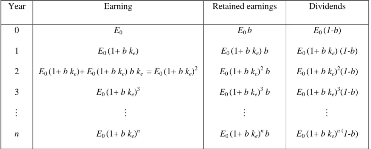
(ii) When the retained earnings are expected to earn a rate of interest equal to the rate of return
As a simple case, let the firm be an all-equity firm. Let the retention rate of the firm is b% in each period which is constant.
Since the reinvested funds earn a return equal to ke %, the earnings, retained earnings and the dividends
are given by the following expressions
Year Earning Retained earnings Dividends
Table 11.5 0 1 2 n E E0 (1+ b ke) E0 (1+ b ke)+ E0 (1+ b ke) b ke = E0 (1+ b ke)2 E0 (1+ b ke)n E b E0 (1+ b ke) b E0 (1+ b ke)2 b E0 (1+ b ke)n b E (1-b) E0 (1+ b ke) (1-b) E0 (1+ b ke)2(1-b) E0 (1+ b ke)n (1-b) 0 0 0 0 (1+ b ke)3 M E0 (1+ b ke)3 b E0 (1+ b ke)3(1-b) 3 M E M M Now, 1 0 1 P = (1 ) (1 ) (1 ) (1 ) t t t e t e t t e D k E bk b k ∞ = = + ∞ + − +
∑
∑
= 0 1 1 (1 )(1 ) (1 ) e e ke e E bk b E k b E k P + − − ⇒ =However both these situations are difficult to meet in practice. As such this method should be used with caution.
(ii) Bond yield plus risk premium approach
According to this approach, the rate of return required by the equity investors is given by
Yield on the long-term bonds of the firm + risk premium.
The approach rests on the assumption that the equity investors have a higher degree of risk than the bondholders and hence their required rate of return should include a risk premium in addition to the
However, there is no sound theoretical basis for defining the risk premium and it is subjective quantity based on operating risk and the risk preference of the firm.
The firm should thus earn k holders of the
rm. However this assertion is true when there is no floatation cost, for example, cost of issuing
funds from its retained earnings.
owever, when a firm raises funds by issuing (additional) equity stock, generally floatation cost is incurred. In this case the net funds realized by the firm are less than what has been contributed by the equity holders. In this case, the firm should earn a rate of return higher than the required rate of return by the equity holders to take care of this additional cost. Mathematically, if the floatation cost is f %, and the required rate of return is ke%, then the firm should be able to earn a rate of return equal to
return earned on the long-term bonds.
Adjustment for the floatation cost
a rate of return equal to the rate required by the equity stoc fi
shares, commission, brokerage etc. This will, thus be true in case when the firm obtains the equity
H
%
e
k
on the net equity fund raised by it.
Weighted average cost of capital 1− f
nce the cost of different sources of finance has been determined, the firm’s overall cost of capital is
a
k =
O
the weighted average cost of different sources of finance. Mathematically,
where
a d d p p r r e e
k = w k +w k +w k +w k
kd = cost of debt; wd = weight of debt; kp = cost of p
ost of additional equity; weight of addit
p r r e w k w w = = = = ional equity.
referrence capital; weight of preferrence capital;
cost of retained earnings; weight of retained earnings;
ke = c
If the only sources of finance are equity and debt (as in case of a new company), then
; is the total value of the firm.
d d e e d e d e d e d e d e d e k w k w k M M k k V V V M M k k M M M M = + = + = + + + d d e e d e d d e M k M k M M I NI M M V + = + + = + = EBIT d d d e d d e e I EBIT I EBIT V k k k M k k V k M V − ⇒ = = + ⎛ ⎞ ⎜ ⎟ ⎝ ⎠ ⇒ = ⎛ ⎞ ⎜ ⎟ ⎝ ⎠ 1 d d d M k k V M V ⎛ ⎞ − ⎜ ⎟ ⎝ ⎠ = ⎛ ⎞ − ⎜⎝ ⎟⎠ ( ) ( ) e d e d d e kM k k M M M k k k M d + − = ⎛ ⎞ = + − ⎜ ⎟ ⎝ ⎠
Example 16: Consid nformation available about the four firms A, B, C and D Table 11.6 Firms EBIT (Rs.) Id(Rs.) ke (%) er the i A B C D 4,00,000 6,00,000 5,00,000 8,00,000 40,000 1,00,000 1,00,000 2,00,000 12 10 20 15
Assuming no taxes and the cost of debt at 10%, calculate the total market value and weighted average cost of capital of each firm.
Sol: Particulars A B C D Table 11.7 4,00,00 0,000 1,00,0 5,00,000 1,00,000 8,00,000 00,000 0 6,0 40,000 00 2, 3,60,000 5,00, 0.1 4,00,000 0.20 00,000 0.15 0.12 000 0 6, 30,00,000 4,00,000 50,00, 10,00,000 20,00,000 10,00,000 ,00,000 20,00,000 000 40 34,00,000 60,00,000 30,00,000 60,00,000 EBIT (Rs.) Less: Interest (Rs.) NI (Rs.) ke Me (Rs.) 0.10 d d I M = (Rs.) V (Rs.) EBIT k V = (%) 11.76 10 16.67 13.33 System of weighting
Assig ghts to different sources of finance is an important aspect in determinati of the
overall cost of capital to the firm as variation is weights would lead to variation in the total cost of
capita l methods have been p or dete of weig scuss of
these thod.
(i) Book value method
In this method, the weights are assigned a ording to the v ues found in the balance sheet of he firm.
The w re the proportion of th e of f fina otal v
g-term) finance of rm.
he book value methods are simple to obtain and are fairly stable since book values are not affected by . At times these may be the only available weights e.g., the market values are ot easily available if the firm is not listed or its shares are not actively traded in the market. However,
.
i) Market value weights
proportion of the market value of the source of finance to the total market alue of finance of the firm. Thus these weights are consistent with the concept of the cost of capital.
hich theses sources are providing funds to undertake present and the future ments. Thus these weights are in actual proportion of the sources of finance that would e sources. However the actual mix of capital needed to finance ture investments may be difficult to obtain.
l. Severa roposed f rmination hts. We di here some
me
cc al t
eights a e book valu the source o nce to the t alue of (lon
the fi
T
the market fluctuations n
the method suffers from a number of drawbacks. First of all, the present values of different sources of finance may not be much related to their book values. Secondly book value weights do not go with the concept of the cost of capital, which is the minimum required rate of return to maintain the market value of the firm
(i
In this method, the weights are assigned according to the market values of the sources of finance of the firm. The weights are the
v
However theses weights may be difficult to obtain if the firm is not listed or its shares are not actively traded in the market. Further the speculative forces working in the market may distort the weights.
(iii) Financing planning weights
In this method of assigning weights, weights are assigned to different sources of finance in the proportions in w
invest
correspond to the market value of thes fu
Example 17: Consider the following data
Capital structure of the firm As on March 31
Table 11.8
st, 2006
Book value (Rs. in crores) Market value (Rs. in crores)
Debentures (8.5% due 2010 -13) 1.00 0.87 Debentures (11% due 2017 -21) 2.23 2.77 1.76 2.77 Long-term loan (10%)
Preference capital (7%, market price per share Rs. 50) Net worth 0.89 8.87 0.45 8.75 Table 11.9 Value (Rs.) Equity details 1998 1999 2000 2001 2002 2003 2004 2005 2006 17.4 13.0 16 13.0 17.7 16.4 21.8 20.3 20.3 20.0 .0 .1 13.1 5.0 13.0 13.0 13.0 13.0 13.0 15 1:12 17.4 13.0 16.1 13.0 13.1 5.0 17.8 14.1 23.6 14.1 22 14 22.0 14.1 31.4 16.3 19.2 14.1 .0 .1 Earnings per share
101.25 Dividend per share
Bonus
Adjusted earnings per share* Adjusted dividend per share*
Market price**
* r bonus declaration in 2001
** Market price is the average of high and low in the month when capital structure has been determined.
The effective tax rate for the company is 57.75%. Calculate the cost of capital for the firm.
Sol: ( x cost of 8.5% debentures due 2010-1
These de interest of n repay ble i ur e in ents
starting arket val r 00 face va f t bent 7
2007. The post tax cost of these debentures is that discount rate which would equate the present value Adjusted fo
i) Post ta 3
bentures carry an rate 8.5% a d are a n fo annual qual stallm
of the post-t tflows (interest and the principal ent) with the market value, i.e., the va
ax cash ou repaym
lue of kdin the expression
(
)
(
)
(
)
(
)
(
)
(
)
(
)
2 3 4 8.5(1 0.5775) 8.5(1 0.5775) 8.5(1 0.5775) 8.5(1 0.5775) + + + 1 1 1 1 4.25(1 0.5775) 25 2.125(1 0.5775) 25 0.065 6.5% d d d d k k k k k − − − − + + + + − + − + ⇒ = = tax 87 = 5 6 7 + + + 1+kd 1+kd 1+kd 6.375(1 0.5775)− +25 d(ii) Post cost of 11% debentures due 2017-21
These debentures are payable in five equal annual installments. The post tax cost of these debentures is the value of kdin the expression
(
)
(
)
(
)
(
)
(
)
(
)
10 13 14 15 6.6(1 0.5775) 20 4.4(1 0.5775) 20 2.2(1 0.5775) 20 + + + 1 1 1 0.07 7% d d d d d d d k k k k − − + − + − + − + − + + + + ⇒ = =(iv) Post tax cost of 10% long-term loan
he cost of capital is given by
11 12 t=1 11(1 0.5775) 11(1 0.5775) 20 8.8(1 0.5775) 20 79 + + 1 k t 1 k 1 k = + + +
∑
rate of interest(1-tax rate) 10(1-0.5775) 4.225%
l
k =
= =
(v) Post tax cost of 7% preference capital
For perpetual preference capital t
Annual dividend 7
= = = 14%
Market price 50
p
(vi) Post-tax cost of equity 1 0 8 where
Actual growth rate of dividends over the period 1998-2006 15 13(1 ) 3% e D k g p g g g = + = ⇒ = + ⇒ = Now, 1 0 15.0 101.25 15 0.03 17.2% 101.25 e D p k = = ⇒ = + Then we have Table 11.10
Source of capital Weight (Market value) Cost of the source
Debentures (8.5%) Debentures (11%) Long-term loan Preference capital Equity 0.87 0.10 8.75= 0.20 0.32 0.05 0.33 0.065 0.07 0.04225 0.14 0.172 Cost of capital 0.09862 = 9.862%
Marginal cost of capital
Till now, we have been assuming that the cost of capital remains the same irrespective of the amount of being raised. However, this is a simplified assumption and usually the cost of capital increases after certain amount. This increase in cost while raising additional funds for the firm is called the marginal 11.7
cost of capital. To illustrate this point consider the following situation when a firm has the following capital structure
Table 11.11
Then the marginal cost of capital, which the cost of capital at the margin is given by
3 2 0.15 0.14 (1 0.40) 5 5 0.45+0.252 5 0.1236 12.36% k = × + × × − = = =
However, at this cost of capital the firm cannot raise unlimited fund. As the requirement for the fund rises, the cost of capital is bound to rise. The capital schedule can have jumps at several points when the cost of capital changes. Let the additional information in the above schedule be as follows
(i) The required return on first 40 lakhs of equity is 15% and on the next 60 lakh is 16%.
(ii) The required return on first 60 lakhs of debt is 14% and on the next 40 lakh is 16%.
What can be the composition of the additional funds? To see this, we can calculate the cost of capital corresponding of different composition of the additional funds
Source of capital Value (Rs. in lakh)
Equity (market value) D
D
R n by current equity holders (%)
R ate of return by current debtors (%)
C gs
Proposed equity dividend Proposed retained earnings
st (%) Cost of debt 1200 80 1 1 75 60 5 Nil ebt (market value)
ebt-equity ratio equired rate of retur equired r
urrent net earnin
Co of raising additional equity
Tax rate applicable to the firm 40%
0 2:3 5 4 135
Table 11.12
Chunk Composition Average cost of capital
Fi
Se
T
Fo
of retained earnings at cost 15% + h of debt costing 14%
75% kh of debt
ined earnings at cost 15.75% s. 6.67 lakh of debt ng 16%
earnings at cost 16.8% (including 5% issue cost) + Rs. 33.33 lakh of
rst Rs. 60 lakh
cond Rs. 30 lakh of retained earnings at cost 15.
hird Rs. 10 lakh of reta
urth Rs. 50 lakh of retained
3 2
0.15 0.14(1 0.4− ) 12.36%
5× + ×5 =
Rs. 40 lak
(including 5% issue cost) + Rs. 20 la costing 14%
(including 5% issue cost) + R costi 3 2 0.1575 0.14(1−0.4) 12.81% 5× + ×5 = 3 2 0.1575 0.16(1 0.4) 13.29% 5× + ×5 − = 3 2 0.168 0.16(1 0.4) 13.92% 5× + ×5 − = debt costing 16%
Several other combinations are possible for calculating the cost of capital
Graphically the situation is
Marginal cost of capital (%)
12
.
13
External equity at 15% is
14
.
e ha sted.
14% debt is exhaustedRetained earnings are exhausted
Capital Fig 11.1
1 Ma
While evaluating capital projects, the marginal cost of capital is taken into account. A project is
w e to its marginal cost of capital. If the
marginal co e aluation of projects is done with the
e isting cos ce that will be the marginal cost of cap . However if the marginal cost
of capital is increasing then we proceed as follows.
( De PV for each level of financing before a
jum inal cost of capital schedule.
(ii) Ch se the level of financing and the corresponding set of projects that has the highest NPV.
Consider the le for a firm
Table 11.13
Level of financing (Rs. lakh) Marginal cost of capital (%)
1.8 rginal cost of capital and capital budgeting
orthwhil if it has a positive NPV discounted at a rate equal st of capital is constant, then as we have seen, the t of capital sin
v
x ital also
i) termine all those projects, which have a positive N
p in the marg oo
following estimated marginal cost of capital schedu
50 10 100 150 10.5 11 12 200
For e el of financing, the firm first of a he projects with positive NPV.
Let the NPV be given as follows
Level of financing (Rs. lakh) NPV (Rs.)
50 100 150 200 20 10.5 45 40
The highest NPV is obtained when the firm raises Rs. 150 lakh of financing. Table 11.14
ll chooses the set of all t ach lev
11.9 Investment and financial decisions
The use of weighted average cost of capital is based on the assumption that every project is financed by the same debt-equity (or any other proportion of sources of finance) mix. However, the situation may not be always so and different projects may vary for the debt capacity and other features like subsidiaries and other relaxations. The impact of financing on capital budgeting is measured by the following two methods
(i) Adjusted NPV method
The adjusted NPV of a project is the NPV calculated after making adjustments for the impact of
financing on the project.
Adjusted NPV = Base case NPV + NPV of the financing decisions associated with the project
where base case NPV is the NP an all-equity project.
Example 18: Consider a p t that needs an investment of Rs. 5 . It is expected to produce
a net cash flow of Rs. 10 lakh ear for eight years. The return nee by the equity holders of the
project is 16% and the cost uing the equity is 4%. The firm n raise Rs. 16 lakh of the
vestment needed by debt at 12% interest and will be repaid in eight equal annual installments over
of the firm. Sol: V of rojec 0 lakh per y ded of iss s ca in
eight years period, first installment due in one year from now. The tax rate applicable to the firm is 40%. Calculate the adjusted NPV
8 1 10, 00, 000 Base case = 50, 00, 000 5) = . 5,13, 000 t t NPV Rs = − + −
∑
Now, we calculate the adjustment factor
(1.1
(i) Adjustment for the issue cost
Net equity finance = Rs. (50 16) lakh = Rs. 34 lakh Cost of issue = 4%
34, 00, 000
Total equity stock to be issued = Rs. 35,41,667 0.96
−
=
The difference of Rs. 1,41,667 is the cost related to the issue of the new equity stock.
shield associated with the debt
ing (at the beginning of the year) (Rs.
lakh)
Interest (Id)
(Rs. lakh)
Tax shield (Rs. lakh)
Present value of the tax shield (Rs.)
(i) Adjustment for the tax
Table 11.15: Present value of tax shield
Year Debt outstand
Tax shield (1+r)t 1 3 4 5 6 7 8 16 12 10 8 6 4 2 1.92 1.44 1.2 0.96 0.72 0.48 0.24 0.768 0.672 0.576 0.48 0.384 0.288 0.192 0.096 68,571.43 60,000 51,428.57 42,857.14 34,285.71 25,714.29 17,142.86 85,71.429 2 14 1.68 Total 3,08,571.4 shield = 5,13, 000 1, 41, 667 3, 08, 571.4 NPV NPV NPV NPV
Adjusted = Base case of the issue cost + of the tax
= Rs. 3, 46, 095.6
−
− − +
Since the adjusted NPV of the project is negative, so it should not be accepted.
(ii) Adjusted cost of capital method
Consider the following example
Example 19: Following are the financial details of a new project under consideration
Table 11.16
Particulars Value (Rs.)
Investment needed (Rs. lakh)
Life of the project (years) pacity
Interest on
Life of debt (years) rate of the firm
d rate of retur (%) 50 5 Perpetual Perpetual 40 12 Annual post-tax savings (Rs. lakh)
Debt ca of the project (Rs. lakh)
debt (%)
Tax (%)
Require n
30 10
Find whether the project is worth accepting.
Sol: 5, 00, 000 Base case = 50, 00, 000 0.12 = . 8, 33, V Rs − + − d = 30, 00, 000 0.10 0.40 000 NP
Annual value of tax-shiel
= Rs.1, 20, 000
× ×
1, 20, 000
Present value of tax-shield = = .12, 00, 000
0.10 adjusted NPV = . 8, 33, 000 .12, 00, 000 = .3, 67, 000 Rs Rs Rs Rs ⇒ − +
Thus the NPV of the project is negative when it is an all-equity project. However the project becomes financed through debt. As long as, the adjusted NPV of the project is acceptable when it is partly
positiv it should be accepted. The adjuse, ted NPV is positive till base case NPV is more than –Rs. 2,00,000.
alculation of adjusted cost of capital
If the base case NPV is –Rs. 12,00,000, then the annual income corresponding to it is 1 C annual income 12, 00, 000 = 50, 00, 000 0.12 ome = Rs. 4,56,000 − − +
Since th petual and the cash flows are constant s corresponding to
this acc
annual inc ⇒
e life of the project is per o the IRR
eptable income is
Annual cash flow Initial investment 4,56,000 0.0912 9.12% 50,00,000 IRR = = = =
ividend refers to that part of a firm’s net profits, which are paid to the shareholders (equity holders) of the firm. The dividends are complementary to the retention of the earnings by the firm. Retention of earnings is a major source of financing the investment requirements of the firm. So, larger dividends may affect the financing of the new investment proposals.
Thus the two (alternative) uses of the earnings of a firm are competitive and conflicting. Then a major decision problem of the management is to strike a balance between the two with an objective of the maximization of t e shareholders’ wealth. Thus the profits should be distributed to the shareholders if it leads to the maximization of the shareholders’ wealth. If not, earnings should be retained with the
firm with an objective of financing the future investment proposals. Then e problem of the decision
maker is the appropriate allocation of the net earnings into the two uses of the earnings, viz., the 11.10 Dividend policy
D
h
th
11.11 Determinants of the dividend policy
Dividend policy is an integral part of the investment policy of a firm. The choice of an appropriate f a firm. However, if the dividends are in excess of the ppropriate quantity, the retained earnings will fall short of the capital needed to finance future projects. In such situations the firms will have to raise funds externally to finance the future projects. Thus a balance is needed to be maintained in paying the dividend and the retention of the earnings. As such, there are several determinants of the dividend policy.
of the total earnings to be paid in cash to the shareholders (equity holders) of the firm. Mathematically,
dividend policy influences the value o a
(f) Dividend pay-out ratio (D/P ratio)
D/P ratio is the proportion
Cash dividend per share
/ ratio = 100
Earnings per share
D P ×
According to the Walter’s model of dividend p icy, the optimal dividend policy of the firm is
in nternal rate of return (r) and the firm’s cost of capital (k). The firm should
ders could earn if the earnings are paid to em in the form of the dividend. The objective of the firm in both the situations would remain the
portunity tot earn a igher return and as a result, the market price of the shares will be maximized.
ol determ ed by the firm’s i
distribute its earnings among the shareholders if r < k, i.e., if the required rate of return exceeds the internal rate of return. In this case, the shareholders will be able to reinvest their earnings to earn a higher return than what could have been earned if the firm had retained the earnings. Alternatively, if r
> k, then the firm is able to earn more than what the sharehol th
same, i.e., the maximization of the shareholders’ wealth.
To put the same argument in an alternative form, a firm that has adequate profitable investment opportunities (a growth firm) should adopt a policy of zero dividend payout ratio because the reinvestment of the retained earnings will maximize the return of the firm and consequently the market price of the shares will be maximized. If the firm does not have sufficient profitable investment
opportunities, then a D/P ratio of magnitude 100 would provide investors an op
For r = , the market price of the shares will remk ain the same and hence any percentage of the earnings rom 0 to 100) could be distributed as dividend and the firm dose not have an optimal dividend policy.
1. There are no external sources of finance e.g., external debt, or new equity shares. All the
nings only.
. The business risk of the firm does not change with the new investments. In other words for
new investments, the structure of r and k will remain the same as the existing structure of r
and k.
3. The key variables, i.e., the earnings per share E and the dividend per share D, will remain the same.
(f
Under some assumption, the relation between the market price of the shares and the dividend to be paid can be worked out using Walter’s model
Assumptions of the Walter model
financing is done through retained ear 2
4. The firm has perpetual or al least very long life.
Under theses assumptions, we know that the cost of the equity is given by
e D
P
k = +g (11.4)
where
Cost of the equity capital; Initial dividend;
Price per share; an
e k D P = = = d
g = Expected growth rate of earnings. Since all the future financing is to be done from retained earnings only so
g = rb (11.5) where b retention ratio = E D E − =
g r E D E − ⎛ ⎞ ∴ = ⎜ ⎟ ow, ⎝ ⎠ (11.6) N P g P ∆ = (11.7) ( ) e r P E k ∆ = −D (11.8) nd a e D P P k P ∆ = + (11.9) n fro
The m (11.7), (11.8) and (11.9), we have
( ) r D + E−D e e k k P = (11.10) Or ( ) P = 1 D r (E D) e e e e e e e r D E D k k k k k D P k k + − = + − × ∆ = +
(11.11) The factor e D
k of the equation is the present value of all the dividends (the firm has perpetual life) and
the factor
e
P k
∆
is the present value of all the capital gains (changes in the prices of the shares). Thus
e market price of the shares in all-equity firm is the sum of the present value of all the dividends and the present value of all the capital gains.
To understand the effect of the dividend policy on the market price of shares according of the Walter’s model of dividend policy, consider the following example
Example 20: The cost of capital of a firm is 10% and the earning per share is Rs. 20. Wh
the market price of the shares of the firm according of the Walter’s model of dividend policy if the rate n (r) on the investment is
(i) 15%; (ii) 10%; and (iii) 8%?
The /P ratios are given to be
(i) 0; (ii) 20; (iii) 40; (iv) 50; (v) 60; (vi) 80;
(vii) 100. Sol: (i) r = 15% 0 at will be of retur D and;
(a) D/P ratio = 0 ⇒ dividend per share =
0.15 0 (20 0) 0.10 Rs. 300 0.10 P ⎛ ⎞ +⎜ ⎟ − ⎝ ⎠ = =
(b) D/P ratio = 20 ⇒ dividend per share = Rs. 4 (20% of 20)
0.15 4 (20 4) 0.10 Rs. 280 0.10 P ⎛ ⎞ +⎜ ⎟ − ⎝ ⎠ = =
(c) D/P ratio = 40 ⇒ dividend per share = Rs. 8
0.15 8 (20 8) 0.10 Rs. 260 0.10 P ⎛ ⎞ +⎜ ⎟ − ⎝ ⎠ = =
(d) D/P ratio = 50 ⇒ dividend per share = Rs. 10
0.15 10 (20 10) 0.10 Rs. 250 0.10 P ⎛ ⎞ +⎜ ⎟ − ⎝ ⎠ = =
(e) D/P ratio = 60 ⇒ dividend per share = Rs. 12
0.15 12 (20 12) 0.10 Rs. 240 0.10 P ⎛ ⎞ +⎜ ⎟ − ⎝ ⎠ = =