The escript cookbook: Release - 3.2.1 (r3613)

(1)

The

escript

COOKBOOK

Release - 3.2.1

(r3613)

Antony Hallam, Lutz Gross, et al.

September 28, 2011

Earth Systems Science Computational Centre (ESSCC)

School of Earth Sciences

The University of Queensland

Brisbane, Australia

(2)

School of Earth Sciences http://www.uq.edu.au/esscc Primary Business: Queensland, Australia Licensed under the Open Software License version 3.0 http://www.opensource.org/licenses/osl-3.0.php

This work is supported by the AuScope National Collaborative Research Infrastructure Strategy, the Queensland State Government and The University of Queensland.

(3)

Abstract

escriptis apythonbased environment that has been developed to solve complex mathematical models, particularly coupled, non-linear and time-dependent partial differential equations. The intention of this cookbook is to intro-duce new users toescriptand provide a set of examples which demonstrate the major concepts and can be adapted to new problems. Although most of the examples in this cookbook are focused on the disciplines of geophysics and geology, they provide a solid introduction toescriptand its capabilities.

(4)

Researchers and Developers

Escript is the product of years of work by many people. The active researchers for the current release series (3.X) are listed here in alphabetical order. While development is collaborative, each person is listed with some of their major contributions — this list is not exhaustive. Personel for previous release series are listed in an appendix of

the user guide.

Cihan Altinay esys.weipavisualisation package, SCons build system rework.

Artak Amirbekyan Solvers, OSX work [prior to 3.2.1].

Joel Fenwick Lazy evaluation, maintenance of escript module, release wrangler.

Lin Gao Performance analysis.

Lutz Gross Patriarch, technical lead, solvers, large chunks of the original code.

(5)

Introduction

1.1 Why

escript

?

escriptis a scripting environment for mathematical modelling based on partial differential equations (PDEs). It provides a high-level of abstraction from the underlying numerical schemes and their implementations. By freeing the user from considerations like data constructs, meshing and parallelisation, the user can concentrate on the modelling aspects of the problem and still properly utilise the powerful mathematical capabilities of PDEs.

escriptis built upon the interpreted programming languagepython1, a scripting language with many intrinsic functions and capabilities. Additionally, there are also a large number of software packages for pythonwhich can be used in conjunction withescript. These packages include functions and data constructs for linear algebra, statistics, visualisation, image processing and data plotting among others. Furthermore, mostescriptscripts are scalable and able to run on single core desktop computers right through to multi-core supercomputers2 _{with no} modifications to the scripts.

There are many benefits for using a software platform likeescriptfor projects that involve mathematical mod-elling. Building on top of an existing environment such asescriptis in many cases much simpler and more cost effective than building an original implementation from the ground up. A modelling environment needs data structures and solution algorithms which take time to develop and test properly,escripthas already covered these aspects and its implementation has been widely tested for bugs. Although existing environments may not provide the user with the fastest algorithms for their problems, it is generally the case, that the overall time needed to identify, implement and test the optimal algorithm will exceed the time needed to implement and solve the

prob-1_see_{www.python.org}

2_escript_{supports distributed memory architectures with multi-core processors through MPI and threading. See the}_escript_{user guide at}

(10)

lem with pre-developed and tested software. This is particularly true if a simulation does not need to be executed repetitively, or has relatively short lifetime. A model for a publication or thesis would be one such instance.

When it comes to solving partial differential equations,escript is ideal as it is especially designed for this task. Other implementations are merely an add-on to a linear algebra focused system (e.g.MATLAB). Theescript approach gives the user a cleaner environment to work with and provides better efficiency when dealing with PDE coefficients. Data structures inescript allow the user to abstract away details such as data types of these coefficients. For example, if a model has been tested with a constant PDE coefficient then the unchanged script can be run with variable coefficients from a database or as a function of a dependent variable. This capability of escriptis possible becauseescriptuses the language of PDEs (as opposed to linear algebra) to describe a model. As it turns out, theescriptapproach can be applied efficiently in very large software projects as it leads to a clearer structure for the code, by separating modelling issues from low-level numerical and computational performance issues. At the same time, this arrangement also allows for the implementation of complex model coupling on a higher-level.

The use ofpythonas the platform forescriptmakes the development of models simple from a user perspective, aspythonis intuitive and easy to learn. This simplicity does not hamper experienced users either aspythonalso provides access to a very large number of tools. This makes it an attractive environment to work in. Best of all, escriptis released under an open software license and is freely available for download.

1.2 How to use this Cookbook

This manual is written with the intention of giving new users a practical introduction toescript. It demonstrates how to solve a variety of problems from simple to advanced. We recommend that new users work through thefirst few sets of examplesin Chapters2,3and4). These chapters contain the necessary basic knowledge, and explain some of the common aspects and modules ofescript. The simple examples demonstrate how to create, solve and visualise PDE based models. Future chapters (as they are added to this tutorial) will cover more advanced topics with more complex models and methods. Further examples are available in theescriptuser guide.

All examples covered in this cookbook have been scripted and are ready to run. They are available from the doc/examples/cookbook/ folder in theescriptdirectory. These scripts provide a basis for users to develop their own models while at the same time demonstrating the steps required to completely solve and visualise the PDE problems.

(11)

1.3 Quickstart

For information on how to install and runescriptplease look at theinstallationanduserguides which are available for download from launchpad athttps://launchpad.net/escript-finley/+download.

1.4 Escript and Python Basics

Thepythonscripting language is a powerful and easy to learn environment with a wide variety of applications. escript has been developed as a packaged module forpython specifically to solve complex partial differential equations. As a result, all the conventions and programming syntax associated with pythonare coherent with escript. If you are unfamiliar withpython, there are a large number of simple to advanced guides and tutorials available online. These texts should provide an introduction that is comprehensive enough to use escript. A handful ofpythontutorials are listed below.

• http://hetland.org/writing/instant-python.htmlis a very crisp introduction. It covers everything you need to get started withescript.

• A nice and easy to follow introduction:http://www.sthurlow.com/python/

• Another crisp tutorial:http://www.zetcode.com/tutorials/pythontutorial/.

• A very comprehensive tutorial from the python authors: http://www.python.org/doc/2.5.2/ tut/tut.html. It covers much more than what you will ever need forescript.

• Another comprehensive tutorial:http://www.tutorialspoint.com/python/index.htm

1.4.1 The

esys

Modules

escriptis part of theesyspackage. Apart from the particle simulation libraryESyS-Particle3which is not covered in this tutorialesysalso includes the following modules

1. esys.escriptis the PDE solving module.

2. esys.finleyis the discretisation tool and finite element package.

3. esys.pycadis a package for creating irregular shaped domains.

Further explanations of each of these are available in theescriptuser guide or in the API documentation4_._escript is also dependent on a few other open-source packages which are not maintained by theescriptdevelopment team.

3_see_{https://launchpad.net/esys-particle}

(12)

These arenumpy(an array and matrix handling package),matplotlib5 (a simple plotting tool) andgmsh6 (which is required byesys.pycad). These packages (exceptforgmsh) are included with the support bundles.

5_numpy_and_matplotlib_{are part of the SciPy package, see}_{http://www.scipy.org/} 6_See_{http://www.geuz.org/gmsh/}

(13)

CHAPTER

TWO

Getting Started with Heat Diffusion

We start by examining a simple one dimensional heat diffusion equation. This problem provides a good starting example to build our knowledge of escript and demonstrate how to solve simple partial differential equations (PDEs)1

2.1 Example 1: One Dimensional Heat Diffusion in Granite

The first model consists of two blocks of isotropic material, for instance granite, sitting next to each other ( Fig-ure 2.1). Initial temperature inBlock 1isT1and inBlock 2isT2. We assume that the system is insulated. What would happen to the temperature distribution in each block over time? Intuition tells us that heat will be transported from the hotter block to the cooler one until both blocks have the same temperature.

2.1.1 1D Heat Diffusion Equation

We can model the heat distribution of this problem over time using the one dimensional heat diffusion equation2; which is defined as:

ρcp

∂T ∂t −κ

∂2_T

∂x2 =qH (2.1)

whereρis the material density,cp is the specific heat andκis the thermal conductivity3. Here we assume that

these material parameters areconstant. The heat source is defined by the right hand side of Equation (2.1) asqH;

1_{Wikipedia provides an excellent and comprehensive introduction to}_{Partial Differential Equations}_{http://en.wikipedia.org/}

wiki/Partial_differential_equation, however their relevance toescriptand implementation should become much clearer as we develop our understanding further into the cookbook.

2_{A detailed discussion on how the heat diffusion equation is derived can be found at}_{http://online.redwoods.edu/instruct/}

darnold/DEProj/sp02/AbeRichards/paper.pdf

3_{A list of some common thermal conductivities is available from Wikipedia} _{http://en.wikipedia.org/wiki/List_of_}

(14)

Figure 2.1: Example 1: Temperature differential along a single interface between two granite blocks.

this can take the form of a constant or a function of time and space. For exampleqH =q0e−γt where we have

the output of our heat source decaying with time. There are also two partial derivatives in Equation (2.1); ∂T_∂t

describes the change in temperature with time while ∂_∂x2T2 is the spatial change of temperature. As there is only a

single spatial dimension to our problem, our temperature solutionT is only dependent on the timetand our signed distance from the block-block interfacex.

2.1.2 PDEs and the General Form

It is possible to solve PDE Equation (2.1) analytically and obtain an exact solution to our problem. However, it is not always practical to solve the problem this way. Alternatively, computers can be used to find the solution. To do this, a numerical approach is required to discretise the PDE Equation (2.1) across time and space, this reduces the problem to a finite number of equations for a finite number of spatial points and time steps. These parameters together define the model. While discretisation introduces approximations and a degree of error, a sufficiently sampled model is generally accurate enough to satisfy the accuracy requirements for the final solution.

Firstly, we discretise the PDE Equation (2.1) in time. This leaves us with a steady linear PDE which involves spatial derivatives only and needs to be solved in each time step to progress in time.escriptcan help us here.

For time discretisation we use the Backward Euler approximation scheme4. It is based on the approximation

∂T(t) ∂t ≈

T(t)−T(t−h)

h (2.2)

4_see_{http://en.wikipedia.org/wiki/Euler_method}

(15)

for ∂T_∂t at timetwherehis the time step size. This can also be written as; ∂T ∂t(t (n)₎_≈T (n)₋_T(n−1) h (2.3)

where the upper indexndenotes the nthtime step. So one has

t(n) ₌ _t(n−1)₊_h

T(n) ₌ _T₍_t(n−1)₎

(2.4)

Substituting Equation (2.3) into Equation (2.1) we get;

ρcp

h (T

(n)₋_T(n−1)₎₋_κ∂2T(n)

∂x2 =qH (2.5)

Notice that we evaluate the spatial derivative term at the current timet(n)_{- therefore the name}_{backward Euler}

scheme. Alternatively, one can evaluate the spatial derivative term at the previous timet(n−1)_{. This approach}

is called the forward Eulerscheme. This scheme can provide some computational advantages, which are not discussed here. However, theforward Eulerscheme has a major disadvantage. Namely, depending on the material parameters as well as the domain discretization of the spatial derivative term, the time step sizehneeds to be chosen sufficiently small to achieve a stable temperature when progressing in time. Stability is achieved if the temperature does not grow beyond its initial bounds and becomes non-physical. The backward Euler scheme, which we use here, is unconditionally stable meaning that under the assumption of a physically correct problem set-up the temperature approximation remains physical for all time steps. The user needs to keep in mind that the discretisation error introduced by Equation (2.2) is sufficiently small, thus a good approximation of the true temperature is computed. It is therefore very important that any results are viewed with caution. For example, one may compare the results for different time and spatial step sizes.

To get the temperatureT(n)at timet(n)we need to solve the linear differential equation Equation (2.5) which

only includes spatial derivatives. To solve this problem we want to useescript.

In escript any given PDE can be described by the general form. For the purpose of this introduction we illustrate a simpler version of the general form for full linear PDEs which is available in theescriptuser’s guide. A simplified form that suits our heat diffusion problem5_{is described by;}

− ∇ ·(A· ∇u) +Du=f (2.6)

whereA,D andf are known values anduis the unknown solution. The symbol∇which is called theNabla operatorordel operatorrepresents the spatial derivative of its subject - in this caseu. Lets assume for a moment

5_{The form in the}_escript_{users guide which uses the Einstein convention is written as}₋₍_A

(16)

that we deal with a one-dimensional problem then ;

∇= ∂

∂x (2.7)

and we can write Equation (2.6) as;

−A∂

2_u

∂x2 +Du=f (2.8)

ifAis constant. To match this simplified general form to our problem Equation (2.5) we rearrange Equation (2.5);

ρcp h T (n)₋_κ∂2T(n) ∂x2 =qH+ ρcp h T (n−1) _(2.9)

The PDE is now in a form that satisfies Equation (2.6) which is required forescriptto solve our PDE. This can be done by generating a solution for successive increments in the time nodest(n)wheret(0)= 0andt(n)=t(n−1)+h whereh >0is the step size and assumed to be constant. In the following the upper index(n)refers to a value at timet(n)_{. Finally, by comparing Equation (}_2.9_{) with Equation (}_2.8_{) one can see that;}

u=T(n);A=κ;D=ρcp h ;f =qH+ ρcp h T (n−1) (2.10)

2.1.3 Boundary Conditions

With the PDE sufficiently modified, consideration must now be given to the boundary conditions of our model. Typically there are two main types of boundary conditions known asNeumannandDirichletboundary condi-tions6, respectively. ADirichlet boundary conditionis conceptually simpler and is used to prescribe a known value to the unknown solution (in our example the temperature) on parts of the boundary or on the entire bound-ary of the region of interest. We discuss the Dirichlet boundbound-ary condition in our second example presented in Section2.2.

However, for this example we have made the model assumption that the system is insulated, so we need to add an appropriate boundary condition to prevent any loss or inflow of energy at the boundary of our domain. Mathematically this is expressed by prescribing the heat flux κ∂T

∂x to zero. In our simplified one dimensional

model this is expressed in the form;

κ∂T

∂x = 0 (2.11)

or in a more general case as

κ∇T·n= 0 (2.12)

6_{More information on Boundary Conditions is available at Wikipedia} _{http://en.wikipedia.org/wiki/Boundary_}

conditions

(17)

wherenis the outer normal field at the surface of the domain. The·(dot) refers to the dot product of the vectors

∇Tandn. In fact, the term∇T ·nis the normal derivative of the temperatureT. Other notations used here are7_;

∇T·n= ∂T

∂n . (2.13)

A condition of the type Equation (2.12) defines aNeumann boundary conditionfor the PDE.

The PDE Equation (2.9) and the Neumann boundary condition2.9(potentially together with the Dirichlet boundary conditions) define aboundary value problem. It is the nature of a boundary value problem to allow making statements about the solution in the interior of the domain from information known on the boundary only. In most cases we use the term partial differential equation but in fact it is a boundary value problem. It is important to keep in mind that boundary conditions need to be complete and consistent in the sense that at any point on the boundary either a Dirichlet or a Neumann boundary condition must be set.

Conveniently, escript makes a default assumption on the boundary conditions which the user may modify where appropriate. For a problem of the form in Equation (2.6) the default condition8_is;

−n·A· ∇u= 0 (2.14)

which is used everywhere on the boundary. Againndenotes the outer normal field. Notice that the coefficient A is the same as in the escriptPDE 2.6. With the settings for the coefficients we have already identified in Equation (2.10) this condition translates into

κ∂T

∂x = 0 (2.15)

for the boundary of the domain. This is identical to the Neumann boundary condition we want to set.escriptwill take care of this condition for us. We discuss the Dirichlet boundary condition later.

2.1.4 Outline of the Implementation

To solve the heat diffusion equation (Equation (2.1)) we write a simplepythonscript. At this point we assume that you have some basic understanding of thepythonprogramming language. If not, there are some pointers and links available in Section1.4. The script (discussed in Section2.1.7) has four major steps. Firstly, we need to define the domain where we want to calculate the temperature. For our problem this is the joint blocks of granite which has a rectangular shape. Secondly, we need to define the PDE to solve in each time step to get the updated temperature. Thirdly, we need to define the coefficients of the PDE and finally we need to solve the PDE. The last two steps need to be repeated until the final time marker has been reached. The work flow is described in Figure (2.2).

7_The_escript_{notation for the normal derivative is}_T

,ini.

8_{In the}_escript_{user guide which uses the Einstein convention this is written as}_n

(18)

Figure 2.2: Workflow for developing anescriptmodel and solution

In the terminology ofpython, the domain and PDE are represented byobjects. The nice feature of an object is that it is defined by its usage and features rather than its actual representation. So we will create a domain object to describe the geometry of the two granite blocks. Then we define PDEs and spatially distributed values such as the temperature on this domain. Similarly, to define a PDE object we use the fact that one needs only to define the coefficients of the PDE and solve the PDE. The PDE object has advanced features, but these are not required in simple cases.

2.1.5 The Domain Constructor in

escript

Whilst it is not strictly relevant or necessary, a better understanding of how values are spatially distributed (e.g. Temperature) and how PDE coefficients are interpreted inescriptcan be helpful.

There are various ways to construct domain objects. The simplest form is a rectangular shaped region with a length and height. There is a ready to use function for this namedrectangle().Besides the spatial dimen-sions this function requires to specify the number of elements or cells to be used along the length and height, see Figure (2.3). Any spatially distributed value and the PDE is represented in discrete form using this element representation9. Therefore we will have access to an approximation of the true PDE solution only. The quality of the approximation depends - besides other factors - mainly on the number of elements being used. In fact, the approximation becomes better when more elements are used. However, computational cost grows with the number of elements being used. It is therefore important that you find the right balance between the demand in accuracy and acceptable resource usage.

In general, one can think about a domain object as a composition of nodes and elements. As shown in

Fig-9_{We use the finite element method (FEM), see}_{http://en.wikipedia.org/wiki/Finite_element_method}_{for details.}

(19)

Input Parameters

Domain

Width Height Element Size/Discretization Tagged Areas Tagged Boundaries

Boundary Values

Nodes

Coefficients

FunctionOnBoundary().getX() ContinuousFunction.getX() Function().getX()

(20)

ure (2.3), an element is defined by the nodes that are used to describe its vertices. To represent spatially distributed values the user can use the values at the nodes, at the elements in the interior of the domain or at the elements located on the surface of the domain. The different approach used to represent values is calledfunction spaceand is attached to all objects in escriptrepresenting a spatially distributed value such as the solution of a PDE. The three function spaces we use at the moment are;

1. the nodes, called byContinuousFunction(domain);

2. the elements/cells, called byFunction(domain); and

3. the boundary, called byFunctionOnBoundary(domain).

A function space object such asContinuousFunction(domain)has the methodgetXattached to it. This method returns the location of the so-called sample points used to represent values of the particular function space. So the callContinuousFunction(domain).getX()will return the coordinates of the nodes used to describe the domain whileFunction(domain).getX()returns the coordinates of numerical integration points within elements, see Figure (2.3).

This distinction between different representations of spatially distributed values is important in order to be able to vary the degrees of smoothness in a PDE problem. The coefficients of a PDE do not need to be continuous, thus this qualifies as aFunction()type. On the other hand a temperature distribution must be continuous and needs to be represented with aContinuousFunction()function space. An influx may only be defined at the boundary and is therefore a FunctionOnBoundary()object. escriptallows certain transformations of the function spaces. AContinuousFunction()can be transformed into aFunctionOnBoundary()or Function(). On the other hand there is not enough information in aFunctionOnBoundary()to trans-form it to a ContinuousFunction(). These transformations, which are called interpolationare invoked automatically byescriptif needed.

Later in this introduction we discuss how to define specific areas of geometry with different materials which are represented by different material coefficients such as the thermal conductivitiesκ. A very powerful technique to define these types of PDE coefficients is tagging. Blocks of materials and boundaries can be named and values can be defined on subregions based on their names. This is a method for simplifying PDE coefficient and flux definitions. It makes scripting much easier and we will discuss this technique in Section4.1.

2.1.6 A Clarification for the 1D Case

It is necessary for clarification that we revisit our general PDE from equation (2.6) for a two dimensional domain. escript is inherently designed to solve problems that are multi-dimensional and so Equation (2.6) needs to be read as a higher dimensional problem. In the case of two spatial dimensions theNabla operatorhas in fact two

(21)

components∇= (_∂x∂ ,_∂y∂ ). Assuming the coefficientAis constant, the Equation (2.6) takes the following form; −A00 ∂2u ∂x2 −A01 ∂2u ∂x∂y −A10 ∂2u ∂y∂x−A11 ∂2u ∂y2 +Du=f (2.16)

Notice that for the higher dimensional caseAbecomes a matrix. It is also important to notice that the usage of the Nabla operator creates a compact formulation which is also independent from the spatial dimension. To make the general PDE Equation (2.16) one dimensional as shown in Equation (2.8) we need to set

A00=A;A01=A10=A11= 0 (2.17)

2.1.7 Developing a PDE Solution Script

The scripts referenced in this section are; example01a.py

We write a simple python script which uses the esys.escript, esys.finleyand matplotlib mod-ules. By developing a script forescript, the heat diffusion equation can be solved at successive time steps for a predefined period using our general form Equation (2.9). Firstly it is necessary to import all the libraries10that we will require.

from esys.escript import _*

# This defines the LinearPDE module as LinearPDE

from esys.escript.linearPDEs import LinearPDE

# This imports the rectangle domain function from finley.

from esys.finley import Rectangle

# A useful unit handling package which will make sure all our units

# match up in the equations under SI.

from esys.escript.unitsSI import *

It is generally a good idea to import all of theesys.escript library, although if the functions and classes required are known they can be specified individually. The functionLinearPDEhas been imported explicitly for ease of use later in the script. Rectangleis going to be our type of domain. The moduleunitsSIprovides support for SI unit definitions with our variables.

Once our library dependencies have been established, defining the problem specific variables is the next step. In general the number of variables needed will vary between problems. These variables belong to two categories. They are either directly related to the PDE and can be used as inputs into the escriptsolver, or they are script variables used to control internal functions and iterations in our problem. For this PDE there are a number of

10_{The libraries contain predefined scripts that are required to solve certain problems, these can be simple like sine and cosine functions or}

(22)

constants which need values. Firstly, the domain upon which we wish to solve our problem needs to be defined. There are different types of domains inesys.escriptwhich we demonstrate in later tutorials but for our granite blocks, we simply use a rectangular domain.

Using a rectangular domain simplifies our granite blocks (which would in reality be a3Dobject) into a single dimension. The granite blocks will have a lengthways cross section that looks like a rectangle. As a result we do not need to model the volume of the block due to symmetry. There are four arguments we must consider when we decide to create a rectangular domain, the domainlength,widthandstep sizein each direction. When defining the size of our problem it will help us determine appropriate values for our model arguments. If we make our dimensions large but our step sizes very small we increase the accuracy of our solution. Unfortunately we also increase the number of calculations that must be solved per time step. This means more computational time is required to produce a solution. In this1Dproblem, the bar is defined as being 1 metre long. An appropriate step sizendxwould be 1 to 10% of the length. Ourndyneeds only be 1, this is because our problem stipulates no partial derivatives in theydirection. Thus the temperature does not vary withy. Hence, the model parameters can be defined as follows; note we have used theunitsSIconvention to make sure all our input units are converted to SI.

mx = 500.*m #meters - model length

my = 100.*m #meters - model width

ndx = 50 # mesh steps in x direction

ndy = 1 # mesh steps in y direction

boundloc = mx/2 # location of boundary between the two blocks

The material constants and the temperature variables must also be defined. For the granite in the model they are defined as:

#PDE related

rho = 2750. *kg/m**3 #kg/mˆ{3} density of iron

cp = 790.*J/(kg*K) # J/Kg.K thermal capacity

rhocp = rho*cp

kappa = 2.2*W/m/K # watts/m.Kthermal conductivity

qH=0 * J/(sec*m**3) # J/(sec.mˆ{3}) no heat source

T1=20 * Celsius # initial temperature at Block 1

T2=2273. * Celsius # base temperature at Block 2

Finally, to control our script we will have to specify our timing controls and where we would like to save the output from the solver. This is simple enough:

t=0 * day # our start time, usually zero

tend=50 * yr # - time to end simulation

(23)

outputs = 200 # number of time steps required.

h=(tend-t)/outputs #size of time step #user warning statement

print "Expected Number of time outputs is: ", (tend-t)/h

i=0 #loop counter

Now that we know our inputs we will build a domain using theRectangle()function fromfinley. The four arguments allow us to define our domainmodelas:

#generate domain using rectangle

blocks = Rectangle(l0=mx,l1=my,n0=ndx, n1=ndy)

blocksnow describes a domain in the manner of Section2.1.5.

With a domain and all the required variables established, it is now possible to set up our PDE so that it can be solved byescript. The first step is to define the type of PDE that we are trying to solve in each time step. In this example it is a single linear PDE11. We also need to state the values of our general form variables.

mypde=LinearPDE(blocks) A=zeros((2,2)))

A[0,0]=kappa

mypde.setValue(A=A, D=rhocp/h)

In many cases it may be possible to decrease the computational time of the solver if the PDE is symmetric. Symmetry of a PDE is defined by;

Ajl =Alj (2.18)

Symmetry is only dependent on theAcoefficient in the general form and the other coefficientsDas well as the right hand sideY. From the above definition we can see that our PDE is symmetric. The LinearPDEclass provides the methodcheckSymmetryto check if the given PDE is symmetric. As our PDE is symmetrical we enable symmetry via;

myPDE.setSymmetryOn()

Next we need to establish the initial temperature distributionT. We need to assign the value T1to all sample points left to the contact interface atx0= mx₂ and the valueT2right to the contact interface.escriptprovides the

whereNegativefunction to construct this. More specifically,whereNegativereturns the value1at those sample points where the argument has a negative value. Otherwise zero is returned. Ifxare thex0coordinates of

the sample points used to represent the temperature distribution thenx[0]-boundlocgives us a negative value for all sample points left to the interface and non-negative value to the right of the interface. So with;

(24)

# ... set initial temperature ....

T= T1*whereNegative(x[0]-boundloc)+T2*(1-whereNegative(x[0]-boundloc))

we get the desired temperature distribution. To get the actual sample pointsxwe use thegetX()method of the function spaceSolution(blocks)which is used to represent the solution of a PDE;

x=Solution(blocks).getX()

Asxare the sample points for the function spaceSolution(blocks)the initial temperatureTis using these sample points for representation. Althoughescriptis trying to be forgiving with the choice of sample points and to convert where necessary the adjustment of the function space is not always possible. So it is advisable to make a careful choice on the function space used.

Finally we initialise an iteration loop to solve our PDE for all the time steps we specified in the variable section. As the right hand side of the general form is dependent on the previous values for temperatureTacross the bar this must be updated in the loop. Our output at each time step isTthe heat distribution andtotTthe total heat in the system.

while t < tend:

i+=1 #increment the counter

t+=h #increment the current time

mypde.setValue(Y=qH+rhocp/h*T) # set variable PDE coefficients

T=mypde.getSolution() #get the PDE solution

totE = integrate(rhocp*T) #get the total heat (energy) in the system

The last statement in this script calculates the total energy in the system as the volume integral ofρcpT over the

block. As the blocks are insulated no energy should be lost or added. The total energy should stay constant for the example discussed here.

2.1.8 Running the Script

The script presented so far is available underexample01a.py. You can edit this file with your favourite text editor. On most operating systems12_{you can use the}_run-escript_{command to launch}_escript_{scripts. For the} example script use;

run-escript example01a.py

The program will print a progress report. Alternatively, you can use the python interpreter directly; python example01a.py

if the system is configured correctly (please talk to your system administrator).

12_The_run-escript_{launcher is not supported under}_{MS Windows}_yet.

(25)

2.1.9 Plotting the Total Energy

The scripts referenced in this section are; example01b.py

escriptdoes not include its own plotting capabilities. However, it is possible to use a variety of freepython packages for visualisation. Two types will be demonstrated in this cookbook; matplotlib13 andVTK14. The matplotlibpackage is a component of SciPy15 _{and is good for basic graphs and plots. For more complex} visualisation tasks, in particular two and three dimensional problems we recommend the use of more advanced tools. For instance, Mayavi216 which is based upon theVTK toolkit. The usage ofVTKbased visualisation is discussed in Chapter3.1which focuses on a two dimensional PDE.

For our simple granite block problem, we have two plotting tasks. Firstly, we are interested in showing the be-haviour of the total energy over time and secondly, how the temperature distribution within the block is developing over time. Let us start with the first task.

The idea is to create a record of the time marks and the corresponding total energies observed.pythonprovides the concept of lists for this. Before the time loop is opened we create empty lists for the time markst_listand the total energiesE_list. After the new temperature has been calculated by solving the PDE we append the new time marker and the total energy value for that time to the corresponding list using theappendmethod. With these modifications our script looks as follows:

t_list=[] E_list=[]

# ... start iteration:

while t<tend: t+=h

mypde.setValue(Y=qH+rhocp/h*T) # set variable PDE coefficients

T=mypde.getSolution() #get the PDE solution

totE=integrate(rhocp*T)

t_list.append(t) # add current time mark to record

E_list.append(totE) # add current total energy to record

To plot tovertotEwe usematplotliba module contained withinpylabwhich needs to be loaded before use;

import pylab as pl # plotting package.

13_{http://matplotlib.sourceforge.net/} 14_{http://www.vtk.org/}

15_{http://www.scipy.org}

(26)

Here we are not using from pylab import * in order to avoid name clashes for function names within escript.

The following statements are added to the script after the time loop has been completed; pl.plot(t_list,E_list)

pl.title("Total Energy")

pl.axis([0,max(t_list),0,max(E_list)*1.1]) pl.savefig("totE.png")

The first statement hands over the time marks and corresponding total energies to the plotter. The second statement sets the title for the plot. The third statement sets the axis ranges. In most cases these are set appropriately by the plotter.

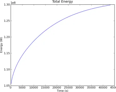
The last statement generates the plot and writes the result into the filetotE.pngwhich can be displayed by (almost) any image viewer. As expected the total energy is constant over time, see Figure (2.4).

Figure 2.4: Example 1b: Total Energy in the Blocks over Time (in seconds)

(27)

2.1.10 Plotting the Temperature Distribution

The scripts referenced in this section are; example01c.py

For plotting the spatial distribution of the temperature we need to modify the strategy we have used for the to-tal energy. Instead of producing a final plot at the end we will generate a picture at each time step which can be browsed as a slide show or composed into a movie. The first problem we encounter is that if we produce an image at each time step we need to make sure that the images previously generated are not overwritten.

To develop an incrementing file name we can use the following convention. It is convenient to put all image files showing the same variable - in our case the temperature distribution - into a separate directory. As part of theosmodule17_python_{provides the}_os.path.join_{command to build file and directory names in a platform} independent way. Assuming that save_path is the name of the directory we want to put the results in the command is;

import os

os.path.join(save_path, "tempT%03d.png"%i )

whereiis the time step counter. There are two arguments to thejoincommand. Thesave_pathvariable is a predefined string pointing to the directory we want to save our data, for example a single sub-folder calleddata would be defined by;

save_path = "data"

while a sub-folder ofdatacalledexample01would be defined by;

save_path = os.path.join("data","example01")

The second argument ofjoin contains a string which is the file name or subdirectory name. We can use the operator%to use the value ofias part of our filename. The sub-string%03dindicates that we want to substitute a value into the name;

• 0means that small numbers should have leading zeroes;

• 3means that numbers should be written using at least 3 digits; and

• dmeans that the value to substitute will be a decimal integer.

To actually substitute the value ofiinto the name write%iafter the string. When done correctly, the output files from this command will be placed in the directory defined bysave_pathas;

17_The_os_{module provides a powerful interface to interact with the operating system, see}_{http://docs.python.org/library/os.}

(28)

blockspyplot001.png blockspyplot002.png blockspyplot003.png ...

and so on.

A sub-folder check/constructor is available inescript. The command;

mkDir(save_path)

will check for the existence ofsave_pathand if missing, create the required directories.

We start by modifying our solution script. Prior to thewhileloop we need to extract our finite solution points to a data object that is compatible withmatplotlib. First we create the node coordinates of the sample points used to represent the temperature as apythonlist of tuples or anumpyarray as requested by the plotting function. We need to convert the arrayxpreviously set asSolution(blocks).getX()into apythonlist and then to a numpyarray. Thex0component is then extracted via an array slice to the variableplx;

import numpy as np # array package. #convert solution points for plotting

plx = x.toListOfTuples()

plx = np.array(plx) # convert to tuple to numpy array

plx = plx[:,0] # extract x locations

(29)

(30)

We use the same techniques provided bymatplotlibas we have used to plot the total energy over time. For each time step we generate a plot of the temperature distribution and save each to a file. The following is appended to the end of thewhileloop and creates one figure of the temperature distribution. We start by converting the solution to a tuple and then plotting this against ourx coordinatesplxwe have generated before. We add a title to the diagram before it is rendered into a file. Finally, the figure is saved to a *.pngfile and cleared for the following iteration. # ... start iteration: while t<tend: i+=1 t+=h mypde.setValue(Y=qH+rhocp/h*T) T=mypde.getSolution() totE=integrate(rhocp*T)

print "time step %s at t=%e days completed. total energy = %e."%(i,t/day,totE)

t_list.append(t) E_list.append(totE)

#establish figure 1 for temperature vs x plots

tempT = T.toListOfTuples() pl.figure(1) #current figure

pl.plot(plx,tempT) #plot solution # add title

pl.axis([0,mx,T1*.9,T2*1.1])

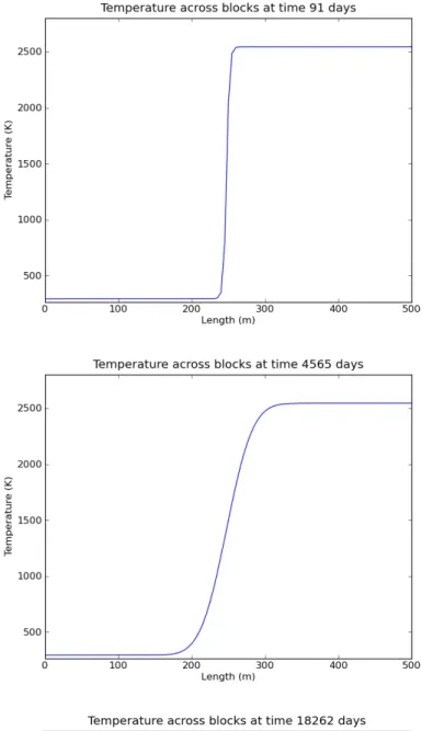
pl.title("Temperature across blocks at time %d days"%(t/day))

#save figure to file

pl.savefig(os.path.join(save_path,"tempT", "blockspyplot%03d.png"%i)) pl.clf() #clear figure

Some results are shown in Figure (2.5).

2.1.11 Making a Video

Our saved plots from the previous section can be cast into a video using the following command appended to the end of the script. Themencodercommand is not available on every platform, so some users need to use an alternative video encoder.

# compile the *.png files to create a *.avi video that shows T change # with time. This operation uses Linux mencoder. For other operating

(31)

# systems it is possible to use your favourite video compiler to

# convert image files to videos.

os.system("mencoder mf://"+save_path+"/tempT"+_{"/*.png -mf type=png:\}

w=800:h=600:fps=25 -ovc lavc -lavcopts vcodec=mpeg4 -oac copy -o \

example01tempT.avi")

2.2 Example 2: One Dimensional Heat Diffusion in an Iron Rod

The scripts referenced in this section are; example02.py

Our second example is of a cold iron bar at a constant temperature ofTref = 20◦C, see Figure (2.6). The

bar is perfectly insulated on all sides with a heating element at one end keeping the temperature at a constant level T0= 100◦C. As heat is applied energy will disperse along the bar via conduction. With time the bar will reach a

constant temperature equivalent to that of the heat source.

Figure 2.6: Example 2: One dimensional model of an Iron bar

This problem is very similar to the example of temperature diffusion in granite blocks presented in the previous Section2.1. Thus, it is possible to modify the script we have already developed for the granite blocks to suit the iron bar problem. The obvious differences between the two problems are the dimensions of the domain and different materials involved. This will change the time scale of the model from years to hours. The new settings are

#Domain related.

mx = 1*m #meters - model length

my = .1*m #meters - model width

ndx = 100 # mesh steps in x direction

ndy = 1 # mesh steps in y direction - one dimension means one element #PDE related

rho = 7874. *kg/m**3 #kg/mˆ{3} density of iron

cp = 449.*J/(kg*K) # J/Kg.K thermal capacity

(32)

kappa = 80.*W/m/K # watts/m.Kthermal conductivity

qH = 0 * J/(sec*m**3) # J/(sec.mˆ{3}) no heat source

Tref = 20 * Celsius # base temperature of the rod

T0 = 100 * Celsius # temperature at heating element

tend= 0.5 * day # - time to end simulation

We also need to alter the initial value for the temperature. Now we need to set the temperature toT0at the left

end of the rod where we havex0 = 0andTref elsewhere. Instead ofwhereNegativefunction we now use

whereZerowhich returns the value one for those sample points where the argument (almost) equals zero and the value zero elsewhere. The initial temperature is set to

# ... set initial temperature ....

T= T0*whereZero(x[0])+Tref*(1-whereZero(x[0]))

2.2.1 Dirichlet Boundary Conditions

In the iron rod model we want to keep the initial temperatureT0on the left side of the domain constant with time.

This implies that when we solve the PDE Equation (2.5), the solution must have the value T0 on the left hand

side of the domain. As mentioned already in Section2.1.3where we discussed boundary conditions, this kind of scenario can be expressed using aDirichlet boundary condition. Some people also use the termconstraintfor the PDE.

To define a Dirichlet boundary condition we need to specify where to apply the condition and determine what value the solution should have at these locations. In escriptwe use q andr to define the Dirichlet boundary conditions for a PDE. The solution uof the PDE is set torfor all sample points whereqhas a positive value. Mathematically this is expressed in the form;

u(x) =r(x)for anyxwithq(x)>0 (2.19)

In the case of the iron rod we can set q=whereZero(x[0])

r=T0

to prescribe the valueT0for the temperature at the left end of the rod wherex0= 0. Here we use thewhereZero

function again which we have already used to set the initial value. Notice thatris set to the constant valueT0for

all sample points. In fact, values ofrare used only whereqis positive. Whereqis non-positive,rmay have any value as these values are not used by the PDE solver.

(33)

To set the Dirichlet boundary conditions for the PDE to be solved in each time step we need to add some statements; mypde=LinearPDE(rod) A=zeros((2,2))) A[0,0]=kappa q=whereZero(x[0]) mypde.setValue(A=A, D=rhocp/h, q=q, r=T0)

It is important to remark here that if a Dirichlet boundary condition is prescribed on the same location as any Neumann boundary condition, the Neumann boundary condition will beoverwritten. This applies to Neumann boundary conditions thatescriptsets by default and those defined by the user.

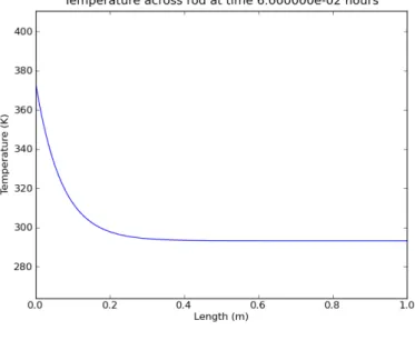
Besides some cosmetic modification this is all we need to change. The total energy over time is shown in Figure (2.7). As heat is transferred into the rod by the heater the total energy is growing over time but reaches a plateau when the temperature is constant in the rod, see Figure (2.8). You will notice that the time scale of this model is several order of magnitudes faster than for the granite rock problem due to the different length scale and material parameters. In practice it can take a few model runs before the right time scale has been chosen18_.

Figure 2.7: Example 2: Total Energy in the Iron Rod over Time (in seconds)

2.3 For the Reader

1. Move the boundary line between the two granite blocks to another part of the domain.

18_{An estimate of the time scale for a diffusion problem is given by the formula} ρcpL20

4κ , seehttp://en.wikipedia.org/wiki/ Fick%27s_laws_of_diffusion

(34)

2. Split the domain into multiple granite blocks with varying temperatures.

3. Vary the mesh step size. Do you see a difference in the answers? What does happen with the compute time? 4. Insert an internal heat source (Hint: The internal heat source is given byqH.)

5. Change the boundary condition for the iron rod example such that the temperature at the right end is kept at a constant levelTref, which corresponds to the installation of a cooling element (Hint: Modifyqandr).

(35)

(36)

(37)

CHAPTER

THREE

Heat Diffusion in Two Dimensions

The scripts referenced in this section are; example03a.py and cblib.py

Building upon our success from the 1D models, it is now prudent to expand our domain by another dimension. For this example we use a very simple magmatic intrusion as the basis for our model. The simulation will be a single event where some molten granite has formed a cylindrical dome at the base of some cold sandstone country rock. Assuming that the cylinder is very long we model a cross-section as shown in Figure (3.1). We will implement the same diffusion model as we have used for the granite blocks in Section2.1but will add the second spatial dimension and show how to define variables depending on the location of the domain. We use onedheatdiff001b.pyas the starting point to develop this model.

3.1 Example 3: Two Dimensional Heat Diffusion for a basic Magmatic

Intrusion

To expand upon our 1D problem, the domain must first be expanded. In fact, we have solved a two dimensional problem already but essentially ignored the second dimension. In our definition phase we create a square domain inxandy1_{that is}₆₀₀_{meters along each side Figure (}_3.1_{). Now we set the number of discrete spatial cells to}₁₅₀ in both directions and the radius of the intrusion to200meters with the centre located at the300meter mark on thex-axis. Thus, the domain variables are;

mx = 600*m #meters - model length

1_In_escript_{the notation}_x

(38)

Figure 3.1: Example 3: 2D model: granitic intrusion of sandstone country rock

my = 600*m #meters - model width

ndx = 150 #mesh steps in x direction

ndy = 150 #mesh steps in y direction

r = 200*m #meters - radius of intrusion

ic = [300*m, 0] #coordinates of the centre of intrusion (meters)

qH=0.*J/(sec*m**3) #our heat source temperature is zero

As before we use

model = Rectangle(l0=mx,l1=my,n0=ndx, n1=ndy)

to generate the domain.

There are two fundamental changes to the PDE that we have discussed in Section2.1. Firstly, because the material coefficients for granite and sandstone are different, we need to deal with PDE coefficients which vary with their location in the domain. Secondly, we need to deal with the second spatial dimension. We can investigate these two modifications at the same time. In fact, the temperature model Equation (2.1) we utilised in Section2.1

applied for the 1D case with a constant material parameter only. For the more general case examined in this chapter, the correct model equation is

ρcp ∂T ∂t − ∂ ∂xκ ∂T ∂x − ∂ ∂yκ ∂T ∂y =qH (3.1)

Notice that for the 1D case we have ∂T_∂y = 0and for the case of constant material parameters _∂x∂ κ=κ∂

∂x thus this

new equation coincides with a simplified model equation for this case. It is more convenient to write this equation 38 3.1. Example 3: Two Dimensional Heat Diffusion for a basic Magmatic Intrusion

(39)

using the∇notation as we have already seen in Equation (2.6);

ρcp

∂T

∂t − ∇ ·κ∇T=qH (3.2)

We can easily apply the backward Euler scheme as before to end up with

ρcp h T (n)_{− ∇ ·}_κ_∇_T(n)₌_q H+ ρcp h T (n−1) (3.3)

which is very similar to Equation (2.9) used to define the temperature update in the simple 1D case. The difference is in the second order derivative term∇ ·κ∇T(n)_{. Under the light of the more general case we need to revisit the}

escriptPDE form as shown in2.16. For the 2D case with variable PDE coefficients the form needs to be read as

− ∂ ∂xA00 ∂u ∂x− ∂ ∂xA01 ∂u ∂y − ∂ ∂yA10 ∂u ∂x− ∂ ∂xA11 ∂u ∂y +Du=f (3.4)

So besides the settingsu=T(n)_,_D₌ ρcp

h andf =qH+ ρcp

h T

(n−1)_{as we have used before (see Equation (}_2.10₎₎

we need to set

A00=A11=κ;A01=A10= 0 (3.5)

The fundamental difference to the 1D case is thatA11is not set to zero butκ, which brings in the second dimension.

It is important to note that the coefficients of the PDE may depend on their location in the domain which does not influence the usage of the PDE form. This is very convenient as we can introduce spatial dependence to the PDE coefficients without modification to the way we call the PDE solver.

A very convenient way to define the matrix Ain Equation (3.5) can be carried out using the Kroneckerδ symbol2_{. The}_escript_function_kronecker_{returns this matrix;}

kronecker(model)=    1 0 0 1    (3.6)

As the argumentmodelrepresents a two dimensional domain the matrix is returned as a2×2matrix (in the case of a three-dimensional domain a3×3matrix is returned). The call

mypde.setValue(A=kappa*kronecker(model),D=rhocp/h)

sets the PDE coefficients according to Equation (3.5).

(40)

We need to check the boundary conditions before we turn to the question: how do we setκ. As pointed out Equation (2.14) makes certain assumptions on the boundary conditions. In our case these assumptions translate to;

−n·κ∇T(n)=−n0·κ

∂T(n)

∂x −n1·κ ∂T(n)

∂y = 0 (3.7)

which sets the normal component of the heat flux−κ·(∂T(n) ∂x ,

∂T(n)

∂y )to zero. This means that the region is

insulated which is what we want. On the left and right face of the domain where we have(n0, n1) = (∓1,0)this

means ∂T_∂x(n) = 0and on the top and bottom on the domain where we have(n0, n1) = (±1,0)this is ∂T

(n)

∂y = 0.

3.2 Setting variable PDE Coefficients

Now we need to look into the problem of how we define the material coefficientsκandρcp depending on their

location in the domain. We can make use of the technique used in the granite block example in Section2.1to set up the initial temperature. However, the situation is more complicated here as we have to deal with a curved interface between the two sub-domains.

Prior to setting up the PDE, the interface between the two materials must be established. The distances≥0

between two points[x, y]and[x0, y0]in Cartesian coordinates is defined as:

(x−x0)2+ (y−y0)2=s2 (3.8)

If we define the point[x0, y0]asicwhich denotes the centre of the semi-circle of our intrusion, then for all the

points[x, y]in our model we can calculate a distance toic. All the points that fall within the given radiusrof our intrusion will have a corresponding values < rand all those belonging to the country rock will have a value s > r. By subtractingrfrom both of these conditions we finds−r <0for all intrusion points ands−r >0for all country rock points. Defining these conditions within the script is quite simple and is done using the following command:

bound = length(x-ic)-r #where the boundary will be located

This definition of the boundary can now be used with thewhereNegativecommand again to help define the material constants and temperatures in our domain. Ifkappaiandkappacare the thermal conductivities for the intrusion material granite and for the surrounding sandstone, then we set;

x=Function(model).getX() bound = length(x-ic)-r

kappa = kappai * whereNegative(bound) + kappac * (1-whereNegative(bound)) mypde.setValue(A=kappa*kronecker(model))

(41)

Notice that we are using the sample points of theFunctionfunction space as expected for the PDE coefficient A3. The corresponding statements are used to setρcp.

Our PDE has now been properly established. The initial conditions for temperature are set out in a similar manner:

#defining the initial temperatures.

x=Solution(model).getX() bound = length(x-ic)-r

T= Ti*whereNegative(bound)+Tc*(1-whereNegative(bound))

whereTiandTcare the initial temperature in the regions of the granite and surrounding sandstone, respectively. It is important to notice that we resetxandboundto refer to the appropriate sample points of a PDE solution4_.

3.3 Contouring

escript

Data using

matplotlib

.

To complete our transition from a 1D to a 2D model we also need to modify the plotting procedure. As before we usematplotlibto do the plotting in this case a contour plot. For 2D contour plotsmatplotlibexpects that the data are regularly gridded. We have no control over the location and ordering of the sample points used to represent the solution. Therefore it is necessary to interpolate our solution onto a regular grid.

In Section2.1.10we have already learned how to extract thexcoordinates of sample points asnumpyarray to hand the values tomatplotlib. This can easily be extended to extract both thexand theycoordinates;

import numpy as np

def toXYTuple(coords):

coords = np.array(coords.toListOfTuples()) #convert to Tuple

coordX = coords[:,0] #X components.

coordY = coords[:,1] #Y components. return coordX,coordY

For convenience we have put this function intoclib.pyso we can use this function in other scripts more easily. We now generate a regular100×100grid over the domain (mxandmy are the dimensions in thexandy directions) which is done using thenumpyfunctionlinspace.

from clib import toXYTuple

# get sample points for temperature as for contouring

coordX, coordY = toXYTuple(T.getFunctionSpace().getX())

# create regular grid

xi = np.linspace(0.0,mx,75)

3_{For the experienced user: use}_{x=mypde.getFunctionSpace("A").getX()}_. 4_{For the experienced user: use}_{x=mypde.getFunctionSpace("r").getX()}_.

(42)

yi = np.linspace(0.0,my,75)

The values[xi[k], yi[l]]are the grid points.

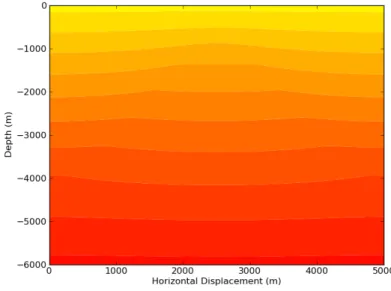
The remainder of our contouring commands resides within awhileloop so that a new contour is generated for each time step. For each time step the solution must be re-gridded formatplotlibusing thegriddata function. This function interprets irregularly located valuestempTat locations defined bycoordXandcoordY as values at the new coordinates of a rectangular grid defined byxiandyi. The output iszi. It is now possible to use the contourffunction which generates colour filled contours. The colour gradient of our plots is set via the commandpl.matplotlib.pyplot.autumn(), other colours are listed on thematplotlibweb page5_{. Our results are then contoured, visually adjusted using the}_matplotlib_{functions and then saved to a file.} pl.clf()clears the figure in readiness for the next time iteration.

#grid the data.

zi = pl.matplotlib.mlab.griddata(coordX,coordY,tempT,xi,yi)

# contour the gridded data, plotting dots at the randomly spaced data points.

pl.matplotlib.pyplot.autumn() pl.contourf(xi,yi,zi,10)

CS = pl.contour(xi,yi,zi,5,linewidths=0.5,colors=’k’) pl.clabel(CS, inline=1, fontsize=8)

pl.axis([0,600,0,600])

pl.title("Heat diffusion from an intrusion.") pl.xlabel("Horizontal Displacement (m)") pl.ylabel("Depth (m)")

pl.savefig(os.path.join(save_path,"Tcontour%03d.png") %i) pl.clf()

The functionpl.contouris used to add labelled contour lines to the plot. The results for selected time steps are shown in Figure (3.2).

3.4 Advanced Visualisation using VTK

The scripts referenced in this section are; example03b.py

An alternative approach tomatplotlibfor visualisation is the usage of a package which is based on the Vi-sualization Toolkit (VTK) library6. There is a variety of packages available. Here we use the packageMayavi27as an example.

5_see_{http://matplotlib.sourceforge.net/api/} 6_see_{http://www.vtk.org/}

7_see_{http://code.enthought.com/projects/mayavi/}

(43)

Mayavi2is an interactive, GUI driven tool which is really designed to visualise large three dimensional data sets wherematplotlibis not suitable. But it is also very useful when it comes to two dimensional problems. The decision of which tool is the best can be subjective and users should determine which package they require and are most comfortable with. The main difference between using Mayavi2 (or other VTK based tools) and matplotlibis that the actual visualisation is detached from the calculation by writing the results to external files and importing them intoMayavi2. In 3D the best camera position for rendering a scene is not obvious before the results are available. Therefore the user may need to try different settings before the best is found. Moreover, in many cases a 3D interactive visualisation is the only way to really understand the results (e.g. using stereographic projection).

To write the temperatures at each time step to data files in the VTK file format one needs to importsaveVTK from theesys.weipamodule and call it:

from esys.weipa import saveVTK

while t<=tend: i+=1 #counter t+=h #current time mypde.setValue(Y=qH+T*rhocp/h) T=mypde.getSolution() saveVTK(os.path.join(save_path,"data.%03d.vtu"%i, T=T)

The data files, e.g. data.001.vtu, contain all necessary information to visualise the temperature and can be directly processed byMayavi2. Note that there is no re-gridding required. The file extension.vtuis automatically added if not supplied tosaveVTK.

After you run the script you will find the result filesdata.*.vtuin the result directorydata/example03. Run the command

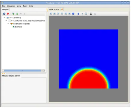
>> mayavi2 -d data.001.vtu -m Surface &

from the result directory. Mayavi2will start up a window similar to Figure (3.3). The right hand side shows the temperature at the first time step. To show the results at other time steps you can click at the item VTK XML file (data.001.vtu) (timeseries)at the top left hand side. This will bring up a new window similar to the window shown in Figure (3.4). By clicking at the arrows in the top right corner you can move forwards and backwards in time. You will also notice the textTnext to the itemPoint scalars name. The nameT

corresponds to the keyword argument nameTwe have used in thesaveVTKcall. In this menu item you can select other results you may have written to the output file for visualisation.

For the advanced user: Using thematplotlibto visualise spatially distributed data is not MPI compatible. However, thesaveVTKfunction can be used with MPI. In fact, the function collects the values of the sample

(44)

points spread across processor ranks into a single file. For more details on writing scripts for parallel computing please consult theuser’s guide.

(45)

Figure 3.2: Example 3a: 2D model: Total temperature distribution (T) at time step1,20and200. Contour lines show temperature.

(46)

Figure 3.3: Example 3b:Mayavi2start up window

Figure 3.4: Example 3b:Mayavi2data control window

(47)

CHAPTER

FOUR

Complex Geometries

4.1 Steady-state Heat Refraction

In this chapter we demonstrate how to handle more complex geometries.

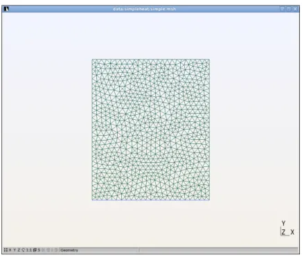
Steady-state heat refraction will give us an opportunity to investigate some of the richer features that theescript package has to offer. One of these isesys.pycad. The advantage of usingesys.pycadis that it offers an easy method for developing and manipulating complex domains. In conjunction withesys.pycad.gmshwe can generate finite element meshes that conform to our domain’s shape providing accurate modelling of interfaces and boundaries. Another useful function ofesys.pycadis that we can tag specific areas of our domain with labels as we construct them. These labels can then be used inescriptto define properties like material constants and source locations.

We proceed in this chapter by first looking at a very simple geometry. Whilst a simple rectangular domain is not very interesting the example is elaborated upon later by introducing an internal curved interface.

4.2 Example 4: Creating the Domain with

esys.pycad

The scripts referenced in this section are; example04a.py

We modify the example in Chapter3in two ways: we look at the steady state case with slightly modified boundary conditions and use a more flexible tool to generate the geometry. Let us look at the geometry first.

We want to define a rectangular domain of width5kmand depth6km below the surface of the Earth. The domain is subject to a few conditions. The temperature is known at the surface and the basement has a known heat

(48)

flux. Each side of the domain is insulated and the aim is to calculate the final temperature distribution.

Inesys.pycadthere are a few primary constructors that build upon each other to define domains and bound-aries. The ones we use are:

from esys.pycad import *

Point() #Create a point in space.

Line() #Creates a line from a number of points.

CurveLoop() #Creates a closed loop from a number of lines.

PlaneSurface() #Creates a surface based on a CurveLoop

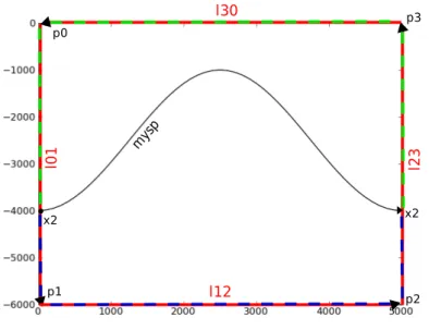
So to construct our domain as shown in Figure (4.1), we first need to create the corner points. From the corner points we build the four edges of the rectangle. The four edges then form a closed loop which defines our domain as a surface. We start by inputting the variables we need to construct the model.

width=5000.0*m #width of model

depth=-6000.0*m #depth of model

p1 p4 p3 p2 l 0 1 l 2 3 l30 l12

Figure 4.1: Example 4: Rectangular Domain foresys.pycad

The variables are then used to construct the four corners of our domain, which from the origin has the dimen-sions of5000meters width and−6000meters depth. This is done with thePoint()function which accepts x, y and z coordinates. Our domain is in two dimensions so z should always be zero.

# Overall Domain

p0=Point(0.0, 0.0, 0.0) p1=Point(0.0, depth, 0.0) p2=Point(width, depth, 0.0) p3=Point(width, 0.0, 0.0)

The escript cookbook: Release - 3.2.1 (r3613)

The

escript

COOKBOOK

Release - 3.2.1

(r3613)

Antony Hallam, Lutz Gross, et al.

September 28, 2011

Earth Systems Science Computational Centre (ESSCC)

School of Earth Sciences

The University of Queensland

Brisbane, Australia

Researchers and Developers

Contents

CHAPTER

ONE

Introduction

1.1

Why

escript

?

1.2

How to use this Cookbook

1.3

Quickstart

1.4

Escript and Python Basics

1.4.1

The

esys

Modules

CHAPTER

TWO

Getting Started with Heat Diffusion

2.1

Example 1: One Dimensional Heat Diffusion in Granite

2.1.1

1D Heat Diffusion Equation

2.1.2

PDEs and the General Form

2.1.3

Boundary Conditions

2.1.4

Outline of the Implementation

2.1.5

The Domain Constructor in

escript

Input Parameters

Domain

Boundary Values

Nodes

Coefficients

2.1.6

A Clarification for the 1D Case

2.1.7

Developing a PDE Solution Script

2.1.8

Running the Script

2.1.9

Plotting the Total Energy

2.1.10

Plotting the Temperature Distribution

2.1.11

Making a Video

2.2

Example 2: One Dimensional Heat Diffusion in an Iron Rod

2.2.1

Dirichlet Boundary Conditions

2.3

For the Reader

CHAPTER

THREE

Heat Diffusion in Two Dimensions

3.1

Example 3: Two Dimensional Heat Diffusion for a basic Magmatic

Intrusion

3.2

Setting variable PDE Coefficients

3.3

Contouring