On the Approximability of Adjustable Robust Convex
Optimization under Uncertainty
Dimitris Bertsimas · Vineet Goyal
May 12, 2012
Abstract In this paper, we consider adjustable robust versions of convex optimiza-tion problems with uncertain constraints and objectives and show that under fairly general assumptions, a static robust solution provides a good approximation for these adjustable robust problems. An adjustable robust optimization problem is usually in-tractable since it requires to compute a solution for all possible realizations of uncertain parameters, while an optimal static solution can be computed efficiently in most cases if the corresponding deterministic problem is tractable. The performance of the optimal static robust solution is related to a fundamental geometric property, namely, the sym-metryof the uncertainty set. Our work allows for the constraint and objective function coefficients to be uncertain and for the constraints and objective functions to be convex, thereby providing significant extensions of the results in [8] and [9] where only linear objective and linear constraints were considered. The models in this paper encompass a wide variety of problems in revenue management, resource allocation under uncer-tainty, scheduling problems with uncertain processing times, semidefinite optimization among many others. To the best of our knowledge, these are the first approximation bounds for adjustable robust convex optimization problems in such generality.
Keywords Robust Optimization·Static Policies·Adjustable Robust Policies
V. Goyal is supported by NSF Grant CMMI-1201116. D. Bertsimas
Sloan School of Management and Operations Research Center
Massachusetts Institute of Technology Cambridge, MA 02139
E-mail: [email protected] V. Goyal
Dept of Industrial Engineering and Operations Research Columbia University
New York, NY 10027
1 Introduction
In most real world problems, problem parameters are uncertain at the optimization or decision-making phase. Solutions obtained via deterministic optimization might be sensitive to even small perturbations in the problem parameters that might render them highly infeasible or suboptimal. Stochastic optimization was introduced by Dantzig [12] and Beale [1], and since then has been extensively studied in the literature to address the uncertainty in problem parameters. A stochastic optimization approach assumes a probability distribution over the uncertain parameters and seeks to optimize the expected value of the objective function. We refer the reader to several textbooks including Infanger [18], Kall and Wallace [19], Prekopa [21], Shapiro [22], Shapiro et al. [23] and the references therein for a comprehensive review of stochastic optimization. While the stochastic optimization approach has its merits, it is by and large com-putationally intractable even when the constraint and objective functions are linear. Shapiro and Nemirovski [24] give hardness results for two-stage and multi-stage stochas-tic optimization problems where they show that the multi-stage stochasstochas-tic optimization problem is computationally intractable even if approximate solutions are desired. Dyer and Stougie [13] show that a multi-stage stochastic optimization problem where the distribution of uncertain parameters in any stage also depends on the decisions in past stages is PSPACE-hard. Even for the stochastic problems that can be solved efficiently, it is difficult to estimate the probability distributions of the uncertain parameters from historical data to formulate the problem.
More recently, the robust optimization approach has been considered to address optimization under uncertainty and has been studied extensively (see Ben-Tal and Nemirovski [4], [5] and [6], El Ghaoui and Lebret [14], Bertsimas and Sim [10, 11], Goldfarb and Iyengar [16]). In a robust optimization approach, the uncertain parame-ters are assumed to belong to some uncertainty set and the goal is to construct a single (static) solution that is feasible for all possible realizations of the uncertain parame-ters from the set and optimizes the worst-case objective. We point the reader to the survey by Bertsimas et al. [7] and the book by Ben-Tal et al. [2] and the references therein for an extensive review of the literature in robust optimization. This approach is significantly more tractable as compared to a stochastic optimization approach and the robust problem is equivalent to the corresponding deterministic problem in com-putational complexity for a large class of problems and uncertainty sets (Bertsimas et al. [7]). However, the robust optimization approach may have the following drawbacks. Since it optimizes over the worst-case realization of the uncertain parameters, it may produce conservative solutions that may not perform well in the expected value sense. Moreover, the robust approach computes a single (static) solution even for a multi-stage problem with several stages of decision-making as opposed a fully-adjustable solution where decisions in each stage depend on the actual realizations of the parameters in past stages. This may further add to the conservativeness.
Another approach is to consider solutions that are fully-adjustable in each stage and depend on the realizations of the parameters in past stages and optimize over the worst case. Such solution approaches have been considered in the literature and referred to as adjustable robust policies (see Ben-Tal et al. [3] and the book by Ben-Tal et al. [2] for a detailed discussion of these policies). Unfortunately, the adjustable robust problem is computationally intractable in general. Feige et al. [15] show that it is hard to approximate even a two-stage set covering linear program within a factor ofΩ(logn) for a general uncertainty set. Bertsimas and Goyal [8] show that astatic solution (a
single solution that is feasible for all possible realizations of the uncertain parameters) is a 2-approximation for the adjustable robust as well as a stochastic optimization problem with linear constraints and objective with right hand side uncertainty if the uncertainty set belongs to the non-negative orthant and is perfectlysymmetricsuch as a hypercube or an ellipsoid. Bertsimas et al. [9] give two significant generalizations of the result in [8] where they show that the performance of the static solution for the adjustable robust and the stochastic problem depends on a fundamental geometric property of the uncertainty namely symmetry. The authors consider a generalized notion of symmetry introduced in Minkowski [20], where the symmetry of a convex set is a number between 0 and 1. The symmetry of a set being equal to one implies that it is perfectly symmetric (such as an ellipsoid). Furthermore, they also generalize the static robust solution policy to a finitely adjustable solution policy for the multi-stage stochastic and adjustable robust optimization problems and give a similar bound on its performance that is related to the symmetry of the uncertainty sets.
The models in [8] and [9] consider only covering constraints of the form aTx ≥ b, a ∈ Rn and b ≥ 0 and the uncertainty appears only in the right hand side of the constraints. While these are fairly general models, they do not handle packing constraints and uncertainty in constraint coefficients. They do not capture several im-portant applications such as revenue management and resource allocation problems under uncertain resource requirements, where we have packing constraints and uncer-tainty in constraint coefficients. In a typical revenue management problem, we need to allocate of scarce resources to a demand with uncertain resource requirements such that the total revenue is maximized. As an example, consider a multi-period problem where there is a single resource with capacityh∈R+, and in each periodk= 1, . . . , T,
a demand arrives and requires an uncertain amount,bk of that resource and we obtain
revenuedk per unit of demand satisfied. The goal in each period is to decide on the
fraction of demand that should be satisfied such that the worst case revenue over all future resource requirements is maximized.
Let xk be the fraction of demand in period k that is satisfied for k = 1, . . . , K.
Note that in periodk, we observe the resource requirements for demands in all periods up to period k but do not know the resource requirements for future demands. The multi-period adjustable robust revenue maximization problem can now be formulated as follows. maxd1x1(b1) + min b2∈U2 max x2(b1,b2) d2·x2(b1, b2) +. . . + min bK∈UK max xK(b1,...,bK) dK·xK(b1, . . . , bK)). . . K X k=1 bk·xk(b1, . . . , bk)≤h, ∀bk∈ Uk, k= 2, . . . , K 0≤xk(b1, . . . , bk)≤1, ∀k= 1, . . . , K. (1.1)
In order to address such problems, we need to consider linear optimization problems under constraint and objective coefficient uncertainty. Moreover, the framework in [8] and [9] covers linear optimization problems, but not general convex optimization problems. In this paper, we study adjustable robust versions of fairly general convex optimization problems under uncertain convex constraints and objective. In particu-lar, these include linear packing problems under constraint and objective uncertainty. While computing an optimal adjustable robust solution is intractable, we show that an
optimal static robust solution provides a good approximation for the adjustable robust problem.
1.1 Models and Notation
We study the following adjustable robust version of a two-stage convex optimization problemΠARcons(U) under uncertain constraints.
zARcons(U) = max
x∈Xf1(x) + minu∈U y(maxu)∈Y f2 y(u)
gi(x,y(u),u)≤ci, ∀u∈ U, ∀i∈I,
(1.2)
where U ⊂ Rp+ is a compact convex set, I is the set of indices for the constraints,
ci ∈ R+ for all i ∈ I and functions f1 : Rn+1 → R+, f2 : R+n2 → R+ and gi : Rn+1+n2+p→R+, i∈I satisfy the following conditions:
(A1) The functionf1is concave and satisfiesf1(0) = 0.
(A2) f2is concave and satisfiesf2(0) = 0.
(A3) For alli∈I,gi is convex inxandy, concave and increasing inuand satisfies,
g(0,0,u) = 0, ∀u∈ U ∂gi
∂uj
≥0, ∀j= 1, . . . , p, ∀x∈X,y∈Y
Moreover, given ˆx∈X and ˆy∈Y, the problem maxu∈Ugi(ˆx,yˆ,u) is solvable in
polynomial time.
(A4) SetsX andY are convex and0∈X,0∈Y.
Assumptions(A1)-(A4)are fairly general and model two-stage adjustable robust versions of a large class of deterministic convex optimization problems. In Section 1.2 we illustrate that they hold for several important application areas. The assumption that the objective functionsf1 andf2are concave and the constraint functionsgi(·), i∈I
are convex are necessary for the above problem to be a convex optimization problem. The assumption thatf1(0) =f2(0) = 0 is without loss of generality as we can always
translatef1 andf2 to satisfy this condition. In addition, we assume that for alli∈I,
giis an increasing concave function ofuand g(0,0,u) = 0 for allu∈ U. We require
the concavity assumption for the tractability of the static-robust problem.
Note thatΠARcons(U) is a two-stage problem wherexdenotes the first-stage decision. The uncertain parametersu∈ U materialize after the first-stage decisions have been made and we can then select the second-stage or recourse decisiony(u) that depends onu. The goal is to findx ∈X such that for allu ∈ U there is a feasible recourse decisiony(u) and the total objective:f1(x) +f2(y(u)) is maximized over the
worst-case choice of u ∈ U. We note that in ΠARcons(U), we only model uncertainty in the constraints (for alli∈ I, the constraint functiongi is a function ofu in addition to
the decision variablesx,y(u)). There is no uncertainty in the objective function. We also consider the problem where uncertainty appears in both constraints as well as objective functions. This model is described in (4.1).
Since computing an optimal fully-adjustable solution for (1.2) is intractable in general even whenf1, f2andgi, i∈Iare linear (see Dyer and Stougie [13]), we consider
the corresponding static-robust problemΠRob(U):
zRobcons(U) = max
x∈X,y∈Y f1(x) +f2(y)
gi(x,y,u)≤ci, ∀u∈ U, ∀i∈I,
(1.3)
We show that it is tractable to compute an optimal static robust solution to (1.3) and we compare the performance of an optimal static robust solution for the adjustable robust problem (1.2). Note that under assumptions (A1)−(A4), both (1.2) and (1.3) are feasible as x = 0,y(u) = 0 for all u ∈ U is a feasible solution for (1.2) and
x=0,y=0is a feasible solution for (1.3). Therefore, zconsAR(U)≥z
cons
Rob(U)≥0.
1.2 Applications
In this section, we illustrate the wide modeling flexibility of (4.1) by placing a variety of problem domains in this framework.
1.2.1 Two-Stage Linear Optimization under Constraint Uncertainty
We first consider the classical two-stage adjustable robust linear maximization problem with uncertainty in the constraint coefficients.
zARLin(U) = maxcTx+ min
B∈U y(maxB)∈Y d T y(B) Ax+By(B)≤h ∀B∈ U x≥0 y(B)≥0, (1.4) where A ∈ Rm×n1
+ is the first-stage constraint matrix, B is the uncertain
second-stage constraint matrix, c ∈ Rn1
+, d ∈ R n2
+ and h ∈ R m
+. In the framework (1.2),
f1(x) =cTxthat satisfies(A1),f2(y(B)) =dTythat satisfies(A2), and
gi(x,y,B) = n1 X j=1 Aijxj+ n2 X j=1 Bijyj, i= 1, . . . , m,
that satisfies(A3)as it is convex (linear) inxandyand concave (linear) and increasing inB sincex≥0,y≥0 andB∈Rm+×n2. Before discussing next several applications
of the framework of (1.4) we note that we can not model a linear covering constraint in the framework (1.2), i.e., a constraint of the formaTx+uTy≥1. To model this constraint in (1.2), we require
g(x,y,u) = 1−aTx−uTy,
and the constraint can be formulated asg(x,y,u) ≤0. However, in this case gdoes not satisfy (A3) as g(0,0,u) 6= 0. Even with this limitation, we are able to model
many interesting and important applications that can not be formulated using models in [8] and [9].
Revenue Management.We can model many revenue management problems in the framework (1.4) as discussed briefly earlier. Here, we formulate a two-stage version of the revenue management problem discussed in (1.1) in the framework (1.4) and we consider the case where each demand possibly requires multiple resources in uncertain amounts instead of a single resource. Suppose there aremresources with finite capacity
h∈ Rm+ and two demand types: D1 (|D1|=n1) and D2 (|D2|=n2). DemandsD1
have a known resource requirement given by a matrixA∈ Rm×n1 (A
ij denotes the
amount of resourceirequired per unit of demandj) andcj∈R+is the revenue per unit
of satisfied demandj ∈ D1. The demands D2 have uncertain resource requirements
given by a matrixB∈ U anddj is the revenue per unit of satisfied demandj∈D2.
The goal is to decide the optimal fraction of demandsD1 that must be satisfied such
that the total worst case revenue is maximized.
To formulate this revenue management problem in the two-stage framework of (1.4), let xj,j= 1, . . . , n1 denote the fraction of demandj ∈D1 satisfied and the
second-stage variablesyj(B), j= 1, . . . , n2 denote the fraction of demandj ∈D2 satisfied.
The right-hand side of the constraints, h ∈ Rm+, is the capacity vector of different
resources. Also,
X = [0,1]n, Y = [0,1]n.
With these parameters, the problem (1.4) formulates the above two-stage revenue man-agement problem. This formulation can be extended to a multi-stage problem and therefore, we can model a multi-stage resource allocation problem where there are multiple demand types and all demands of typej arrive in stage j after irrevocable allocation decisions have been made for demand types 1, . . . , j−1.
Production Planning. We can formulate production planning problems under un-certain production requirements as a special case of (1.4). In a production planning problem, we need to producen different products from m raw materials. Productj generates a revenue ofdjper unit for allj= 1, . . . , nandhidenotes the amount of raw
materiali available for alli= 1, . . . , m. If matrixB ∈ Rm×n denotes the uncertain raw material requirements for all products, the robust production planning problem can be formulated in the framework (1.4) withA= 0.
Network Design. We can also model a network design problem in the framework (1.4) where the goal is to decide on edge capacities for satisfying an uncertain demand in the framework of (1.4). In particular, consider the following problem: given an undirected graphG= (V, E), letce be the cost of one unit of capacity anduebe the maximum
possible capacity of edgee∈E. For anyi, j∈V,rij is the uncertain demand fromito
jthat realizes in the second-stage and let dij be the profit obtained from one unit of
flow fromitoj. The goal is to decide on the capacity of the edges in the first stage and the flow in the second-stage so that the total profit is maximized. This network design problem arises in many important applications including capacity planning problems under uncertain demand.
Let xe denote the fraction of total edge capacityuethat is not bought (recall we
are modeling in a maximization framework). Therefore, for all edges e∈E, (1−xe)
is the fraction of edge capacity bought. LetPij denote the set of paths fromitojfor
demand vector isr. We can formulate the network design problem as follows. maxcTx+ min r∈U X i,j∈V dij X P∈Pij fP(r) uexe+ X i,j∈V X P∈Pij:e∈P rijfP(r)≤ue, ∀e∈E 0≤fP≤1, ∀P∈ Pij,∀i, j∈V,
which falls within the framework (1.4).
1.2.2 Quadratically Constrained Problems
In this section, we formulate quadratically constrained problems under uncertainty in the constraints in the framework of (1.2). Consider the following two-stage maximiza-tion problem,ΠARQuad,
zARQuad= max x c T x+ min Q∈U ymax(Q) d T y(Q) xTP x+y(Q)TQy(Q)≤t, ∀Q∈ U x∈Rn+1 y(Q)∈Rn2 +, (1.5) whereU ⊂Sn2 + ∩R n2×n2
+ is the set of uncertain valuesQ∈S n2 + ∩R n2×n2 + andP ∈S n1 +
(S+n denotes the set of symmetric positive semidefinite matrices in dimensionn×n). In the framework of (1.2),u=Qand we have the following functions:
f1(x) =cTx,
f2(y) =dTy,
g(x,y,Q) =xTP x+yTQy.
The objective functions f1, f2 are concave (linear) and satisfy (A1) and (A2). The
constraint function,g is convex inx andy since P andQ are positive semidefinite, and concave (linear) inQ. Also,g(0,0,Q) = 0 for allQ∈ U and it is increasing inQ
as
∂g(x,y,Q) ∂Qij
=yiyj≥0, ∀i, j= 1, . . . , n2,∀x,y≥0.
Therefore,gsatisfies Assumption(A3)and problem (1.5) can be modeled in the frame-work of (1.2). An example of (1.5) includes a portfolio optimization problem where the covariance matrix is uncertain and the goal is to find a portfolio such that the return is maximized and the worst-case variance is at most a given thresholdt. Since this is a one-period problem and there is no recourse decision unlike (1.5), we can formulate it as a static-robust problem in the framework of (1.3) where x= 0,y denotes the portfolio vector, andu=QwhereQis the uncertain covariance matrix. As above, the functionsf2 andgare defined as
1.2.3 Semidefinite Programming
In this section, we formulate semidefinite optimization problems under uncertain con-straints in the framework of (1.2). Consider the following two-stage maximization prob-lem,ΠARSDP:
zARSDP= max
X C·X+ minQ∈U Ymax(Q) D·Y(Q) P·X+Q·Y(Q)≤t, ∀Q∈ U X∈Sn1 + ∩R n1×n1 + Y(Q)∈Sn2 + ∩R n2×n2 + , ∀Q∈ U, (1.6) whereU ⊂Rn2×n2 + andP ∈R n1×n1
+ . Note thatC·X denotes the trace of matrices C andX. In the general framework of (1.2), we have the following functions:
f1(X) =C·X,
f2(Y) =D·Y,
g(X,Y,Q) =P·X+Q·Y.
The functionsf1, f2 are linear functions and satisfy(A1) and (A2). The constraint
functiongis linear inX,Y and also inu=Q. Also,g(0,0,Q) = 0 for allQ∈ Uand gis increasing inu=Qas ∂g ∂Qij =Yij≥0, ∀i, j= 1, . . . , n2,∀Y ∈Sn+2∩R n2×n2 + .
Therefore,gsatisfies Assumption(A3).
2 Contributions
In this paper, we show that the two-stage adjustable robust convex optimization prob-lem under uncertainty as defined in (1.2) can be well approximated by an optimal solution to the corresponding robust version defined in (1.3) under Assumptions (A1)-(A4). Furthermore, we show that an optimal static-robust solution can be computed in polynomial time. We relate the performance of the static robust solution for the adjustable robust problems to fundamental geometric properties of the uncertainty set, namely, symmetry and the translation factor. Let us introduce these geometric properties in order to discuss the results further.
Symmetry of a convex set.Given a nonempty compact convex setU ⊂Rmand a
pointu∈ U, we define the symmetry ofuwith respect toU as follows:
sym(u,U) := max{α≥0 :u+α(u−u0)∈ U, ∀u0∈ U }. (2.1) Then, the symmetry ofU is defined as follows.
sym(U) = max
u∈U sym(u,U), (2.2)
and the maximizer of the above quantity is referred to as thepoint of symmetryofU. This notion of symmetry was introduced in [20]. In general, 1/m≤sym(U)≤1 and if the setU is absolutely symmetricsym(U) = 1.
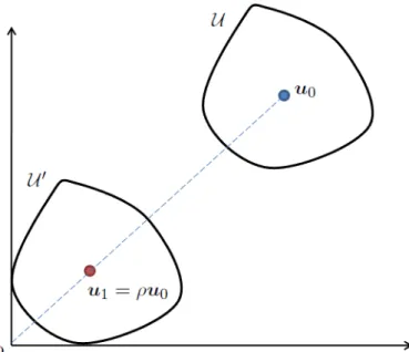
The translation factorρ(u,U).For a convex compact setU ⊂Rm+, following [9], we
define atranslation factor ρ(u,U), the translation factorof u∈ U with respect toU, as follows.
ρ(u,U) = min{α∈R+| U −(1−α)·u⊂Rm+}.
In other words,U0 :=U −(1−ρ)u is the maximum possible translation ofU in the direction −u such thatU0 ⊂Rm+. Figure 1 gives a geometric picture. Note that for
α= 1,U −(1−α)·u=U ⊂Rm+. Therefore, 0< ρ≤1. Andρapproaches 0, when the
setUmoves away from the origin. If there existsu∈ Usuch thatuis at the boundary ofRm+, thenρ= 1. We denote
ρ(U) :=ρ(u0,U), whereu0 is the symmetry point of the setU.
Fig. 1 Geometry of the translation factor.
For the two-stage adjustable robust convex optimization problem,ΠARcons(U) as de-fined in (1.2) where the constraints are uncertain, we show that
zRobcons(U)≤z
cons AR(U)≤ 1 +ρ s
·zRobcons(U),
where zconsRob(U) is the objective value of an optimal static robust solution of (1.3) and s = sym(U) and ρ = ρ(U) are the symmetry and the translation factors of the uncertainty set U. In particular, if the uncertainty setU is symmetric (such as a hypercube, ellipsoid, or a norm-ball), the bound is 2, i.e., the objective value of the optimal adjustable robust solution is at most twice the objective value of an optimal static-robust solution.
We note that most commonly used uncertainty sets are absolutely symmetric. For instance, a parameter uncertainty is very commonly modeled as an interval leading to a hypercube uncertainty set. If we want to avoid possibly conservative corner points in the uncertainty sets, we consider uncertainty sets like ellipsoids and other norm-balls which are also absolutely symmetric. Therefore, an optimal static robust solution that can be computed efficiently provides a good approximation for the adjustable robust problem. This bounds are similar to the bounds presented in [8] and [9] for the performance of a static robust solution for adjustable robust linear minimization problems where the uncertainty appears in the right hand side of the constraints. However, the models studied in this paper are very general and address uncertain convex constraints and objectives as opposed to just linear problems. To the best of our knowledge, these are the first approximation bounds for adjustable robust convex optimization problems in such generality.
The rest of the paper is structured as follows. In Section 3, we show that for two-stage adjustable robust convex optimization problems under constraint uncertainty only, we show that the static solution provides a good approximation under fairly gen-eral assumptions. We further show in Section 3.1 that an optimal static solution can be arbitrarily worse than an optimal fully-adjustable solution for stochastic optimization problems under constraint uncertainty even for a linear model. In Section 4, we extend the results to incorporate uncertainty both in constraints and the objective. In Section 5, we extend further the results to multi-stage problems.
3 Two-stage Adjustable Robust Convex Optimization
In this section, we prove the following bound on the performance of static robust solutions with respect to an optimal fully-adjustable solution.
Theorem 1 Consider the problem defined in (1.2)and the corresponding robust prob-lem defined in (1.3). Lets=sym(U)andρ=ρ(U). Then, under Assumptions (A1)-(A4)
zRobcons(U)≤z
cons AR(U)≤ 1 +ρ s
·zRobcons(U).
In preparation of the proof of Theorem 1 we present several lemmas.
Lemma 1 (Bertsimas et al. [9]) Let U ⊂Rp+ be a compact convex set and letu0 be the point of symmetry ofU. Then,
u≤ 1 + ρ(U) sym(U) u0, ∀u∈ U. (3.1)
Lemma 2 For any0≤α≤1,x∈X,y∈Y, u∈ U, (a) Under Assumption (A1),f1(αx)≥αf1(x).
(b) Under Assumption (A2),f2(αy)≥αf2(y).
(c) Under Assumption (A3), for alli∈I,gi(αx, αy,u)≤αgi(x,y,u).
Proof (a) Recall that f1 is concave and f1(0) = 0 from(A1). Therefore, for any
0≤α≤1,
f1(αx) =f1((1−α)0+αx)
≥(1−α)f1(0) +αf1(x)
where the second last inequality follows from concavity of f1 and the last equation
follows asf1(0) = 0. A similar argument also proves part(b), i.e.,
f2(αy)≥αf2(y).
(c) For any i ∈ I, under Assumption (A3) gi is jointly convex in x and y and
gi(0,0,u) = 0 for allu∈ U. Therefore, for any 0≤α≤1,
gi(αx, αy,u) =gi (1−α)(0,0,u) +α(x,y,u)
≤(1−α)gi(0,0,u) +αgi(x,y,u)
=αgi(x,y,u).
Lemma 3 For anyβ≥1,x∈X,y∈Y,u∈ U and under Assumption(A3) gi(x,y, βu)≤βgi(x,y,u).
Proof Sincegi is concave and increasing inu, we have
gi(x,y,u) =gi 1− 1 β x,y,0+1 β x,y, βu ≥ 1−1 β gi(x,y,0) + 1 βgi(x,y, βu) ≥ 1 βgi(x,y, βu),
where the second last inequality follows as gi is concave inu and the last inequality
follows asgi(x,y,0)≥0 for allx∈X,y∈Y.
Proof of Theorem 1 Letu0be the point of symmetry ofU (that is the maximizer
in (2.2)) ands = sym(u0,U). Suppose x∗,y∗(u) for allu ∈ U be an optimal fully adjustable solution for (4.1). Therefore,
zARcons(U) =f1(x∗) + min
u∈Uf2(y ∗ (u))≤f1(x∗) +f2(y∗(u0)). (3.2) Let α= 1 (1 +ρ/s),
and let ˆx=αx∗and ˆy=αy∗(u0). First, we show that ˆx∈X and ˆy∈Y. Recall that X andY are convex and0∈X,0∈Y. Also,x∗∈X,y∗(u0)∈Y. Therefore,
(1−α)0+αx∗= ˆx∈X, (1−α)0+αy∗(u0) = ˆy∈Y. For anyi∈I,u∈ U we have
gi(ˆx,yˆ,u) =gi(αx∗, αy∗(u0),u) ≤α·gi(x∗,y∗(u0),u) (3.3) ≤α·gi x∗,y∗(u0),1 αu0 (3.4) ≤α· 1 α·gi(x ∗ ,y∗(u0),u0) (3.5) ≤ci,
where (3.3) follows from Lemma 2(c). Inequality (3.4) follows as gi is increasing in u and u ≤(1/α)u0 from (3.1). Inequality (3.5) follows from Lemma 3 and the last inequality follows asx∗,y∗ is a feasible fully-adjustable solution. Therefore, ˆx,ˆyis a feasible solution for (1.3).
LetzconsRob(U) be as defined in (1.3). Now, zRobcons(U)≥f1(ˆx) +f2(ˆy)
=f1(αx∗) +f2 αy∗(u0) ≥αf1(x∗) +αf2 y∗(u0) (3.6) =α f1(x∗) +f2(y∗(u0)) ≥α·zconsAR(U), (3.7)
where (3.6) follows from Lemma 2(a) and 2(b) and (3.7) follows from (3.2).
We next show that we can efficiently compute an optimal static-robust solution to (1.3). Theorem 2 Under Assumptions(A1)-(A4)an optimal static robust solution to(1.3) can be computed in polynomial time.
Proof We show that given anyx∈X,y∈Y, we can solve the separation problem in polynomial time, i.e., verify thatx,yis feasible to (4.4) or find a violated constraint in polynomial time. From the equivalence between separation and optimization [17], we know that an optimal solution to (4.4) can be computed in polynomial time.
The separation problem is the following: given a solution ˆx∈ X,yˆ ∈Y, we need to decide whether there existi∈I andu∈ Usuch thatgi(ˆx,yˆ,u)> ci. Let
zi= max
u∈Ugi(ˆx,ˆy,u).
Under Assumption(A3),giis concave inuandUis convex, and the above
maximiza-tion problem is a convex optimizamaximiza-tion problem that can be solved efficiently. Thus, we can computezi for alli∈I. If for anyi0∈I,zi0 > ci0, then there existsu∈ U such
that
gi(ˆx,yˆ,u)> ci,
which implies that ˆx,yˆ is not feasible for (1.3). On the other hand, ifzi ≤ci for all
i∈I, it implies that
gi(ˆx,ˆy,u)≤ci, ∀u∈ U, i∈I,
implying that ˆx,yˆ is feasible. Hence, the separation problem can be solved in polyno-mial time.
3.1 Large Gap Instance for Stochastic Optimization
While we show that the performance of a static robust solution for the adjustable robust maximization problem under uncertain convex constraints and objective is good under fairly general assumptions, the same is not true for the stochastic optimization problem under constraint uncertainty even for a linear problem. Consider the following instance.
max Eθ[x(θ)]
whereθis uniformly distributed between 1/eM and 1 for some largeM ∈R. It is easy to see that the optimal objective value of a fully-adjustable solution isM(1−e−M) while the optimal static solution isx= 1 with objective value 1. Therefore, the static solution can be arbitrarily worse as compared to a fully-adjustable solution for the stochastic optimization problem under constraint coefficient uncertainty. Note that an adjustable robust solution can also be highly suboptimal for the stochastic optimization problem in general, however, the above example shows that we can not prove similar bounds on the performance of static solutions for the case of stochastic convex optimization problems under similar assumptions.
4 Two-stage Robust Convex Optimization: Constraint and Objective Uncertainty
In this section, we consider an extension to the model when both constraints and objective are uncertain. In particular, we study the following adjustable robust version of a two-stage convex optimization problemΠAR(U) under uncertain constraint and
objective functions.
zAR(U) = max
x∈Xf1(x) + minu∈U y(maxu)∈Y f2 y(u),u
gi(x,y(u),u)≤ci, ∀u∈ U, ∀i∈I,
(4.1)
where U ⊂ Rp+ is a compact convex set, I is the set of indices for the constraints, ci∈R+ for alli∈I. Similar to (1.2), the objective functionf1:Rn1 →R+ satisfies
(A1), the constraint function gi:Rn1+n2+p →
R+, i∈I satisfies (A3), and setsX andY satisfy(A4). We also make the following assumption forf2.
(A5) f2:Rn2+p→R+is concave iny and convex and decreasing inuand satisfies
f2(0,u) = 0,∀u∈ U,
f2(y, βu)≥
1
β·f2(y,u),∀β≥1,y∈Y,u∈ U.
(4.2)
Moreover, we assume that given ˆy∈ Y, the problem minu∈Uf2(ˆy,u) is solvable
in polynomial time.
This assumption is necessary for the tractability of the separation problem for comput-ing an optimal static robust solution. Note that the second-stage objective function, f2depends on both, the decision variabley(u), as well as the uncertain vectoru∈ U.
Therefore, we can model uncertainty in the objective function in this framework while in (1.2), the objective function was not uncertain.
As an example of an application that can be formulated in the framework (4.1), consider the following maximization problem with a fractional objective under con-straint and objective uncertainty. We first consider the classical two-stage adjustable robust linear maximization problem with uncertainty in the constraint coefficients and in the objective.
zARFrac(U) = maxcTx+ min
(B,d)∈U y(Bmax,d)∈Y n2 X j=1 1 dj ·y(B,d) Ax+By(B,d)≤h ∀(B,d)∈ U x≥0 y(B,d)≥0, (4.3)
whereA∈Rm×n1
+ is the first-stage constraint matrix,Bis the uncertain second-stage
constraint matrix andddefine the uncertain second-stage objective and (B,d)∈ U ⊂
Rm+×n2×n2,c∈R n1
+ andh∈Rm+. In the framework (4.1),f1(x) =cTxthat satisfies
Assumption(A1), gi(x,y,(B,d)) = n1 X j=1 Aijxj+ n2 X j=1 Bijyj, i= 1, . . . , m,
that satisfies Assumption(A3)as it is convex (linear) inxandyand concave (linear) and increasing in (B,d) sincex≥0,y≥0 andB∈Rm×n2
+ . Also, f2(y,(B,d)) = n2 X j=1 1 dj ·yj.
Note that f2 satisfies Assumption(A5):f2 is concave (linear) iny and convex ind
(and therefore, (B,d)). Also,f2is decreasing in (B,d) and for all (B,d)∈ U,β≥1,
f2satisfies (4.2), i.e.,f2(0,(B,d)) = 0, and
f2(y, β(B,d)) = n2 X j=1 1 βdj yj = 1 β n2 X j=1 1 dj yj = 1 βf2(y,(B,d)).
Such a fractional objective can arise in problems where there is a functional relation-ship between constraint and objective uncertainty. For instance, consider a revenue management problem where the objective coefficients correspond to the price while constraint coefficients correspond to the resource requirements. The uncertainty in both these elements is driven by the uncertainty in demand: if a particular demand j is high, the resource requirement would be high which implies the constraint coef-ficients Bij, i = 1, . . . , m are high, while the corresponding price, i.e., the objective
coefficient ofyj is small. Therefore, we need a fractional objective function to model
such a functional relationship.
Since it is intractable to compute an optimal fully-adjustable solution for (4.1) in general even whenf1, f2andgi, i∈Iare linear (see Dyer and Stougie [13]), we consider
the following corresponding static robust problem,ΠRob(U).
zmaxRob(U) = max
x∈X,y∈Y f1(x) + minu∈U f2(y,u)
gi(x,y,u)≤ci, ∀u∈ U, ∀i∈I,
(4.4)
We prove a bound on the performance of static robust solutions with respect to an optimal fully-adjustable solution. In particular, we prove the following theorem. Theorem 3 Consider the problem defined in (4.1)and the corresponding robust prob-lem defined in (4.4). Lets=sym(U)andρ=ρ(U). Then, under Assumptions (A1), (A3)-(A5)
zRob(U)≤zAR(U)≤
1 +ρ
s 2
Note that the approximation bound is worse than the bound in Theorem 1 where we consider the model, ΠARcons(U) where only the constraints are uncertain. We first show that we can efficiently compute an optimal static-robust solution to (4.4). Theorem 4 Under Assumptions(A1), (A3)-(A5), an optimal static robust solution to(4.4) can be computed in polynomial time.
Proof The separation problem is the following: given a solution ˆx∈X,yˆ∈Y,θˆ∈R, we need to decide whether there existi∈I andu ∈ U such thatgi(ˆx,yˆ,u)> ci or
there existu∈ Usuch thatf2(ˆy,u)<θ. The separation problem over the constraintsˆ
giis same as in (1.3) and can be solved by computing
zi= max
u∈Ugi(ˆx,ˆy,u),
which is a polynomial time solvable problem under Assumption(A3).
The objective function f2 is also uncertain and we need to verify whether ˆθ ≥
f2((ˆy,ufor allu∈ U. Let
θ= min
u∈Uf2(ˆy,u).
Sincef2is convex inuandU is convex, the above maximization problem is a convex
optimization problem and can be solved in polynomial time under Assumption(A5). Ifθ <θ, there existsˆ u∈ U such thatf2(ˆy,u)<θ.ˆ
Let us first prove the following property forf2.
Lemma 4 For anyy∈Y,u∈ U and0≤α≤1, f2(αy,u)≥αf2(y,u).
Proof Recall thatf2 is concave iny and f2(0,u) = 0 for allu ∈ U. Therefore, for
any 0≤α≤1,
f2(αy,u) =f2((1−α)(0,u) +α(y,u))
≥(1−α)f2(0,u) +αf2(y,u)
=αf2(y,u),
where the second last inequality follows from concavity of f2 and the last equation
follows asf2(0,u) = 0.
Proof of Theorem 3 Let u0 be the point of symmetry ofU ands=sym(u0,U). Suppose x∗,y∗(u) for all u ∈ U be an optimal fully adjustable solution for (4.1). Therefore,
zAR(U) =f1(x∗) + min
u∈Uf2(y ∗
(u),u)≤f1(x∗) +f2(y∗(u0),u0). (4.5)
Let α= (1+ρ/s)1 , and let ˆx =αx∗ and ˆy =αy∗(u0). Using an argument similar to the proof of Theorem 1, we can show that (ˆx,yˆ) is a feasible solution for (4.4).
Therefore,
zRob(U)≥f1(ˆx) + min
u∈Uf2(ˆy,u) ≥f1(ˆx) +f2 ˆ y,1 αu0 (4.6) =f1(αx∗) +f2 αy∗(u0),1 αu0 ≥αf1(x∗) +f2 αy∗(u0),1 αu0 (4.7) ≥αf1(x∗) +αf2 y∗(u0), 1 αu0 (4.8) ≥αf1(x∗) +α·αf2(y∗(u0),u0) (4.9) ≥α2 f1(x∗) +f2(y∗(u0),u0) (4.10) ≥α2·zAR(U), (4.11)
where (4.6) follows as f2 is decreasing inu (Assumption (A5)), and for all u ∈ U, u≤1/α·u0. Inequality (4.7) follows from Lemma 2(a) and from(A1). Inequality (4.8) follows from Lemma 4. Inequality (4.9) follows from (4.2). Inequality (4.10) follows as α≤1 andf1(x∗)≥0 and the last inequality follows from (4.5).
5 Multi-stage Adjustable Robust Convex Optimization
In this section, we consider the multi-stage extension to the two-stage adjustable robust convex optimization problems considered in previous sections. In a multi-stage problem, uncertainty is revealed in multiple stages and the decision in each stage depends only on the realization of the uncertain parameters in the past stages. Many applications including the dynamic knapsack problem and the applications in revenue management as discussed in (1.1) are examples of multi-stage problems.
Let us first introduce the multi-stage model. For eachk= 1, . . . , K,ukdenotes the
uncertain parameters in stagek+1 andyk(u1, . . . ,uk) denote the decision in stagek+
1. Note that the decision in stagek+ 1 depends on the uncertain parameter realization in stages 2 tok+1. The uncertain vectoruk∈ Ukfor eachk= 1, . . . , K. In general, the
uncertainty setUkin stagek+1 depends on the realization of the uncertain parameters
in previous stages. Such a multi-stage uncertainty evolution can be represented as a directedlayerednetwork where each stage corresponds to a layer and the nodes in each layer represent the possible uncertainty sets in that stage. Such an uncertainty network is a generalization of the scenario tree model (see Shapiro et al. [23]) and is discussed in detail in [9]. For a general uncertainty evolution network, a static solution is not a good approximation of the fully-adjustable model. However, Bertsimas et al. [9] show that a finitely adjustablesolution where instead of a single (static) solution, a small number of solutions is specified and for each possible realization of the uncertain parameters, at least one of the solution is a good approximation for the linear constrained model with right hand side and objective coefficient uncertainty. Moreover, the number of solutions in the finitely adjustable solution policy depend on the total number of paths from the root node in the uncertainty network to nodes corresponding to last stage.
Due to the space constraint and for the sake of notational convenience, we present only the case where the uncertainty network is a single path. The ideas extend to the case where there are multiple paths in the network in a straightforward manner using
ideas from Bertsimas et al. [9] where we associate one solution for each path in the un-certainty network to construct a finitely adjustable solution. We consider the following adjustable robust maximization problem under constraint function uncertainty,ΠARmult.
zARmult= max x∈X f1(x) + minu1∈U1 max y1(u1) min u2∈U2 max y2(u1,u2) . . . min uK∈UK max yK(u1,...,uK) f2(y1(u1), . . . ,yK(u1, . . . ,uK)) . . . gi(x,y1(u1), . . . ,yK(u1, . . . ,uK),u1, . . . ,uK)≤ci, ∀uk ∈ Uk, ∀i∈I, k∈[K] (5.1) whereUk ⊂Rp+k, k= 1, . . . , K is a compact convex set,I is the set of indices for the
constraints,ci ∈R+ for all i∈ I and functionsf1:Rn →R+,f2:R(n1+...+nk) → R+ and gi :Rn+(n1+p1)+...+(nk+pk) →
R+, i ∈ I satisfy Assumptions(A1)-(A4).
These assumptions can be translated to the assumptions in the multi-stage model by assuming thatu= (u1, . . . ,uK) andy= (y1, . . . ,yK). Note that we consider that the
uncertainty setUk in stage k+ 1 does not depend on the realization of the uncertain
parameters in the previous stages and thus, the uncertainty evolution network is a path. We can formulate the corresponding static robust optimization problem as follows.
zmultRob = maxf1(x) +f2(y1, . . . ,yK)
gi(x,y1, . . . ,yK,u1, . . . ,uK)≤ci, ∀uk∈ Uk, k= 1, . . . , K∀i∈I x∈X
yk∈Yk, k= 1, . . . , K.
(5.2) The above multi-stage problem can be considered as a two-stage problem where the second-stage decision is (y1, . . . ,yK) ∈ Y1×. . .×Yk and the uncertain vector is
(u1, . . . ,uK)∈ U1×. . .×UK. The multi-stage problem where the uncertainty evolution
network is a path essentially reduces to a two-stage problem. From Theorem 2, we know that an optimal solution to (5.2) can be computed in polynomial time.
We show that a single (static) solution is a good approximation of the fully-adjustable problemΠARmultwhen the uncertainty evolution network is a path. In partic-ular, we prove the following theorem.
Theorem 5 Consider the problemΠARmult defined in (5.1)and the corresponding prob-lem defined in (5.2). For allk= 1, . . . , K, letsk=sym(Uk),ρk=ρ(Uk and
s= min
k=1,...,Ksk, ρ=k=1,...,Kmax ρk. Then, under Assumptions(A1)-(A4)
zRobmult≤zmultAR ≤
1 +ρ
s
·zRobmult.
In the interest of space, we only include a sketch of the proof which proceed along similar lines as the proof of Theorem 1. We construct a feasible solution for (5.2) from an optimal fully-adjustable solution for (5.1). In particular, ifu0k is the point of
symmetry ofUk, andx∗,y∗k(u1, . . . ,uk) for allu1∈ U1, . . . ,uk∈ Uk,k= 1, . . . , K is
an optimal fully-adjustable solution forΠARmult. Then we show that the solution
ˆ x= 1 (1 +ρ/s)x ∗ , yˆk= 1 (1 +ρ/s)y ∗ k(u 0 1, . . . ,u0k), k= 1, . . . , K,
is a feasible solution for (5.2) under Assumptions (A3) and (A4) satisfied by the constraint functions. Moreover, under Assumptions(A1) and(A2) for the objective functions, we show that this feasible solution has an objective value of 1/(1 +ρ/s) fraction ofzARmult, thus, proving the desired performance bound for static solutions.
6 Conclusions
In this paper, we propose a tractable approximation for very general adjustable robust convex optimization problems where uncertainty appears both in the constraints as well as the objective. In fact, we show that a static robust solution is a good approximation for such problems under fairly general assumptions and the performance depends on the geometric properties of the uncertainty set, namely, the symmetry and the translation factor. The models considered in the paper are significant extensions of the results in [8] and [9] and allow us to formulate important applications such as revenue management, scheduling and portfolio optimization that were not addressed in the earlier work.
In any real-world problem, the choice of how to model uncertainty lies with the modeler. Since our results relate the performance bounds to the geometric properties of the uncertainty set, they provide useful guidance towards choosing a specific un-certainty set for a particular application such that the performance of static-robust is good. Moreover, since an optimal static solution can be computed efficiently in most cases, the results in this paper provide a strong justification for the practical applica-bility of the robust optimization approach in many important applications.
References
1. E.M.L. Beale. On Minizing A Convex Function Subject to Linear Inequalities.Journal of the Royal Statistical Society. Series B (Methodological), 17(2):173–184, 1955.
2. A. Ben-Tal, L. El Ghaoui, and A. Nemirovski. Robust optimization. Princeton University press, 2009.
3. A. Ben-Tal, A. Goryashko, E. Guslitzer, and A. Nemirovski. Adjustable robust solutions of uncertain linear programs. Mathematical Programming, 99(2):351–376, 2004.
4. A. Ben-Tal and A. Nemirovski. Robust convex optimization. Mathematics of Operations Research, 23(4):769–805, 1998.
5. A. Ben-Tal and A. Nemirovski. Robust solutions of uncertain linear programs.Operations Research Letters, 25(1):1–14, 1999.
6. A. Ben-Tal and A. Nemirovski. Robust optimization–methodology and applications. Math-ematical Programming, 92(3):453–480, 2002.
7. D. Bertsimas, D.B. Brown, and C. Caramanis. Theory and applications of Robust Opti-mization.SIAM Review, 53:464–501, 2011.
8. D. Bertsimas and V. Goyal. On the power of robust solutions in two-stage stochastic and adaptive optimization problems. Mathematics of Operations Research, 35:284–305, 2010. 9. D. Bertsimas, V. Goyal, and A. Sun. A geometric characterization of the power of fi-nite adaptability in multi-stage stochastic and adaptive optimization. Mathematics of Operations Research, 36:24–54, 2011.
10. D. Bertsimas and M. Sim. Robust Discrete Optimization and Network Flows. Mathemat-ical Programming Series B, 98:49–71, 2003.
11. D. Bertsimas and M. Sim. The Price of Robustness. Operations Research, 52(2):35–53, 2004.
12. G.B. Dantzig. Linear programming under uncertainty. Management Science, 1:197–206, 1955.
13. M. Dyer and L. Stougie. Computational complexity of stochastic programming problems. Mathematical Programming, 106(3):423–432, 2006.
14. L. El Ghaoui and H. Lebret. Robust solutions to least-squares problems with uncertain data. SIAM Journal on Matrix Analysis and Applications, 18:1035–1064, 1997.
15. U. Feige, K. Jain, M. Mahdian, and V. Mirrokni. Robust combinatorial optimization with exponential scenarios. Lecture Notes in Computer Science, 4513:439–453, 2007.
16. D. Goldfarb and G. Iyengar. Robust portfolio selection problems. Mathematics of Oper-ations Research, 28(1):1–38, 2003.
17. M. Gr¨otschel, L. Lov´asz, and A. Schrijver. The ellipsoid method and its consequences in combinatorial optimization.Combinatorica, 1(2):169–197, 1981.
18. G. Infanger. Planning under uncertainty: solving large-scale stochastic linear programs. Boyd & Fraser Pub Co, 1994.
19. P. Kall and S.W. Wallace.Stochastic programming. Wiley New York, 1994.
20. H. Minkowski. Allegemeine Lehrs¨atze ¨uber konvexen Polyeder. Ges. Ahb., 2:103–121, 1911.
21. A. Pr´ekopa. Stochastic programming. Kluwer Academic Publishers, Dordrecht, Boston, 1995.
22. A. Shapiro. Stochastic programming approach to optimization under uncertainty. Math-ematical Programming, Series B, 112(1):183–220, 2008.
23. A. Shapiro, D. Dentcheva, and A. Ruszczy´nski. Lectures on stochastic programming: modeling and theory. Society for Industrial and Applied Mathematics, 2009.
24. A. Shapiro and A. Nemirovski. On complexity of stochastic programming problems. Con-tinuous Optimization: Current Trends and Applications, V. Jeyakumar and A.M. Rubinov (Eds.):111–144, 2005.