2018
Examining the spatial and temporal transferability
of safety performance functions: A case study for
the Iowa interstate system
Yu Tian
Iowa State University
Follow this and additional works at:https://lib.dr.iastate.edu/etd Part of theTransportation Commons
This Thesis is brought to you for free and open access by the Iowa State University Capstones, Theses and Dissertations at Iowa State University Digital Repository. It has been accepted for inclusion in Graduate Theses and Dissertations by an authorized administrator of Iowa State University Digital Repository. For more information, please [email protected].
Recommended Citation
Tian, Yu, "Examining the spatial and temporal transferability of safety performance functions: A case study for the Iowa interstate system" (2018).Graduate Theses and Dissertations. 16888.
by
Yu Tian
A thesis submitted to the graduate faculty
in partial fulfillment of the requirements for the degree of MASTER OF SCIENCE
Major: Civil Engineering (Transportation Engineering)
Program of Study Committee: Christopher Day, Co-major Professor Peter Savolainen, Co-major Professor
Ashley Buss
The student author, whose presentation of the scholarship herein was approved by the program of study committee, is solely responsible for the content of this thesis. The
Graduate College will ensure this thesis is globally accessible and will not permit alterations after a degree is conferred.
Iowa State University Ames, Iowa
2018
DEDICATION
This thesis is dedicated to my parents, for their endless support and devotion throughout my life. My mother is always the person who supports my decisions, she helped me with the transfer program and encourage me to study abroad. If you ask me who my role model is, I will answer without any hesitation that my mother is. She is a woman with a strong heart and independent spirit, who inspires me and guides me towards the right path. Thank you, my parents, for giving the sweetest love of the world and the happiest family on earth, which make me as a positive person. Without their love and support, I would not get the chance to see the big world, to learn what I want to learn, to be what I want to be.
TABLE OF CONTENTS Page LIST OF FIGURES ... v LIST OF TABLES ... vi NOMENCLATURE ... vii ACKNOWLEDGMENTS ... viii ABSTRACT ... ix CHAPTER 1. INTRODUCTION ... 1 1.1 Background ... 1 1.2 Research Objective ... 5 1.3 Thesis Structure ... 6
CHAPTER 2. LITERATURE REVIEW ... 8
2.1 Validation technique and analytic method ... 8
2.2 HSM predictive method calibration and state-specific SPFs examples ... 14
2.3 Negative binomial model election ... 15
CHAPTER 3. DATA DESCRIPTION ... 19
3.1 Overview of Data Description ... 19
3.2 Iowa DOT Geographic Information Management System ... 19
3.3 Iowa DOT Crash Database ... 20
3.4 Segment Combination ... 21
3.5 Data Integration Process ... 22
3.6 Data Summary ... 24
CHAPTER 4. METHODOLOGY ... 26
4.1 Data Preparation and Summary ... 26
4.2 Statistical methodology of SPF development ... 27
4.2.1 Generalized Linear models ... 28
4.2.2 Negative Binomial Regression Models ... 28
4.3 Validation study design procedure and methods ... 30
CHAPTER 5. RESULTS AND DISCUSSION ... 36
5.1 Model results of developed SPFs ... 36
CHAPTER 6. CONCLUSIONS AND LIMITATIONS ... 50
6.1 Summary of Findings ... 50
6.2 Limitations and Future Research ... 53
LIST OF FIGURES
Page Figure 1-1: Iowa Interstate highway system network map ... 2 Figure 1-2: Iowa Interstate crashes from 2008-2017 source from Iowa SAVER ... 2 Figure 2-1: Original model predictions versus observed validation crashes (urban)
p-value= .0828 (Dixon and Avelar, 2015) ... 9 Figure 2-2: Crash distributions associated with time for (a) 2009-2011 and (b)
2004-2011 (Dixon and Avelar, 2015) ... 10 Figure 2-3: Predicted and observed urban crash frequencies for 2004-2008 (sites are
identified by a number) (Dixon and Avelar, 2015) ... 10 Figure 2-4: Site expected frequencies for (a) 2009-2011 and (b) 2004-2011 (Dixon
and Avelar, 2015) ... 11 Figure 2-5 Cross-validated prediction error measured by the negative mean
log-likelihood (Wang et al., 2016). ... 18 Figure 3-1 Roadway layout under IowaDOT jurisdiction in GIMS ... 21 Figure 3-2 Interstate Highways layout with shorter segments highlighted ... 22
LIST OF TABLES
Page Table 1-1: Iowa SPF Segment Calibration Factors (Iowa Department of
Transportation (Iowa DOT) , 2017) ... 5
Table 3-1 Recoding summary for Surface_Type ... 24
Table 3-2 Interstate database descriptive statistic summary ... 25
Table 3-3: Crash data summary ... 25
Table 4-1: Subset descriptive statistic summary ... 27
Table 4-2: Transferability examination study approach design summary ... 32
Table 5-1: Model results using Group_A1213 ... 37
Table 5-2: Model results using Group_A1213 (Continued) ... 38
Table 5-3: Model results using Group_A1516 ... 39
Table 5-4: Model results using Group_B1213 ... 41
Table 5-5: Model results using Group_B1516 ... 42
Table 5-6: Model results using Group_B1516 (Continued) ... 43
Table 5-7: Model to model estimate results summary table ... 44
Table 5-8: Validation results for uncalibrated models ... 48
NOMENCLATURE
AADT Annual Average Daily Traffic
AASHTO American Association of State Highway and Transportation Officials
AIC Akaike Information Criterion
CMF Calibration Modification Factor
DOT Department of Transportation
FHWA Federal Highway Administration
GIMS Geographic Information Management System
GLM Generalized Linear Model
GOF Goodness-of-Fit
HSM Highway Safety Manual
HSIS Highway Safety Information System
MAD Mean Absolute Deviation
MSE Mean Squared Error
MPE Mean Percentage Error
NCHRP National Cooperative Highway Research Program
QA/QC Quality Assurance/ Quality Control
RMSE Root Mean Square Error
SPF Safety Performance Function
Std.Dev Standard Deviation
ACKNOWLEDGMENTS
I would like to express my deepest gratitude to my major professor, Dr. Peter Savolainen, for his endless support and guidance these past two years. I would like to thank my committee members, Dr. Christopher Day and Dr. Ashley Buss for their guidance and support throughout the course of this research.
In addition, I would also like to thank my friends, co-workers, Qiuqi Cai, Megat Usamah Bin Megat Johari, Trevor Kirsch, Chao Zhou, Justin Cyr, Jacob Warner, Hitesh Chawla for making my time at Iowa State University a wonderful experience.
And last, but not least, Wenjing Cai, Lin Ma, Mengguo Yan, thank you for all support and help, and thank you for always standing by my side.
ABSTRACT
This case study aimed to examine the spatial and temporal transferability of safety performance functions (SPFs), which were developed for the Iowa interstate system in the form of negative binomial regression models. Four years of crash data were integrated with geometric and traffic information over a four-year period for the entire interstate system. The segments were randomly split into two groups and these groups were also split into a pair of two-year time periods. This allowed for an assessment of model transferability across space, time and both dimensions. Separate models were estimated for each of the four datasets and these models were used in cross-validation exercises. The predicted values were directly compared to actual observed values to assess predictive accuracy. In this setting, less spatial variability was shown as compared to temporal variability, which was largely reflective of significant reductions in crashes that occurred over the course of the study period. In all settings, temporal transferability was relatively poor. The results improved when calibration exercises were conducted. Ultimately, the results support prior research, which suggests state-specific SPFs are recommended in order to obtain better predictive capabilities. Full models, which considered numerous predictor variables, performed better than simple models considering only annual average daily traffic. Additional research is suggested in this area in order to better understand how spatial and temporal transferability compares across different empirical settings.
CHAPTER 1. INTRODUCTION 1.1Background
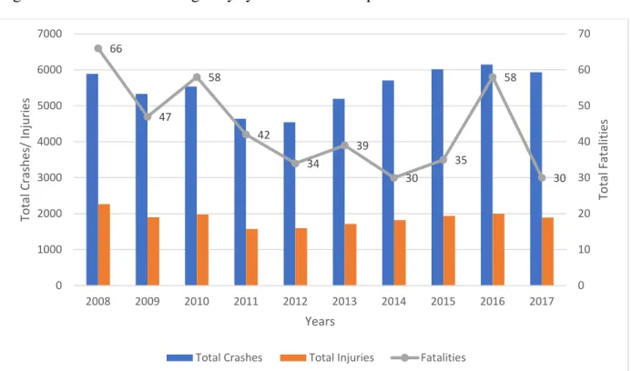
The state of Iowa serves as a major freight thoroughfare in the Midwestern United States, particularly along Interstate 80 and Interstate 35, which are major transport corridors serving east-to-west and south-to-north traffic, respectively. Figure 1-1 shows the layout of the Iowa Interstate network system. Besides, 80 and 35, other interstates include 235, 280, 380, I-480, I-680, I-29, and I-74. These routes cover a total length of 825 miles across the state. In addition to providing for efficient goods movement, another objective of the Iowa Department of Transportation (DOT) is to provide safe roadway conditions and facilitate progress toward the overarching goal of experiencing zero traffic fatalities. Figure 1-2 presents the history of crashes that have occurred on the Iowa interstate system from 2008 to 2017, including the numbers of total crashes and injuries, as well as the number of fatalities. It can be seen that fatalities have generally been decreasing while injuries and total crashes have largely plateaued. In order to facilitate further reductions in traffic crashes, injuries, and fatalities, an important objective is to allow for proactive design and the implementation of countermeasures that reduce the frequency and severity of crashes. One important tool in support of this objective is the use of safety performance functions (SPFs), which are mathematical models that can be used to predict the number of crashes that would be experienced for specific roadway geometry characteristics and traffic volumes.
Figure 1-1: Iowa Interstate highway system network map
Figure 1-2: Iowa Interstate crashes from 2008-2017 source from Iowa SAVER
These SPFs are provided in the Highway Safety Manual (HSM) (American Association
of State Highway and Transportation Officials (AASHTO), 2010), which provides guidance and best practices for safety management. The HSM is published by the American Association of State Highway and Transportation Officials (AASHTO). It provides analytical tools and
66 47 58 42 34 39 30 35 58 30 0 10 20 30 40 50 60 70 0 1000 2000 3000 4000 5000 6000 7000 2008 2009 2010 2011 2012 2013 2014 2015 2016 2017 To ta l Fa ta lit ie s To ta l C ra sh es / I nj ur ie s Years
techniques for quantifying the safety performance of various types of road facilities. The first edition of the HSM provides initially predictive methods for rural two-lane, two-way roads, rural multilane highways, and urban and suburban arterials. Subsequently, additional research has led to the development of SPFs for freeways and interchanges. These models were developed as a part of National Cooperative Highway Research Program (NCHRP) Project 17-45 and the content comprise supplementary Chapter 18 of the first edition of the HSM.
The primary data used for model calibration and validation were obtained from the Highway Safety Information System (HSIS) for the states of California, Maine, and Washington. It is important to note that research suggests the use of the SPFs from the HSM require local calibration or estimation of state-specific models in consideration of the fact that each state may have different features that are representative of the data from those three states. Concerns have been raised about the applicability, transferability, and accuracy of the SPFs. Studies of the calibration and development of jurisdiction-specific safety performance function were conducted
for Alabama, Utah, Oregon and Michigan(Brimley et al, 2012;Mehta and Lou, 2013;Dixon and
Avelar, 2015;Savolainen et al, 2015). A study in Utah developed new models for rural two-lane two-way highways and the results showed that the original HSM models under-predicted
crashes. Moreover, the study in Alabama developed state-specific statistical models for two-lane two-way rural roads, as well as four-lane divided highways and found that the
HSM-recommended method for calibration estimation performs well. A study to assess the
transferability of the HSM predictive method using data for a two-lane rural road network in the province of Salerno in Italy (Russo et. al, 2014). The results suggested that local safety
performance functions and crash modification factors (i.e. CMF) should be developed to more effectively implement the HSM techniques.
It is necessary to conduct state-specific SPFs and validate the HSM predictive methods. The HSM recommends each state to have its own SPFs, and the manual outlines three different ways for states to use and apply SPFs to make better decisions: (1) network screening to identify potential improvement; (2) determining effects of safety treatments or countermeasures; and (3) determining safety impacts of changed design on project level.
The Federal Highway Administration (FHWA) sponsored a project focused on
developing state-specific SPFs (Srinivasan, Bauer, 2013). The project report provides guidance on how to develop local SPFs. Various forms of nonlinear regression models were considered, including power, sigmoidal, and negative binomial functional forms. There are a few studies conducted the statistical model comparison, thus, based on a state-specific database, model selection may result in different coefficients when forming the SPFs which will be introduced under the literature review chapter.
Iowa generated its first version of Iowa DOT Data Driven Safety Guidance (Iowa
Department of Transportation (Iowa DOT) , 2017) in October 2017. The intent of the document is to provide guidance on safety analyses for Iowa DOT interchange projects. This guidance concerns CMFs for use in crash frequency prediction, based on information from the CMF clearinghouse. Calibration factors developed by Iowa DOT's Office of Traffic and Safety are included, which can be used to adjust the HSM SPFs to Iowa conditions. Table 1-1 provides segment calibration factors developed by the Iowa DOT for urban and rural freeway segments, as well as two-lane highway segments. These calibration factors represent the average rate by which the base models from the HSM tend to over- or under-estimate crashes of various types on Iowa highways. Calibration factors greater than one are reflective of cases where the HSM models under predict actual (observed) crashes based on Iowa data while calibration factors less
than one correspond to cases where the HSM models tend to over predict. At this moment, the Iowa DOT has not developed state-specific safety performance functions using data from Iowa. Table 1-1: Iowa SPF Segment Calibration Factors (Iowa Department of Transportation (Iowa DOT) , 2017)
Crash Type Calibration Factor
Urban Freeway
Multiple-Vehicle Fatal and Injury 1.26 Multiple-Vehicle Property Damage
Only 1.79
Single-Vehicle Fatal and Injury 0.85 Single-Vehicle Property Damage Only 1.17
Rural Freeway
Multiple-Vehicle Fatal and Injury 1.08 Multiple-Vehicle Property Damage
Only 1.67
Single-Vehicle Fatal and Injury 0.64 Single-Vehicle Property Damage Only 1.16
Rural, Primary, Two-Lane Road Segments
All crashes 0.84
1.2Research Objective
The initial objective of this study aims to see if follow the HSM predictive method, will the model well-transferred and suit Iowa data. With regards of this objective, a series of SPFs are developed. Negative binomial regression models were estimated, as recommended by the HSM. An Interstate database was assembled to examine the safety performance of the mainline system, wherein segments are comprised of uniform characteristics and are exclusive of interchange and ramp sections. Segments with lengths shorter than 0.1 miles were combined with adjacent segments in ArcMap, as the HSM suggests a minimum segment length of 0.1 miles. The final analysis database includes segment-level traffic information, geometric characteristics, and roadside data, along with crash counts during the analysis period from 2012 to 2016.
A series of SPFs were estimated using subsets of these data with the intent of validating the accuracy of the predictive models separately across space and time, as well as with respect to both dimensions. Goodness-of-fit is compared using metrics that include mean absolute error (MAE), mean squared error (MSE), root mean square error (RMSE). Ultimately, the results provide guidance as to the relative issues posed by temporal and spatial transferability.
1.3Thesis Structure
This thesis consists of six chapters in total. This introductory chapter provided the motivation for the present study. The remaining chapters are briefly described below:
• Chapter 1: Introduction- This chapter introduces the background on general
information related to the documentation of safety predictive method. The main reference is mentioned as well as the necessity of current research objective. The following sections under this chapter are stating the detail information of the research objective.
• Chapter 2: Literature Review- This chapter is structured into three parts to
summarize the existing papers established in the related area. This chapter begins by examining previous studies on a validation techniques that inspired the present study. Those techniques gave insights on how to compare and identify function performance, and how to assess transferability of models by focusing on data sample design. Additional work on analytic methods involving before-after and cross-sectional as well as Empirical Bayes are discussed. The second section examines state practices on SPFs development. The last section briefly
introduces the negative binomial model and talks about the applied examples in similar studies.
• Chapter 3: Data Description- This chapter describes the data used in this study, including databases from Iowa DOT and manually combined segments. A data integration process using ArcMap is presented. All variables used in data analyses are summarized statistically including crash data, traffic data and roadway characteristics.
• Chapter 4: Methodology- This chapter states the statistical methods and
validation techniques used in this study, including the general formulas, coefficient descriptions, and reasons for selecting those methods. A detailed study design is presented to talk through how to validate the model across time, space and both dimensions, and how to examine transferability by designing the sub-datasets.
• Chapter 5: Results and Discussion- This chapter presents the results of the
statistical models developed for this study under each validation purpose and examines why those results were obtained.
• Chapter 6: Conclusion and limitation- This chapter concludes this study with a
concise summary of key findings. Limitations and expectations for future work are presented.
CHAPTER 2. LITERATURE REVIEW
This chapter is organized into three sections to introduce previous work on safety model transferability. The first section introduces two study cases on applying validation techniques and comparing SPF models, which inspired the present study. The second section examines how various states have either developed their own SPFs or calibrated HSM predictive methods. The third part examines previous studies on the development of negative binomial models for safety performance prediction.
2.1 Validation technique and analytic method
There were two validation cases in recent years on safety performance functions which inspired the methodology of the present study. This research (Dixon and Avelar, 2015) applied a validation technique to safety performance functions developed by the Oregon DOT for arterial segments. The Oregon DOT previously developed its own SPFs for arterial segments, and the validation activities were assessed within three technique approaches: spatial transferability, spatial-temporal transferability, and individual coefficient stability and significance of the models.
To examine spatial transferability, the researchers reviewed the model results for the same year in the original analysis at a different group of sites. The direct comparison results are shown in Figure 2-1. The predicted values are not statistically different from the observed values because the p-value of goodness-of-fit (GOF) was 0.0828 but should at least equal to 0.05 when achieve a 95% confidence interval.
For the spatial-temporal transferability approach, the predictive power of the model was verified for a different time period. The sites were controlled, the spatial analysis was designed into two time-base cases: (1) only crashes occurring from 2009 to 2011; and (1) all crash data
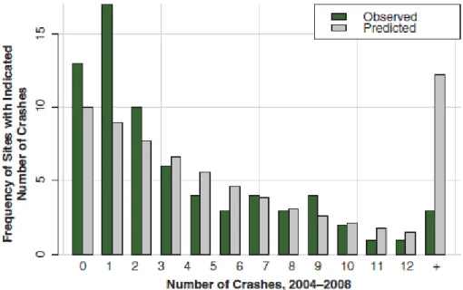
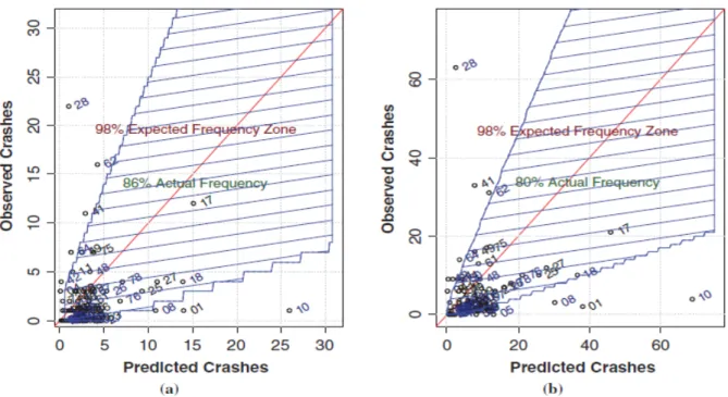
from 2004 to 2011. The direct comparison results are shown in Figure 2-2. The paper pointed out that it was reasonable to expect the variability of crash frequency to increase when the number of crashes increased. The authors constructed the plot to compare observed crashes versus predicted crashes graphically, as shown in Figure 2-3 and 2-4 respectively for the two time-base cases. The analysis indicated that the predictive power of the urban model was generally suitable, and the predictive model tended to deviate from the observed crash frequencies more than expected.
Figure 2-1: Original model predictions versus observed validation crashes (urban) p-value= 0.0828 (Dixon and Avelar, 2015)
Figure 2-2: Crash distributions associated with time for (a) 2009-2011 and (b) 2004-2011 (Dixon and Avelar, 2015)
Figure 2-3: Predicted and observed urban crash frequencies for 2004-2008 (sites are identified by a number) (Dixon and Avelar, 2015)
Figure 2-4: Site expected frequencies for (a) 2009-2011 and (b) 2004-2011 (Dixon and Avelar, 2015)
As noted in the final guidance report, temporal correlation could result in incorrect estimations of coefficients’ standard errors. The guidance provided methods for addressing this issue by estimating generalized equations or using random effect negative multinomial models (Srinivasan, Bauer, 2013).
Regarding the approach of equivalent model coefficients, the accuracy of coefficient values of the original model was analyzed and verified. In addition, a study examined the theoretical characteristics of the modeling approach and compared them using two different datasets. The results showed that these methods had very similar performance. A sensitivity analysis was conducted to explore how the performance of these techniques vary by degree of dispersion and observed correlation levels of total and severe injury crashes with potential explanatory variables (Avelar, Veronika, Jirˇí, 2018).
Another study validated FHWA crash models for rural intersections. The validation was conducted using internal validation and external validation approaches. Internal validation took
care of the underlying phenomenon explanation, and external validation was concerned with the temporal and spatial transferability of the predictive model. It also focused on GOF, using mean prediction bias, Mean Absolute Deviation (MAD), Mean Squared Prediction Error (MSPE) and Pearson product moment correlation coefficients between observed value and predicted values. The preliminary validation consisted of running models for different years for the same
intersection. This aimed to assess the ability of models to forecast crashes across time. Data from Minnesota was used to provide multiple years of accident data, and data from Georgia was used for model validation across jurisdictions. The external validation used GOF of the statistical models to compare independent data (Oh et al., 2003).
The NCHRP 17-45 report (Bonneson et al., 2012) provided a two-step process for model validation. The first step required predicting the crash frequency using calibrated models from a third database which was not utilized for the development of SPFs as known as the calibrated models. The second step required comparing CMFs between calibrated CMFs and similar CMFs mentioned in previous literature to ensure that the calibrated CMFs were consistent with
previous research results. As mentioned previously, data from three states were included in the HSIS database. The models were developed using data from California and Washington, with data from Marine excluded for validation purposes. A study came to reference which applied geographically weighted regressions to account for spatial heterogeneity to evaluate whether SPFs would vary across space. This study identified better performance between two different negative binomial regression models through the comparisons based-on time and space basis: (1) geographically weighted negative binomial regression and: (2) traditional negative binomial
regression. The log likelihood, Pseudo-R2 and AIC (Akaike Information Criterion) were used to
To validate models across time, the before-and-after method could be used, while cross-sectional study are commonly used for assessing space bias throughout samples. In addition, Empirical Bayes and full Bayes methodology are often used for road safety studies. An article (MacNab and Ying C., 2003) illustrated modelling technique implementation in accident and injury surveillance and prevention system which could be utilized by transportation or health agency to examine routine on accidents, injuries, and hospitalizations and target high-risk
regions. An empirical Bayes inference technique using penalized quasi-likelihood estimation was implemented to model both rates and counts, with spline smoothing accommodating non-linear temporal effects. The technique introduced in this article providing application and illustration on spatial-temporal modelling framework as part of accident surveillance and prevention system to identify the high-risk regions. A Bayesian hierarchical Poisson random effects spline model incorporated both spatial and temporal components into a unified framework to space and time surveillance. A validation study (Wang, Abdek-Aty, Lee, 2016) for a Full Bayes methodology for observational before-after studies was conducted and the results supported that the Full Bayes could provide similar results as Empirical Bayes. To examine SPFs’ transferability for
developing CMFs, a study modified before-after study with EB adjustment which was a method combining before-after and traditional EB to strengthen on case control techniques when using regression models. The paper pointed out that this combo method could make the estimations more precise and correct the bias of regression to mean.
In a word, the validation should be designed and conducted either across time or across space or both dimensions. A few studies were conducted using data from outside of the U.S. that to examine international transferability in other countries such like Italy and Canada (Russo et al., 2014; Martinelli et al., 2009; Persaud et al., 2012)
2.2 HSM predictive method calibration and state-specific SPFs examples
Researchers and state DOTs have been working on the calibration of HSM and developing customized SPFs. In 2010, a study (Garber, Haas, Gosse, 2010) examined SPFs provided by SafetyAnalyst, a software tool that provides SPFs for two-lane roads in Virginia but which was based on data from Ohio. The study developed separate models for urban and rural areas through generalized linear modeling with negative binomial distribution assumed crashes. The results indicated that the SPFs developed using local data fit better than the results obtained from SafetyAnalyst.
The state of Illinois completed a project and established a report (Robert, Jang, Ouyang, 2010) on development of state-specific SPFs. In this report, predicted SPFs were applied for roadway segments and intersections under Illinois DOT's jurisdiction by modeling the
relationship among traffic, geometric conditions and crash density. The developed SPFs were used to identify high potential locations for safety improvements. Florida also established a report (Srinivasan and Bauer, 2011) on developing and calibrating HSM predictive methods for Florida conditions both on segment-level and intersection-level. The study suggested that the models should be developed at a lower level to obtain better results, because district-level or population-group-level calibration factors tend to achieve more adequate results than state-level.
In 2012, two papers talked about development jurisdiction-specific SPFs both using negative binomial regression models. One was the city of Regina, Saskatchewan, using five-year crash data from 2005-2009 (Young and Park, 2012), and another was the State of Utah (Brimley et al., 2012). They both concluded that state-specific SPFs provided the best fit to the data.
In 2014, a research (Kweon, Lim, Turpin, Read, 2014) was conducted on a customized SPF development procedure for Virginia DOT by using empirical data on four-leg signalized intersections of rural multilane highways. Within the same year, another study (Islam, Ivan,
Lownes, Ammar, Rajasekaran, 2014) conducted SPFs development for Connecticut's Interstate highways separately on single-vehicle and multivehicle crashes. All geometric variables were used to estimate SPFs in form of negative binomial, and the best fit model was identified by comparing goodness-of-fit metrics. The results suggested that it was important to incorporate the interaction effect between the speed limit and geometric variables.
Internationally, SPFs calibrations were conducted based on HSM predictive method for urban four-lane divided roadway with angle parking in Riyadh, Saudi Arabia (Khalid and Mohamed, 2015). The study developed new SPFs using negative binomial regression models. The datasets contained fatal and injury crashes with AADT, geometric design feature data for undivided four-lane roadway (U4D) to calibrate HSM predictive method, and the resulted showed that the new SPFs performed better than the calibrated model in crash prediction.
Recently, Pennsylvania developed regionalized SPFs for two-lane rural roads by
modelling three regional levels: statewide, engineering district and individual countries. Negative binomial models were utilized to form the SPFs, the statewide database consisted of large size data more than 10,106 miles and over 113,600 reported crashes. Three methods were used to compare different regionalized SPFs using GOF, cumulative residuals plots, and RMSE. The predicted values were compared to observed values based on 8 years' data. The results indicated that the district-level SPFs with county-level adjustment factors had a better performance in predicting crashes than other regional SPFs. It was necessary to develop an analytical method which can combine the results of before-and- after studies with cross-sectional studies in a meaningful and useful way (Li, Gayah, Donnell., 2017; Oh et al., 2003).
2.3 Negative binomial model election
To develop state-specific safety performance functions, statistical models need to be considered. The HSM recommends using the negative binomial model to develop state-specific
safety performance functions. This section did provide a wide range reviews of paper relate to or involve negative binomial in studies.
Traditional Poisson and Poisson–gamma (or negative binomial) distributions were mentioned as the most common and popular statistical models for transportation safety analysts for modeling motor vehicle crashes (Srinivas and Dominique, 2008). There were some previous studies conducting the comparison between commonly used statistical models. When selecting models, their advantages and disadvantages should be known. For example, since panel data became available and popular in the safety area, heterogeneity may bias the results and the issue needs to be addressed. Study results (Karlaftis and Tarko, 1998; Ambros et al., 2016) indicated that significant differences existed among the developments of modeling. It was shown that separate models were more efficient than the joint model, and simple crash prediction models were found sufficient for network screening.
In 2007, a paper published on crash prediction model focusing on multilane rural roads in Italian. The Poisson, negative binomial and negative multinomial regression models were used to form the models and predicted the frequency of accident occurrence. Besides the common
variables, safety effects such as stopping sight distance and pavement surface characteristic were taken into consideration. Moreover, separately analysis models were developed for tangents and curves. Regarding the model comparison, negative multinomial distribution was suggested as the most appropriate statistical regression tool for longitudinal crash data analysis. Because both Poisson and negative binomial models required the accident data to be uncorrelated in time, the random effect negative binomial model became more suitable due to the unobserved
A different study evaluated the performance of Poisson and negative binomial regression models for analyzing the relationship between truck accidents and geometric design of road sections. The unknown parameters were estimated using the maximum likelihood method and results showed that negative binomial regression models using moment and regression-based methods should be used with caution (Miaou, 1994).
A similar study was conducted to examine impacts of roadway geometric features on rural two-lane highway crash severity using data from Illinois from 2007-2009. This analysis used standard ordered logit and multilevel ordered logit as statistical models. The results showed that the multilevel ordered logit model provided greater consistency with the data generating mechanism and could be utilized to evaluate the safety effects of geometric design improvement projects (Haghighi, Liu, Zhang, Porter, 2018).
Another study sought to document a new type of model, using the Generalized Waring (GW) distribution. The GW model could yield more information about the observed variance in
datasets by separating it into three parts: randomness (explaining the model’s uncertainty),
proneness (the internal differences between entities or observations), and liability (variance
caused by other external factors that are difficult to identify and which were not included as explanatory variables). The results showed that the GW model could provide meaningful information about the source of variance in crash data, and yielded a fit better than the negative binomial model for both empirical datasets (Peng, Lord, Zou, 2014).
A Bayesian hierarchical Poisson random effects spline model incorporated both spatial and temporal components into a unified framework for space and time surveillance. The tool might be used for routine monitoring focusing on visually describing the spatial distribution of accident rates/ratios over regions and time in order to link critical factors for further investigation
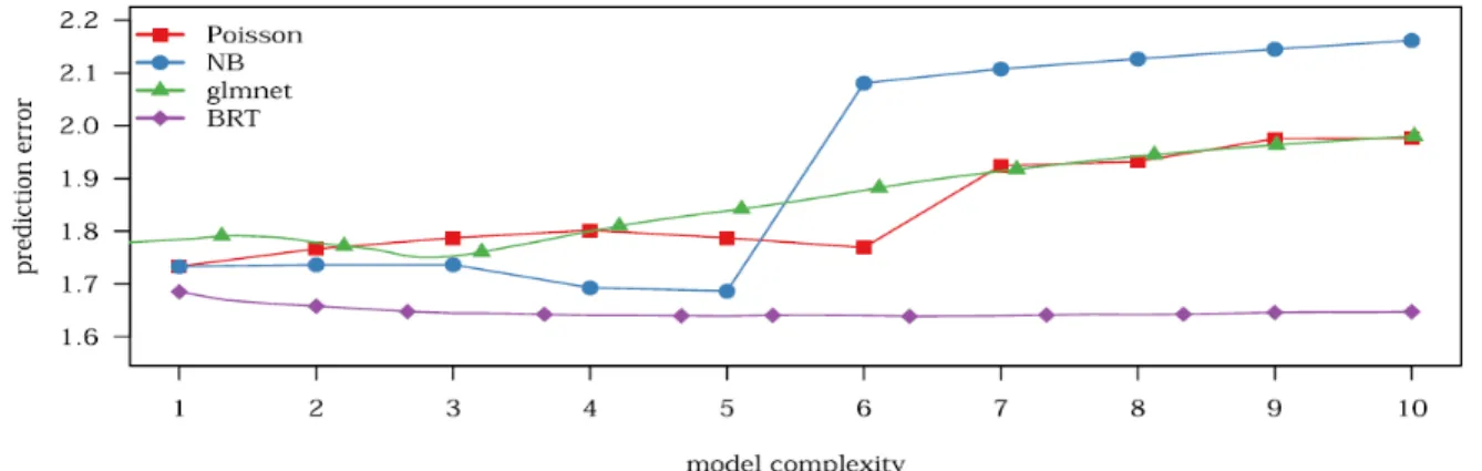
(MacNab and Ying C., 2003). A project (Wang et al., 2016) used 36 safety-related parameters for three- and four-legged non-signalized intersections in Alabama, aiming to explore the influence on intersection characteristic scores while choosing statistical models for estimating SPFs. Poisson regression, negative binomial regression, regularized generalized linear model (GLM) and boosted regression trees (BRT) were used to evaluate SPFs. The results are shown in Figure 2-5. The figure shows the error for each type of model at different levels of complexity. The BRT model had substantially lower prediction error and relatively stable performance than the other three models. The Poisson regression model is the one most used to generate SPFs, as it captures the discrete nature of count data. However, negative binomial was considered better than Poisson since count data is often overdispersed in Poisson models. The traditional GLM models form the linear structures which could only assign the importance to the linear relationship between some intersection characteristics and crash rate.
Figure 2-5 Cross-validated prediction error measured by the negative mean log-likelihood (Wang et al., 2016).
CHAPTER 3. DATA DESCRIPTION 3.1 Overview of Data Description
The main purpose of this study is to examine the spatial and temporal transferability of crash prediction models which are generated to obtain SPFs. The models were estimated using subsets of the data and a validation process was conducted to evaluate the predictive ability and performance of each model over space, time and both dimensions. Two databases were the primary source of data: the Geographic Information Management System (GIMS) database and the Iowa Crash database. GIMS contains traffic information as well as roadway geometric characteristics, and the Iowa Crash database compiles all reported crashes within the state of Iowa from police reports. Manual segment combination was conducted in order to achieve Highway Safety Manual (HSM) minimum segment length suggestion, and all involved segments' lengths were greater than 0.1 miles. ArcGIS and Microsoft Excel were used for data integration
3.2 Iowa DOT Geographic Information Management System
The Iowa DOT GIMS database contains georeferenced data describing numerous aspects of roadway information. The database is updated every other year to incorporate changes due to highway construction or maintenance activities. Each segment is assigned a link number called MSLINK which is an auto-incrementing variable assigned by the Modular GIS Environment software. MSLINK is the key reference for assembling and joining data in ArcGIS. There are 13 different datasets in GIMS that cover almost all information for a specific roadway segment location, such as traffic information, roadway geometric design characteristic, etc. Among those datasets, Traffic, Road Info, and Direct Lane were mainly utilized in this study.
The Traffic dataset provides information on traffic parameters, such as annual average daily traffic (AADT) and vehicle type distribution (i.e., the proportions of different classes of
vehicles in mixed traffic volume). The Road Info dataset contains geometric information of roadway segments including surface type/width, median type/width, lane numbers and types (i.e., through lanes, turning lanes, two-way left turn lanes, etc.), etc. The Direct Lane dataset gives various characteristics related to roadway infrastructure or countermeasures, such as posted speed limit, shoulder type/width, curb presence, rumble strip installation conditions, etc.
3.3 Iowa DOT Crash Database
The Iowa DOT crash database records all reported crashes occurring in the State of Iowa. There are three subsets at the person level, vehicle level, and crash level. The database provides the crash date, location, and manner of collision, weather/light condition, crash severity, first harmful event, crash types, driver age, sex, and other crash information, integrated from police reports. For this study, only the crash-level dataset was used.
Five years of crash data from 2012 to 2016 were integrated using ArcGIS and Microsoft Excel for this study. Crashes occurring along mainline Interstate highways (i.e., on through-lane sections) were identified and intercepted by applying a 50 feet buffer distance from the roadway mainline. QA/QC procedures were conducted to ensure the buffer width was selected correctly to contain relevant crashes.
3.4 Segment Combination
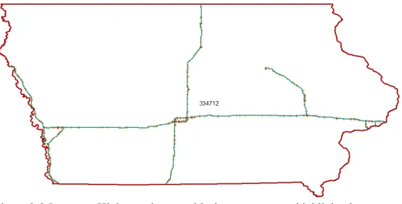
Loading GIMS geodatabase in ArcGIS, all segments under Iowa DOT jurisdiction could be filtered out by using ‘select by attribute’ and making queries ‘Justice=1.’ Figure 3-1 shows the overview roadway layout under Iowa DOT jurisdiction. In order to get the interstate mainline system, new queries were made through ‘select by attribute' function as ‘syscode=1’ (i.e. Interstate highway classification code), ‘NINEONEONE' involving RAMP, LOOP, ST, SPE CASE, US20, etc. to clean current layout and show interstate mainline system only. Besides using queries for filtering, a column indicating roadway function was used as an additional check. Further checking was conducted while was doing the segment combination. After preliminary assembly, there were 4,153 segments under the interstate system and each segment owned unique MSLINK. Of these, 2,109 segments were shorter than 0.1 miles, which could not be used in model analysis according to the HSM. In Figure 3-2 below, the Iowa interstate mainline system is shown and shorter segments which needed to be combined to nearest longer segment are highlighted in red.
Figure 3-2 Interstate Highways layout with shorter segments highlighted
Segment combination was conducted by adding a new column called ‘NewID’. The idea was to combine segments with lengths shorter than 0.1 miles to their nearest segments with lengths greater than 0.1. Manual combination was done because shorter segments were often located next to each other, making automated combination unreliable as engineering judgment was required to arrange the combination. After this process, the shorter segment’s MSLINK was changed to the MSLINK of the nearest longer segment under the NewID column, and the longer segment MSLINK remained the same. As mentioned previously, QA/QC was conducted during combination. Leftover ramp sections and very short isolated segments were removed. The final step of the combination used the ‘Dissolve’ function to spatially combine the segments based on NewID. New segment lengths were calculated for the combined segments. At the end of this process, there were 2050 segments with lengths ranging from 0.1 to 1.6 miles on the interstate mainline system.
3.5 Data Integration Process
With segment combination accomplished, roadway geometry, direct lane, and traffic info were joined to assemble a comprehensive database using the new segment definitions. Concerns
arose at this point that the geometric information used data from 2015 rather than individual geometric datasets for different years. For this study, an important assumption was made that the geometric information was consistent throughout the five-year period. The shorter segments were assumed to have the same characteristics with the nearest longer segments. For this study, the roadway and roadside features were all transferred into binary indicators for analysis. Crashes were spatially identified by making a 50ft buffer around the roadway centerlines as defined in the shapefiles. The 50-ft distance was determined from trial and error. Several
attempts were made using values from 20ft to 150ft to obtain interstate crashes without involving nearby crashes on local streets or ramp sections. A 50-ft distance achieved the best performance in this regard.
To export the attribute table from ArcGIS, some dataset restructuring and recoding was necessary. There were a few segments missing AADT data. To solve this issue, the AADT of the nearest segment was applied. This was done manually in ArcMap. During the column check, surface width, as well as median width, were excluded from analysis due to apparent
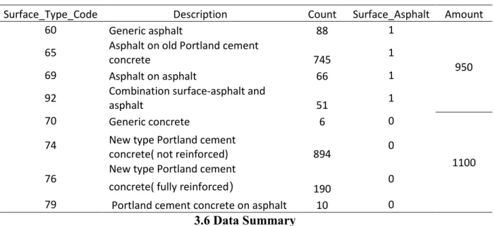
measurement bias. The surface width definition was not officially defined, while median width and surface width were confused when approaching interchange areas. Binary indicator variables would be used to minimize the bias. The surface type was recoded based on material (either asphalt or concrete), which is shown in Table 3-1. The median type was recoded into two binary categories which indicated whether a barrier installed or not, and whether the median surface was paved or grassy. The median barrier determination was made by comparison with Iowa DOT Cable Median Barrier Project Geodatabase records. Each column was checked before integration with the analysis tool; 42 out of 2050 records showed two lanes under the “number of lanes” column, but this did not match lane type records which had been corrected. Regarding the
lane number and lane type data, the new column called ‘Transition_zone’ was recoded which indicated current segment located within transition area (i.e. lane type record involves number 6_exit lane, 7_entrance lane, 9_other).
Table 3-1 Recoding summary for Surface_Type
Surface_Type_Code Description Count Surface_Asphalt Amount
60 Generic asphalt 88 1
950
65 Asphalt on old Portland cement concrete 745 1
69 Asphalt on asphalt 66 1
92 Combination surface-asphalt and asphalt 51 1
70 Generic concrete 6 0
1100
74 New type Portland cement
concrete( not reinforced) 894 0
76 New type Portland cement concrete( fully reinforced)
190 0
79 Portland cement concrete on asphalt 10 0
3.6 Data Summary
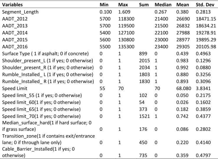
To obtain a better fit crash prediction model for a segment group, 10 different predictor variables were included to generate safety performance functions including segment length, AADT, and binary indictor variables covering surface type, and roadside/roadway features. Those variables could be used in SPFs to predict crash frequency. The descriptive statistics of the predictor variables are shown in Table 3-2. Segment lengths ranged from 0.10 to 1.61 miles, with a total length for all analysis segments of 779.97 miles. The presence of rumble strips, median features, and speed limits are treated as binary indicators in the models, following the HSM recommendations. In addition, each segment’s yearly crashes were counted. There were 2050 segments in the Interstate database, and 24,617 crashes were reported on Interstate segments from 2012 to 2016, as shown in Table 3-3.
Table 3-2 Interstate database descriptive statistic summary
Variables Min Max Sum Median Mean Std. Dev
Segment_Length 0.100 1.609 0.267 0.380 0.2813 AADT_2012 5700 118300 21400 26690 18471.15 AADT_2013 5700 119500 21500 26832 18634.21 AADT_2014 5400 127100 22100 27988 19278.91 AADT_2015 5600 130800 23000 28977 19895.29 AADT_2016 5500 135300 23400 29305 20105.98
Surface Type ( 1 if asphalt; 0 if concrete) 0 1 899 0 0.439 0.4963 Shoulder_present_L (1 if yes; 0 otherwise) 0 1 2015 1 0.983 0.1296 Shoulder_present_R (1 if yes; 0 otherwise) 0 1 2034 1 0.992 0.0880 Rumble_Installed_ L (1 if yes; 0 otherwise) 0 1 1803 1 0.880 0.3256 Rumble_Installed_ R (1 if yes; 0 otherwise) 0 1 1830 1 0.893 0.3096
Speed Limit 55 70 70 68.080 3.8341
Speed limit_55 (1 if yes; 0 otherwise) 0 1 102 0 0.050 0.2175 Speed limit_60(1 if yes; 0 otherwise) 0 1 54 0 0.026 0.1602 Speed limit_65(1 if yes; 0 otherwise) 0 1 373 0 0.182 0.3859 Speed limit_70(1 if yes; 0 otherwise) 0 1 1521 1 0.742 0.4377 Median_surface_hard(1 if hard surface; 0
if grass surface) 0 1 176 0 0.086 0.2802
Transition_zone(1 if contains exit/entrance
lane; 0 if through lane only) 0 1 450 0 0.220 0.4140
Cable_Barrier_Installed(1 if yes; 0
otherwise) 0 1 735 0 0.359 0.4797
Table 3-3: Crash data summary
Min Max Sum Median Mean SE.Mean CI.Mean.95% Std.Dev
Crash_2012 0 63 5578 1 2.721 0.0917 0.1798 4.1502
Crash_2013 0 60 5472 1.5 2.669 0.0853 0.1673 3.8618
Crash_2015 0 33 4693 1 2.289 0.0735 0.1442 3.3296
CHAPTER 4. METHODOLOGY
Under this section, the detailed methodology used as a part of this study is discussed, including a description of the statistical methods, validation techniques and goodness-of-fit tests. As the primary purpose of this study is to examine the spatial and temporal transferability of SPFs, a description of how the analysis datasets prepared is first presented.
4.1 Data Preparation and Summary
The full database described in the previous chapter is comprised of 2,050 segments. For each segment, geometry, traffic volume, and crash data are obtained for two-time periods: (1) 2012 to 2013; and (2) 2015 to 2016.
After the original database was developed, random selection was conducted in R studio. The original database was divided into two equal size subsets named Group_A and Group_B respectively. Ultimately, Group A and B from random selection used in this study had similar total segment length, and the differences among total crashes for each year were smallest. The descriptive summary of Group A and B can be found in Table 4-1. From the summary, the total length of segments of Group_A was 389.548 miles, and Group_B had similar total segment length as 390.424 miles. It could be seen that Group A and B had similar feature distributions. For example, the groups are well balanced with respect to traffic volumes, surface type, speed limit, and other geometric characteristics.
Table 4-1: Subset descriptive statistic summary
Group_A Group_B
Sum Mean Std.Dev Sum Mean Std.Dev
Segment_Length 389.548 0.38 0.28 390.424 0.38 0.29
Average AADT of 2012-2013 27389600 26721.56 18069.62 27470115 26800.11 19029.48
Average AADT of 2015-2016 29806950 29079.95 19369.29 29931800 29201.76 20561.03
Surface Type ( 1 if asphalt; 0
if concrete) 455 0.44 0.50 444 0.43 0.5 Shoulder_present_L (1 if yes; 0 otherwise) 1008 0.98 0.13 1007 0.98 0.13 Shoulder_present_R (1 if yes; 0 otherwise) 1016 0.99 0.09 1018 0.99 0.08 Rumble_Installed_ L (1 if yes; 0 otherwise) 912 0.89 0.31 891 0.87 0.34 Rumble_installed_R (1 if yes; 0 otherwise) 921 0.90 0.30 909 0.89 0.32
Speed limit_55 (1 if yes; 0
otherwise) 49 0.05 0.21 53 0.05 0.22
Speed limit_60(1 if yes; 0
otherwise) 20 0.02 0.14 34 0.03 0.18
Speed limit_65(1 if yes; 0
otherwise) 195 0.19 0.39 178 0.17 0.38
Speed limit_70(1 if yes; 0
otherwise) 761 0.74 0.44 760 0.74 0.44
Median_surface_hard(1 if hard surface; 0 if grass
surface) 78 0.08 0.27 98 0.1 0.29
Transition_zone(1 if contain deceleration/acceleration
lane; 0 if through lane only) 213 0.21 0.41 237 0.23 0.42 Cable_Barrier_Installed(1 if
yes; 0 otherwise) 387 0.38 0.49 348 0.34 0.47
Total Crash of 2012-2013 5457 5.32 7.64 5593 5.46 7.56
Total Crash of 2015-2016 4184 4.08 5.62 4259 4.16 5.96
4.2 Statistical methodology of SPF development
Safety Performance Functions are crash prediction models developed from past observed crash data, site characteristics, and roadway traffic information. For developing
segment-level SPFs, the total crashes for analysis period would be used as the exposure variable. In this study, negative binomial regression model was run in R studio to obtain the SPFs, the accuracy and transferability of the models was examined.
4.2.1 Generalized Linear models
Crashes are randomly occurring events; crash data is nonnegative and discrete in nature. Consequently, some segments have minimal or zero crashes. This means that crash
distributions do not follow the normal distribution. In this case, in NCHRP 17-45, the researchers used nonlinear regression to develop SPFs. The traditional generalized linear models (GLM) models form the linear structures which assign the importance to the linear relationship between roadway characteristics and crash rates, and the models allow the predictor variables to have error distributions other than normal distributions. Also, the models can fit maximizing the likelihood or log-likelihood of the observed parameters
In a generalized linear model, the dependent variable Y is assumed to be generated from a specific distribution: usually either the normal, binomial, Poisson or Gamma distributions
are used. The distribution of mean, μ, depends on the independent variables, Xi. The
equation can be written as:
𝑃𝑃(𝑦𝑦𝑖𝑖) =𝜇𝜇𝑖𝑖 =𝑔𝑔−1∗(𝛽𝛽𝑖𝑖𝑋𝑋𝑖𝑖) (3)
Where 𝑃𝑃(𝑦𝑦𝑖𝑖) is the expected value, 𝛽𝛽𝑖𝑖𝑋𝑋𝑖𝑖 is the linear predictor, and g is the link function. Under this framework, the variable can be expressed as:
𝑉𝑉𝑉𝑉𝑉𝑉(𝑦𝑦𝑖𝑖) =𝑉𝑉(𝜇𝜇) =𝑉𝑉�𝑔𝑔−1(𝛽𝛽𝑋𝑋)� (4)
4.2.2 Negative Binomial Regression Models
There are two types of commonly used count models. As mentioned previously these are the Poisson and negative binomial (also known as Poisson-gamma models)
regression models. The negative binomial regression is a type of generalized linear
model where the dependent variable Y is count data for events occurring within a
defined time period. The probability of the number of crashes occurring within dataset during a specific time period is given by:
𝑝𝑝(𝑦𝑦𝑖𝑖) =𝑃𝑃(𝑌𝑌= 𝑦𝑦𝑖𝑖) =𝑒𝑒
−𝜆𝜆∗𝜆𝜆 𝑖𝑖𝑦𝑦𝑖𝑖
𝑦𝑦𝑖𝑖! (5)
where y𝑖𝑖is the number of crashes for segment i, and λi is the Poisson parameter for segment
i. For this study, λi will be the expected number of crashes at segment i for a given time
period. The expected number of crashes can be expressed as:
λ𝑖𝑖 = EXP(β1X1 + β2X2 + ⋯ + β𝑛𝑛X𝑛𝑛) (6)
where X1 through Xn are explanatory variables which represent site characteristics such as
traffic volumes, speed limit, roadside and cross-section features; β1 through βn are the
estimate coefficients obtained from the regression analysis. The mean number of crashes was assumed to be equal to the variance. However crashes occurred randomly, and crash data in nature therefore naturally have greater variances. This is known as overdispersion.
Overdispersion can be handled by adding an additional term to the expression for λi, as
shown below:
𝜆𝜆𝑖𝑖 =𝐸𝐸𝑋𝑋𝑃𝑃(β1X1 + β2X2 + ⋯ + β𝑛𝑛X𝑛𝑛 +𝜀𝜀𝑖𝑖) (7)
Here, the new term 𝜀𝜀𝑖𝑖is a gamma-distributed error term with a mean equal to one and
variance α (also known as the overdispersion parameter). The inclusion of the
overdispersion parameter allows the variance to differ from the mean, as demonstrated in the equation below:
This can be interpreted as follows. A positive estimated coefficient represents an increased effect in the total number of crashes, while a negative sign indicates a decreased effect in the total number of crashes. To obtain the marginal effect which represents the percentage increase or decrease in the number of total crashes, the equation can be expressed as:
∆𝜆𝜆= 100∗ �𝑒𝑒𝛽𝛽𝑛𝑛𝑋𝑋𝑛𝑛 −1� (9)
Where Δλ is the percentage change in the number of crashes.
4.3 Validation study design procedure and methods
Eight statistical models were developed using the negative binomial regression in R studio to fully examine the transferability of SPFs. Cross-validation was conducted using the results from those eight models and a validation technique was applied to examine the spatial and temporal transferability of SPFs as well as the predictive abilities.
The transferability of a model refers to the degree to transfer the results can be generalized from a research setting to other contexts or settings (Trochim, 2006). In this case study, negative binomial regression is used to develop local SPFs and examine whether the method could be transferred and fit well to Iowa data as recommended by the HSM. The transferability is examined across space, time and both dimensions.
Ultimately, eight models were developed, including four simple models (i.e. using a subset of available variables) and four full models (i.e. containing all significant variables). The models were developed using two data subsets, Group_A and Group_B, during different
analyzed time periods: 2012-2013 and 2015-2016. Four parts of these two subsets were used to develop SPFs and the results were utilized further to examine spatial and temporal
• Group_A during 2012-2013( Group_A1213)
• Group_A during 2015-2016( Group_A1516)
• Group_B during 2012-2013( Group_B1213)
• Group_B during 2015-2016( Group_A1516)
The models were then used to develop SPFs. For each of these four cohorts, a “simple” and a “full” model were generated, making eight models in total. These are referred to as, for
example, SPF_A1213_simple and SPF_A1213_full respectively representing the simple and full models
for Group_A1213 data.
The transferability was examined among the models as well as across the models. SPFs developed using same subset were compared to each other by goodness-of-fit statistics to assess how well the model fit the data. The predictive ability and accuracy of prediction were evaluated by applying the SPFs to different validation sites. These sites were excluded from the model development. Next, the predicted values were directly compared to the actual observed values. The validation approaches are introduced subsequently and summarized in Table 4-2.
To examine the spatial transferability, the locations were changed. SPF_A1213_simple and
SPF_A1213_full were applied to Group_B1213 data, while, SPF_B1516_simple and SPF_B1516_full were
applied to Group_A1516 data. Under this experiment design, the predictive ability across space
was assessed. Group A and B contain mutually exclusive groups of roadway segments randomly selected from the full segment set. The time periods used for developing SPFs and validation were the same (2012-2013 or 2015-2016).
To examine the temporal transferability, models developed under the earlier time series
were applied to the later time series. Under this approach, SPF_A1213_simple and SPF_A1213_full
SPF_B1213_full were applied to Group_B1516 data. Thus, the locations were the same but the time
periods were changed. The SPFs were developed using data from 2012-2013 and used to predict crashes expected to occur in year 2015-2016.
Spatial-temporal transferability was also examined using cross
validation.SPF_A1516_simple and SPF_A1516_full were used to predict the crash frequency of
Group_B1213 data; SPF_B1516_simple and SPF_B1516_full were applied to Group_A1213 data. This
approach controlled the location and time period at the same time to examine the model performance using completely different datasets across both time and space. This is the most common situation encountered when using the HSM method for local SPF development. Table 4-2: Transferability examination study approach design summary
Spatial transferability
SPFs developed data Validated data Model type
Group_A during 2012-2013 Group_B during 2012-2013 Simple Group_A during 2012-2013 Group_B during 2012-2013 Full Group_B during 2015-2016 Group_A during 2015-2016 Simple Group_B during 2015-2016 Group_A during 2015-2016 Full
Temporal transferability
Group_A during 2012-2013 Group_A during 2015-2016 Simple Group_A during 2012-2013 Group_A during 2015-2016 Full Group_B during 2012-2013 Group_B during 2015-2016 Simple Group_B during 2012-2013 Group_B during 2015-2016 Full
Spatial-temporal transferability
Group_A during 2015-2016 Group_B during 2012-2013 Simple Group_A during 2015-2016 Group_B during 2012-2013 Full Group_B during 2015-2016 Group_A during 2012-2013 Simple Group_B during 2015-2016 Group_A during 2012-2013 Full
This experiment design excludes the year 2014. On one hand, traffic information from 2017 was missing, so only five years of data could be obtained for this case study. On the other
hand, considering the nature of SPF, when SPFs were generated using two-year periods of crash count data, the units would be crashes per mile per two years.
As recommended by the HSM, the standard form of an SPF for roadway segments can be expressed using one of the three following forms (American Association of State Highway and Transportation Officials (AASHTO), 2010) (Srinivasan et al., 2011):
𝑁𝑁𝑆𝑆𝑆𝑆𝑆𝑆 =𝐿𝐿 ∗ 𝑒𝑒𝑎𝑎+𝑏𝑏∗ln (𝐴𝐴𝐴𝐴𝐴𝐴𝐴𝐴)
𝑁𝑁𝑆𝑆𝑆𝑆𝑆𝑆 =𝑒𝑒𝑎𝑎+𝑏𝑏∗ln(𝐴𝐴𝐴𝐴𝐴𝐴𝐴𝐴)+ln (𝐿𝐿)
𝑁𝑁𝑆𝑆𝑆𝑆𝑆𝑆 = 𝑒𝑒𝑎𝑎+𝑏𝑏∗ln(𝐴𝐴𝐴𝐴𝐴𝐴𝐴𝐴)+𝑐𝑐∗ln (𝐿𝐿)
It can be expected that driving on longer segments results in longer exposure time than the shorter segment. In this case, the number of crashes can be expected to increase while driving on the roadway. Therefore, the third equation was an adjusted form of SPFs which was suggested in the study received acknowledge from transportation professionals where a and b are regression coefficients to be estimated using crash data, c is a parameter indicating the relationship between crash frequency and segment length. In this study, the length of the segment had been offset in log form, which meant that the crash frequency was predicted as crashes occurred on unit mile which was crash per mile per analyzed year period, and the equations can be simplified as follow:
Simple model:𝑁𝑁𝑆𝑆𝑆𝑆𝑆𝑆 =𝑒𝑒𝑎𝑎+𝑏𝑏∗ln(𝐴𝐴𝐴𝐴𝐴𝐴𝐴𝐴) (10) Full model:𝑁𝑁𝑆𝑆𝑆𝑆𝑆𝑆 = 𝐸𝐸𝐸𝐸𝑝𝑝(𝑉𝑉+𝑏𝑏 ∗ 𝑙𝑙𝑙𝑙(𝐴𝐴𝐴𝐴𝐴𝐴𝐴𝐴) +∑ 𝑐𝑐∇𝑖𝑖 𝑖𝑖 ∗ 𝐸𝐸𝑖𝑖) (11) where ci is the parameter estimate for variable xi.
Goodness-of-fit measures are used to evaluate the ability of the models to represent the
observed data. McFadden’s pseudo R2 was used that the intercept model’s log likelihood was
When comparing models on the same data, the McFadden R2 would be higher for the model with
the greater log likelihood. The likelihood is the occurrence probability resulted in given
parameter estimates. The higher the likelihood is, the better the model. The Akaike Information Criterion (AIC) was used to evaluate the suitability of the models using the maximum likelihood concept. AIC describes the trade-off between variance and bias, and is calculated by:
AIC = –2LL +2 × NP (12)
where NP is the number of parameters. The lower the AIC value, the better the model is because
the number of parameters is a factor affecting the AIC, and effectively discourages overfitting of data by penalizing the addition of parameters. So the AIC can be used for comparing models with the same number of variables.
Because the analyzed facility was an Interstate highway system, the estimated models in this study may not capture the features as accurately as possible. In this case, simple model was necessary because the inclusion of more variables may increase the prediction errors. Previous studies suggest that simple models could be more effective for prediction. Better fit models were
identified by seeking smaller AIC, higher McFadden R2, and higher log likelihood.
Cross-validation is the process for out-of-example evaluation which can assess how the fit of a statistical analysis developed based on the independent dataset. The predictive accuracy of each model would be evaluated. In order to assess how good a prediction is that can be either measure the predictive accuracy per se or compare various predicted models. The process can validate the models through analyze the goodness of fit of the regression, check regression residuals, and check the predictive performance of models by being applied on the data which is not used in model development.
Mean absolute error (MAE) is a measure of difference between two continuous variables.
It is an average of the absolute errors where 𝜇𝜇𝑖𝑖 is the actual observed crash count and yi is the
predicted value from developed SPFs. The equation is:
𝑀𝑀𝐴𝐴𝐸𝐸 =∑𝑛𝑛𝑖𝑖=1|𝜇𝜇𝑙𝑙𝑖𝑖 − 𝑦𝑦𝑖𝑖|
Mean square error (MSE) is probably the most commonly used error metric. It penalizes larger errors because squaring larger numbers has a greater impact than squaring smaller numbers. The MSE is the sum of the squared errors divided by the number of observations. The equation is:
𝑀𝑀𝑀𝑀𝐸𝐸 =∑𝑛𝑛𝑖𝑖=1(𝜇𝜇̂𝑙𝑙𝑖𝑖 − 𝑦𝑦𝑖𝑖)2
The Root Mean Square Error (RMSE) is simply the square root of the MSE.
These three metrics can be used for model validation. The MAE measures the average magnitude of the errors in a set of predictions, and it is the average over the test sample of the absolute differences between prediction and actual observed crash count where all individual differences have equal weight. The MSE is a measure of how close the predicted value fit the actual observed data. The smaller the MSE, the closer the fit is to the observed data. Additional, RMSE is the square root of the MSE which can be expressed as the average distance of a data point from the fitted point measuring along vertical axis. Both metrics can range from zero to infinite and the direction of errors are different. They ate negatively-oriented scores, which means the lower values are better.
CHAPTER 5. RESULTS AND DISCUSSION 5.1 Model results of developed SPFs
To examine the transferability of safety performance functions, SPFs first needed to be developed. As mentioned in the previous chapter, four “simple” SPFs were generated using SPFs which included only AADT and segment length as their variables. Four “full” SPFs were developed by including all of the significant variables. In this study, variables achieved at least 95% confidence were retained in the SPFs.
Table 5-1 and 5-2 show the model results using Group_A1213. Treating segment length as
offset, the units of were crashes per mile per analysis period. The estimated number of crashes
from SPF_A1213_simple was higher than SPF_A1213_full. The simple model showed that the crashes
would increase by 1.36% if AADT increased by 1.0% and the full model presented an increase of 1.08% if AADT increased by 1.0%. When treating length as offset, the estimates of log (AADT) are generally close to 1, but the simple model had slightly higher estimates on log (AADT) and the full model estimate of log (AADT) was dropped within general range usually closed to 1.0. This was reasonable given that that simple model only includes length and AADT, and the full model contained all other potential variables which would tend to weaken and distribute the effect of AADT. In the full model, speed limit at 55 mph and 65 mph had positive estimates compared to the base condition with speed limit at 70 mph. The positive estimates indicated that those variables would increase the crash frequency. Since this study did not separate urban and rural areas, the results more likely implied the effect of the area where the segments were located. Urban areas usually have speed limits below 70 mph (a posted speed limit of 55 mph is common). Variables regarding asphalt surface and hard median also indicated urban locations, higher volume demand and more complex traffic transit situations resulting in
higher crash frequency. In addition, segments with cable median barriers had positive value of coefficient estimates which indicated those segments had higher crash frequencies. Cable median barriers were installed on those segments as a countermeasure to decrease crash severity, and drivers driving on those segments with cable median barriers installed were more likely to occur
crashes. To identify the better fit model between these two models, the higher McFadden R2 of
0.163, and the higher values of log-likelihood and lower AIC indicate that the full model performs better than the simple model.
Table 5-1: Model results using Group_A1213
SPF_A1213_simple
Coefficients: Estimate Std. Error Z value Pr(>|z|)
(Intercept) -11.249 0.44836 -25.09 <2e-16 *** log(Ave_AADT_1213) 1.36425 0.04391 31.07 <2e-16 *** --- AIC 4806.5 Std.Err 0.268 Theta 3.229 McFadden R^2 0.150934 2 x log-likelihood -4800.52 SPF_A1213_full
Coefficients: Estimate Std. Error z value Pr(>|z|)
(Intercept) -8.8128 0.73787 -11.94 < 2e-16 ***
log(Ave_AADT_1213) 1.08255 0.07248 14.936 < 2e-16 ***
Speed limit_55 0.73308 0.11559 6.342 2.27E-10 ***
Speed limit_60 0.34223 0.18001 1.901 0.057275 .
Speed limit_65 0.25781 0.0721 3.576 0.000349 ***
Speed limit_70 (base condition) N/A N/A N/A N/A
Surface_Asphalt 0.16571 0.04947 3.35 0.000809 *** Rumble_installed_R 0.19655 0.14411 1.364 0.172593 Rumble_installed_L 0.03747 0.1446 0.259 0.795558 Shoulder_present_R -0.16185 0.26717 -0.606 0.544637 Shoulder_present_L 0.05065 0.21714 0.233 0.815572 Cable_barrier_Installed 0.19147 0.06174 3.101 0.001928 ** Median_surface_hard 0.29576 0.11712 2.525 0.01156 * Transition_zone 0.12148 0.06284 1.933 0.053241 . ---
Table 5-2: Model results using Group_A1213 (Continued)
AIC 4759 Std.Err 0.329
Theta 3.729 McFadden R^2 0.163234
2 x log-likelihood -4730.98
*p<0.05, **p<.01, ***p<.001
SPF_A1516_simple and SPF_A1516_full are presented in Table 5-3. In addition to the variables
mentioned previously such as speed limit at 55 mph and 65 mph, asphalt surface and concrete median surface were associated with higher crash frequency. Cable median barrier installation was also associated with higher crash frequency. Right side rumble strip installation was captured with a positive estimate, implying that they also have an increasing effect on crash frequency. The rumble strips installed along the edges of the roadway can inform fatigued or distracted drivers when they are about to leave the travel lanes. The positive estimate here is still reasonable, since drivers on those particular segments are more likely to drive off the roadway, and rumble strips were installed as a countermeasure. Within these two models, the full model still had better performance with better GOF results. Recall the database was assembled at segment level, and geometric features were assumed unchanged throughout analyzed five years.
SPF_A1213 and SPF_A1516 all used Group_A data and this meant the sample size of these four
models were the same, and changed variables were average AADT values and actual crashes
observed on those segments. The McFadden R2 values for the 2015-2016 models are similar to
the 2012-2013 models, but the AIC and log-likelihood of SPF_A1516_full was much higher than
model SPF_A1213_full. The model results were different because of the model complexity as well