DOCUMENTOS DE TRABAJO
BILTOKI
Facultad de Ciencias Econ ´omicas. Avda. Lehendakari Aguirre, 83
48015 BILBAO.
D.T. 2007.04
Reconstructing Chi-squared Intra-table Distances
in the Analysis of a Set of Contingency Tables.
Documento de Trabajo BILTOKI DT2007.04
Editado por el Departamento de Econom´ıa Aplicada III (Econometr´ıa y Estad´ıstica) de la Universidad del Pa´ıs Vasco.
Dep´osito Legal No.: BI-2350-07 ISSN: 1134-8984
Reconstructing Chi-squared Intra-table Distances in the
Analysis of a Set of Contingency Tables
Z´arraga, A. and Goitisolo, B.
Departamento de Econom´ıa Aplicada III,
Universidad del Pa´ıs Vasco-Euskal Herriko Unibertsitatea
Bilbao, Espa˜na
[email protected] and [email protected]
6th July 2007
Abstract
To study similarities among the set of rows -and columns- of a contingency table, Correspondence Analysis usesχ2distances between row profiles -and column profiles- of that table. This article presents a factor analysis for the study of a set of contingency tables in which, unlike more classical methods such as the analysis of juxtaposition and Intra Analysis; the existing relationships within each table -defined across the χ2 distances-, are not altered.
Key wordsContingency tables, Simultaneous Analysis, Correspondence Analysis, Chi-squared distance
1
Introduction
The study of the relationships between two qualitative variables is frequently carried out by means of Correspondence Analysis of the associated contingency table. The principal characteristics of this analysis include the transformation of the information into relative frequencies; the concept of row (or column) profile of the contingency table; the use of a weighting applied to each profile and the definition of the χ2 distance between two profiles.
The use of thisχ2 distance guarantees the property known as the “principle of distributional
equivalence” (Benz´ecri & collaborateurs (1973), among others). This property allows us to add up two modalities of the same variable with identical profiles into a new modality weighted with the sum of their masses. This property is fundamental because it guarantees a certain stability of the results in regard to the definition chosen for the modalities of the variable.
On the other hand, the use ofχ2 distance allows us to study the relationship between the two
variables by analysing the difference between the frequencies of the contingency table and the expected frequencies under the hypothesis of independence; that is to say, except for a factor of scale, the well-known Pearson chi-squared (χ2) statistic. The aim of Correspondence
Analysis (Escofier & Pag`es 1998) is to decompose into its elements this relationship between two variables into a sum (or overlapping) of simple and interpretable trends and to measure their relative importance in order to sort them.
Therefore, in the simultaneous study of several contingency tables presented in this work special care has been put into not changing this χ2 distance between profiles within each
table.
After an overview of some of the concepts of Correspondence Analysis (§ 2), several contin-gency tables are analysed (§3), showing how the distances between profiles are altered when either of the two most frequently used methods is carried out: analysis of the juxtaposition of the tables and Intra Analysis. Next, Simultaneous Analysis and its characteristics (§ 4) are shown. In particular it is shown how the distances studied in this new method of anal-ysis fit the χ2 distances between two profiles when their corresponding contingency table is
analyzed separately. The practical importance of maintaining the within-tableχ2 distances
is shown in§ 10 by means of an example with real data where it is shown how the proposed Simultaneous Analysis, unlike juxtaposition or Intra Analysis, allows the existing structure in each table to be maintained.
2
Correspondence Analysis
Let I ={1, . . . , i, . . . , I} and J = {1, . . . , j, . . . , J} be respectively the set of rows and the set of columns of a contingency table that correspond to the modalities of two qualitative variables. Let kij denote the number of observations that possess the modality i ∈ I of
the first variable and the modality j ∈ J of the second variable, ki. =
P
P
i∈Ikij the associated margins and k =
P
j∈J k.j =
P
i∈Iki. the grand total of the table. Contingency tables are frequently transformed into relative frequency tables, obtained by dividing each elementkij by the grand total of the table. In this way, fij denotes the relative
frequency of possessing the modalities i and j of the first and second variables respectively and fi. and f.j the associated margins.
Each modalityj, j ∈ J, is associated with a column profile,{fij/f.j| i∈ I}and a weight,
f.j, is assigned to it. The set of column profiles constitutes the cloud of column profiles,
which can be represented in the space RI.
The degree of disparity between two column-profiles (j and j0) is measured by the so-called χ2 distance, which is computed as follows:
d2(j, j0) = X i∈I 1 fi. µ fij f.j − fij0 f.j0 ¶2 = = X i∈I k ki. µ kij k.j − kij0 k.j0 ¶2 (1) The coefficients 1/fi. weight the differences in calculating the distance between rows. These
weights are put in a diagonal matrix that determines the metric inRI.
Correspondence Analysis (Benz´ecri & collaborateurs 1973) aims to visualize the above men-tioned similarities by projecting the profiles on planes. These planes have to be such that they minimize the deformations that projection implies. The first step is therefore to look for the one-dimensional subspace H (figure 1) that maximizes the weighted sum of squares of the distances between the projections on H of all the couples of column profiles (j, j0):
MaxH X j∈J X j0∈J f.jf.j0 d2H(j, j0) = = X j∈J X j0∈J f.jf.j0 d2(hj, h0j)
This criterion is equivalent to the following: MaxH X j∈J f.j d2H(j, G) = = X j∈J f.j d2(hj, G)
where G is the centre of gravity of the cloud, that is to say, the point of coordinates fi,
i∈ I (figure 2). Each of the elements of that sum is known as a projected inertia of the column profile; so the criterion consists of maximizing the inertia projected by the set of all the column profiles. These criteria are, in turn, equivalent to the following least-square criterion:
MinX
j∈J
where the weighted sum of squares of the distances between the column profiles and their projections is minimized. ³³³³ ³³³³ ³³³³ ³³³³1 -6 C C C © © © C CC j0 j hj0 hj 0 H RI Figure 1: ³³³³ ³³³³ ³³³³ ³³³³1 -6 C C C j hj ´´ ´´ ´´ ´´´ 0 H RI Figure 2:
In any contingency table rows and columns play symmetrical roles, so by interchanging the subscripts i and j the analysis of the rows would be obtained.
In correspondence analysis there are also relations between the projections of the column profiles and of the row profiles, called transition relations, which allow us to study the association between the two sets of modalities.
3
Analysis of a set of contingency tables: Effect on the
χ
2distances
Let G = {1, . . . , g, . . . , G} be the set of contingency tables to be analysed. Each of them classifies the answers of k..g individuals to two qualitative variables codified in modalities.
All the tables have one of the variables in common (whose modalities, I ={1, . . . , i, . . . , I}, are the rows). The other variable of each contingency table can be different or the same, codified in the same or a different form. The modalities of the second variable in each table are Jg ={1, . . . , j, . . . , Jg}. On juxtaposing all these contingency tables, a joint set of
columnsJ ={1, . . . , j, . . . , J} is obtained.
The element kijg corresponds to the total number of individuals who choose simultaneously
table g ∈ G).
Moreover, as usual, the sum is denoted by a point on the corresponding element, that is to say: ki.g = X j∈Jg kijg ki.. = X g∈G X j∈J kijg k.jg = X i∈I kijg k..g = X j∈J X i∈I kijg k = X g∈G X j∈J X i∈I kijg
3.1
Analysis of a table
If we want to analyze the similarities among the set of columns of only one of this set of con-tingency tables separately, for example that of indexg, the column profile{kijg/k.jg| i∈ I}
will be considered in the spaceRI endowed with the metric of associated matrixk
..g/ki.g and
endowed with a weightk.jg/k..g. In this way, theχ2 distance between two column profiles is:
d2(j, j0) = X i∈I k..g ki.g µ kijg k.jg − kij0g k.j0g ¶2 (2) which distance is equal to that obtained in (1).
3.2
Analysis of the juxtaposition
For purposes of analysis, the juxtaposition of the set of contingency tables is considered to be a table. This implies transforming the table into relative frequencies by dividing each of its elements by the grand total.
fijg =
kijg
k The margins of this table are:
fi.. =
ki..
k f.jg =
k.jg
k
In this way, the column profile of the modality j of table g is{kijg/k.jg| i∈ I}. It is equal
to the profile obtained in the separate analysis of tableg. Nevertheless, the distance between two column profiles j and j0 of the same table g is:
d2(j, j0) = X i∈I 1 fi.. µ fijg f.jg −fij0g f.j0g ¶2 = = X i∈I k ki.. µ kijg k.jg −kij0g k.j0g ¶2 (3)
It can be shown that this distance does not coincide with that obtained in the separate analysis (equation 2) due to the fact that the metric of the space is now k/ki.., that is to
say, the inverse of the margin of the juxtaposed table instead of the inverse of the margin of table g (k..g/ki.g).
3.3
Intra-Table Analysis
In the analysis of the juxtaposed table the total inertia can be decomposed into between and within table inertia; or between and within equivalent column inertia, when all the tables possess the same modalities in columns. The aim of Intra Analysis (Escofier & Pag`es 1998) is to study the within inertia of the juxtaposed table. The elimination of between table inertia implies transforming the elements of the table into:
kijg−
ki.g k.jg
k..g
+ki.. k.jg k or expressing them in terms of relative frequencies:
fijg−
fi.g f.jg
f..g
+fi.. f.jg
With this transformation the column profilej, since the margins of the table are maintained with regard to the juxtaposition, turns out to be:
½ fijg f.jg − fi.g f..g +fi..| i∈ I ¾
and, in terms of absolute frequencies:
½ kijg k.jg − ki.g k..g +ki.. k | i∈ I ¾
As intended, the χ2 distance between two profiles j and j0 of the same table is equal to the distance between column profiles of the same table obtained in the juxtaposition analysis (equation 3). Therefore, since a metric based on the set of the tables is used, theχ2 distance
between column profiles of each separate table (equation 1) is not maintained.
4
Simultaneous Analysis
Simultaneous Analysis seeks to analyze several contingency tables jointly without changing the χ2 distances between the row profiles and column profiles of each table; in such a way
We will now briefly present the method, which can be found in detail in Z´arraga & Goitisolo (2002) and (2006) and will demonstrate in§8 how the factors obtained allow us to reconstruct the χ2 distances between the row or column profiles of each table.
The first step in maintaining the χ2 distances between two profiles (row or column) of each
table separately is to use the relative frequencies of each table, that is to say, to divide every element kijg by the grand total of the table g (k..g) and not by the grand total of the whole
of the G tables (k). This relative frequency will be denoted by fijg, that is to say: fijg = kijg
k..g
6
= kijg
k =fijg
This paper will also include the weight αg, used in Z´arraga & Goitisolo (2002). This weight
balances the influence of each of theGtables in the joint analysis in a similar way to Multiple Factor Analysis (Escofier & Pag`es 1998) or the Statis method (L’Hermier des Plantes 1976). If the aim is to reconstruct exactly theχ2 distances in every table, it will suffice to perform
Simultaneous Analysis without the above mentioned weight considering αg = 1.
4.1
Column Analysis
Each of theg contingency tables, g ∈ G, is associated with a subcloud,N(Jg), ofJg centered
column profiles: ½ fijg f.jg −f g i.| i∈ I ¾ j ∈ Jg g ∈ G
weighted byf.jg, j ∈ Jg, and the metric of associated diagonal matrix whose generic term is
1/fi.g, i∈ I, g∈ G.
In order to analyze the tables jointly we overweight each subcloud by αg , g ∈ G and since
they are all placed in the same space,RI, we take into account the global cloud, N(J), that
includes all the column profiles. In this cloud we have different metrics for each subcloud of profiles from the same table. This may seem to prevent us from carrying out a joint analysis. Nevertheless, the column profiles of each table can be transformed to consider their Euclidean distances. In joint analysis this means studying the column profiles:
(√ αg p fi.g µ fijg f.jg −f g i. ¶ | i∈ I ) j ∈ Jg ⊂ J g ∈ G
with weightf.jg, j ∈ J, and the usual Euclidean metric.
In this analysis, the Euclidean distances between column profiles of the same subcloud are the same as the χ2 distances in the original subcloud.
4.2
Row Analysis
In each of theg contingency tables, g ∈ G, the centered row profiles are defined
½ fijg fi.g −f g .j| j ∈ Jg ¾ i∈ I g ∈ G (4)
with weight fi.g, i∈ I, and the metric of associated diagonal matrix whose generic term is 1/f.jg, j ∈ Jg, g ∈ G.
Because our purpose is to analyze thegtables, g ∈ G,together, and because the row profiles of each table are represented in different spaces, each in aJgdimensional space, it is necessary
to find a common space in which we can perform the analysis. This common space is RJ,
where the row profiles of each table are represented, under the name partial row profiles. The coordinates of these points fit those defined in (4), completing the rest of the coordinates with 0. The partial row profileig, i∈ I, g ∈ G therefore has the following coordinates:
ig = ( √ αg ³ fijg fi.g −f g .j ´ if j ∈ Jg 0 otherwise (5)
The set of partial row profiles belonging to the same table forms a subcloud of points that we will denote by N(Ig).
In order to perform the joint analysis, we look for a representative for each row, which we will call a “compromise” and will denote by ic, i∈ I, which characterizes the subcloud of
row profiles made up of all the points representing the same row in the different tables. The set of all the compromises depicted in RJ, endowed with the metric of associated diagonal
matrix whose generic term is 1 /f.jg, j ∈ Jg ⊂ J, forms the cloud N(Ic). The compromise
is chosen with the aim that its inertia may be expressed as a weighted sum of the inertias of the partial row profiles:
In(ic) = X
g∈G
In(ig) (6)
and therefore, the inertia of the cloud of compromises may be expressed as a weighted sum of the inertias of the partial clouds. The compromise ic is therefore defined as a weighted
average of the partial row profiles with weight pic, i∈ I: 1
ic =X g∈G p fi.g X g∈G q fi.g ig p ic = Ã X g∈G q fi.g !2 1WithP
i∈I pic =p6= 1. If it is considered thatp∗ic = pic /p(with
P
i∈Ip∗ic= 1), the factorial results
To demostrate this we begin by obtaining the squared distance between the compromise and the origin: d2(ic,0) = X g∈G X j∈Jg αg 1 f.jg p fi.g X g∈G q fi.g µ fijg fi.g −f g .j ¶ 2 = = X g∈G fi.g pic X j∈Jg αg 1 f.jg µ fijg fi.g −f g .j ¶2 (7) Considering the definition of the partial row profile in (5), the second sum fits the squared distance between a partial row profile and the centre of gravity of the subcloud formed by all the partial row profiles corresponding to the same table. We will denote this distance by d2(ig,0). So, the squared distance can be expressed as:
d2(ic,0) = X
g∈G fi.g pic d
2(ig,0) i∈ I
Multiplying this by the weight of the compromise, pic , we obtain the relation sought (6)
between the inertia of the compromise and that of the partial row profiles.
5
Obtaining the axes (Intrastructure)
To determine the relation between the row and column analyses in the following develop-ments, the row factor analysis of the set of contingency tables is performed by computing the eigenvalues (λs) and eigenvectors (us, s ∈ S), of matrixXTX. Column analysis involves
diagonalising the matrix XXT and obtaining the eigenvalues and eigenvectors, µ
s and vs,
respectively.
The generic term of the matrix X used in both cases is: xij = √αg q fi.g µ fijg fi.gf.jg −1 ¶ q f.jg i∈ I j ∈ Jg ⊂ J g ∈ G (8)
Once the information matrix has been changed as above, we perform a Principal Component Analysis using Euclidean metric and unit weights. Nevertheless, in thisX matrix rows, and columns, are not points represented in space, since they have been suitably transformed. This is why, projections are not computed directly by projecting the rows of this matrix.
Projections
We calculate projections on thesaxis, of the compromises, Fs(ic) and of the column profiles
Gs(j). Projections of the set of compromises are denoted by Fs(Ic) and those of the set of
column profiles by Gs(J). Projections on the s axis of compromises and of column profiles
are calculated bearing in mind that it is necessary to eliminate the effect of the weight introduced. Therefore, projections are obtained as:
Fs(Ic) = R−1/2 X us =λs1/2 R−1/2 vs (9)
Gs(J) = N−1/2 XT vs=λs1/2 N−1/2 us (10)
where the diagonal matrix R, of order (I×I), and N, of order (J ×J) are used. Generic terms for these matrices are:
rii= Ã X g∈G q fi.g !2 =pic i∈ I (11) j ∈ J njj =f.jg g ∈ G (12)
In spite of the fact that partial row profiles cannot strictly be considered as supplementary elements, since they enter directly into the analysis by means of the creation of the point compromise, they are projected on the inertia axes as supplementary elements. The pro-jection on the s axis of each partial row profile is denoted by Fs(ig) and by Fs(IG) with
IG ={Ig/g ∈ G}the projections of the set of all the partial row profiles.
To calculate these projections it is also necessary to define matrix Y, a block diagonal matrix in which each block of the diagonal is the matrix Xg of order (I×Jg) containing the
coordinates of the matrixXfor the set of columns Jg belonging to the tableg. The matrixQ
is also defined, also a block diagonal matrix, where each block is, in turn, a diagonal matrix of order (I ×I) and whose generic term isfi.g.
Y (IG×J) = X1 0 . .. Xg . .. (IGQ×IG) = . .. 0 fi.g . .. (13)
These matrices allow us to calculate projections of all the partial row profiles on the s axis in the following way:
Relations between Fs(ig), Fs(ic) and Gs(j)
As in other factor analyses, transition equations also exist between projections of rows (com-promises) and columns. They can also be related to the projections of partial row profiles. These relations are developed in Z´arraga & Goitisolo (2002) and (2006). We mention here that the relation of each compromise to the partial row profiles which create the compromise is maintained in projection: Fs(ic) = X g∈G p fi.g X g∈G q fi.g Fs(ig) (15)
6
Decomposing projected inertia into elements
As said in § 2; Correspondence Analysis looks for axes that maximize the projected inertia of the set of row or column profiles.
Next we show how, in a similar way to all other factor analyses (Principal Component Analysis, Correspondence Analysis, etc); the eigenvalues obtained in Simultaneous Analysis fit the projected inertia on axis s and can be decomposed into projected inertias of each point (row or column).
In Simultaneous Analysis not only these active points but also row profiles of each table (partial row profiles) become important, and each table itself is also important. Therefore, the projected inertia is also decomposed into these elements in order to go into the analysis in depth.
6.1
Into active points
Total projected inertia on the axis of rangesis decomposed into the sum of projected inertias of the set of column or compromise profiles:
λs = X j∈J f.jg G2 s(j) s∈ S (16) λs = X i∈I pic Fs2(ic) s ∈ S (17)
The first equation can be checked by recalling that from the maximization function: vT
sXXTvs
we obtain the eigenvectors, vs, ofXXT associated with the eigenvalues λs:
XXTv
As these vectors are orthonormal, for the usual Euclidean metric, premultiplying the equation byvT s: λs = vsTX XTvs= = vT sXN−1/2 N N−1/2XTvs
Writing projected inertia as a function of projections of the column profiles (equation 10) we have: λs = Gs(J)T N Gs(J) = = X g∈G X j∈Jg f.jg G2 s(j) (18)
To check equation (17) let us begin with the eigenvectors,us, associated with the eigenvalues,
λs, of matrixXTX:
XTXu
s =λsus
As these vectors are orthonormal, according to the usual Euclidean metric, projected inertia on the axis s can be written:
λs = uTsXTXus=
= uT
sXTR−1/2 R R−1/2Xus
And it can be expressed, using equation (9), as a function of projections of compromises: λs = Fs(Ic)T R Fs(Ic) =
= X
i∈I
pic Fs2(ic)
6.2
Into tables
From equation (18), projected inertia becomes: λs =
X
g∈G
Inertias(g)
In this equation, Inertias(g) represents the projected inertia on the s axis of the set of
column profiles belonging to group g. When the weighting chosen for each table, αg, is
the inverse proportion of the first eigenvalue of the separate Correspondence Analysis for table g, this projected inertia belongs to the 0-1 interval; it is 1 if the first axis of the Simultaneous Analysis is equal to the first axis of the analysis of table g and is closer to 0 the less representative the axis is in the Simultaneous Analysis of the columns of group g.
Simultaneous Analysis looks for axes, constrained to orthonormality, which maximize the projected inertia of the groups.
In Z´arraga & Goitisolo (2003) similarities and differences in the set of the tables are compared globally by means of a graphical representation of the tables. In the above mentioned article it can be seen how this inertia, projected by the set of modalities of a table, can be viewed as the projection of a point that represents the above mentioned table.
6.3
Into partial row profiles
Since projected inertia has been decomposed into projections of compromises (equation 17) in addition to the relation between projections of compromises and of partial row profiles (equation 15) we can therefore also decompose inertia, projected on axis of range s, into projections of partial profiles:
λs = X i∈I pic Fs2(ic) = = X i∈I Ã X g∈G q fi.g !2 X g∈G q fi.gFs(ig) X g∈G q fi.g 2 = = X i∈I Ã X g∈G q fi.gFs(ig) !2
Developing the squared term:
λs = X g∈G X i∈I fi.g Fs2(ig) +X i∈I X g∈G X h6=g h∈ G q fi.g q fh i. Fs(ig) Fs(ih) (19)
This equation shows how the criterion of the analysis has not been to maximize the projected inertia on each axis of all the partial row profiles, that is to say, the first part of the equation. Since these partial row profiles are represented in orthogonal subspaces, using this criterion would have meant that projections on any axis of the partial row profiles would have all been zero except those of one group. That is to say, each axis would have represented only one of the groups, and therefore comparison of the different groups would not have been possible. We call the second part of the equation “generalized coinertia between groups” and it can be positive or negative on each axis. It measures the existence of a structure common to groups. If the groups are very similar, then the G projections of the partial profiles of each row will be close one to another and the value of the generalized coinertia will be large. The
more different the groups are, the more remote the projections of the partial profiles of the same row will be and the lower this generalized coinertia will be.
In measuring similarity between different groups it is worthwile considering not only the pro-files but also their weights. Partial propro-files have different weights in each group, which means that similarities between the corresponding projections are scaled by the term pfi.gpfh
i.. It
is, therefore, by means of this generalized coinertia that the compromise in simultaneous analysis is built.
We use the term generalized coinertia because it is reminiscent of the concept of generalized covariance that M´eot & Leclerc (1997) use for the case of two quantitative variables measured on two different populations applied, in this paper, to their projections (Torre & Chessel 1995).
7
Aids to interpretation
The objective of the analysis includes not only, the distances between profiles or between each profile and the origin, but also the weights assigned to each point. On the planes the profiles are projected without their weights, so interpreting them calls for the use of other indicators that allow us to bear this weight in mind, indicating which points have contributed most to the creation of the factors and which are best represented on the plane.
7.1
Active points
7.1.1 Contributions to the axes
Contributions of active points to principal axes are calculated, as usual, by dividing the projected inertia of a point (the weight times the squared coordinate in projection) by the sum of the inertias of the projections of all the points of the cloud on the s axis, that is to say: ctas(ic) = pi c Fs2(ic) X i∈I pic Fs2(ic) ctas(j) = f.jg G2 s(j) X j∈J f.jg G2 s(j) i∈ I j ∈ Jg ⊂ J g ∈ G
Given the relations (17) y (16) this can be expressed as follows: ctas(ic) = pic Fs2(ic) λs ctas(j) = f.jg G2 s(j) λs i∈ I j ∈ Jg ⊂ J g ∈ G
It is also possible to calculate the contribution of each table to the principal axes through the contributions of the column profiles of the corresponding table:
ctas(g) =
X
j∈Jg
ctas(j) g ∈ G
7.1.2 Quality of display of the points on the axes
The relative contribution of each point shows the quality of display of a point on axiss. They are computed as the projected inertia of the point on axis s divided by the total inertia of the point, or as the squared projection on axis s divided by the squared distance between the point and the origin:
ctrs(ic) = pic Fs2(ic) X s pic Fs2(ic) = F 2 s(ic) d2(ic,0) (20) ctrs(j) = f.jgG2 s(j) X s f.jgG2 s(j) = G2s(j) d2(j,0) (21)
where the squared distance between the column j (belonging to group g) and the origin is proportional, due to the weighting factor in each table, to the χ2 distance if we analyze only
the table g to which the above mentioned modality belongs: d2(j,0) = α g X i∈I 1 fi.g µ fijg f.jg −f g i. ¶2
and where the squared distance betweeen the compromise and the origin is that already obtained in equation (7), expressed as a function of the distances between partial row profile and the origin.
Equations (20) and (21) are usual in classic Correspondence Analysis and are also true in Simultaneous Analysis. Next, we check how these distances are exactly decomposed into elements according to the axes:
d2(j,0) = X
s
G2
d2(ic,0) = X
s
Fs2(ic)
To confirm the first equation we begin with the decomposition of the projected inertia as a function of the projections of the column profiles (equation 16):
λs=
X
j∈J f.jg G2
s(j)
Now we add the set of axes:
X s λs = X j∈J Ã f.jgX s G2 s(j) ! (22) On the other hand we have, in the space:
Total Inertia = X
j∈J
f.jg d2(j,0) (23)
Substracting equation (22) from equation (23):
X j∈J f.jg d2(j,0)−X j∈J à f.jgX s G2 s(j) ! = 0 X j∈J f.jg à d2(j,0)−X s G2 s(j) ! = 0
Since each element is non negative, because no projection is greater than the distance in the space, and since the sum is zero; it is proved that the χ2 distance in the space of a column
profile is equal to the sum of the squared projections on the set of axes.
Equality between the distance in space of the points compromise and the sum, over the set of axes, of the squared projections can be proved in a similar way.
7.2
Partial row profiles
7.2.1 Contributions to the axesIt is necessary to remember that partial row profiles only play a role in the analysis in building the compromise and are projected as supplementary elements. Therefore they do not contribute, on their own, to the axes. The influence of each partial row profile on the analysis can be decomposed into its elements, as derived from equation (19); into a
specific component of the own profile and a component “common” to the partial row profiles representing the same row in the rest of the groups:
Ins(ig) = Specific Ins(ig) + Common Ins(ig) = = fi.gF2 s(ig) + X h6=g h∈ G q fi.g q fh i.Fs(ig)Fs(ih)
The above equation can be divided by the inertia of axis s, giving the amount that every partial row profile contributes to axis s, ctas(ig).
When this equation is divided by the inertia of the compromise, ic, we obtain the amount
that every partial row profile contributes to the above mentioned compromise in the direction represented by axis s. This contribution is decomposed into a specific part of every partial row profile and a common part of the above mentioned profile with the same partial row profiles in the rest of the groups, therefore each axis can be interpreted in a detailed way.
7.2.2 Quality of display
It has been mentioned that partial row profiles are not, on their own, active elements in the analysis. Projecting them as if they were supplementary elements allows us to obtain a measurement of their quality of display on the axes in a similar way to that used for the active elements:
ctrs(ig) =
F2
s(ig)
d2(ig,0)
These supplementary elements have a quality of display on the set of the axes of the analysis lower than one. In effect, as pointed out in Lebart, Morineau & Piron (1995), in reference to the supplementary points in correspondence analysis and principal component analysis, supplementary elements are not always contained in the factorial subspace constructed to represent the active points.
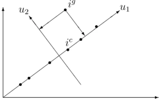
-6 ½½ ½½ ½½ ½½ ½½ ½½ ½ >u1 r r r r ic r r S S S S S S S S o u2 ri g ½ ½ ½ = S S S w
Figure 3: Supplementary points
For example, figure 3 shows how compromise points are contained in a subspace of dimension one, whereas the partial row profileig is in a two dimensional subspace.
8
Reconstructing distances between profiles
In § 2 the objective of Correspondence Analysis was defined as the search for subspaces that allow us to visualize the distances between profiles (row profiles or column profiles) as exactly as possible. The use of projections on all the dimensions obtained in the analysis allows us to reconstruct exactly theχ2 distances between two profiles (row or column). The
proposed Simultaneous Analysis also allows us to restore the χ2 distances between profiles
(row or column) of the same table.
To demostrate this we will bear in mind that“ a simple but particulary lemma is: a config-uration E is a Euclidean representation of B if BBT =EET” (Gifi 1991, chapter 8).
Distances between column profiles:
Let us denote as follows:
• Gis the matrix, of order (J×S), whose rowj contains the coordinates of the projection of column profile j on the S axes.
• V is the matrix, of order (I×S), whose columns are the eigenvectors, normalized for the usual Euclidean metric, of the matrix XXT.
To show that the distances between projections of the column profiles, included in G, of the same table reflect exactly theχ2 distances between column profiles we will show that G
is Euclidean representation of the matrix that we will denote by B and that the distances between rows of this matrixB are proportional to the χ2 distances between column profiles.
With the said notation we can express the projections of the column profiles (in equation (10) computed for axis s) as a function of the eigenvectors of the analysis and the matrices X and N defined in equations (8) and (12):
GGT = N−1/2XTV VTXN−1/2
Since matrix V is orthonormal, because it is an eigenvector matrix, the previous equation can be expressed as:
GGT = N−1/2XTXN−1/2
Denoting by B the matrix, of order (J×I), N−1/2XT whose generic term is:
√ αg q fi.g µ fijg fi.gf.jg −1 ¶
We can calculate the squared distance between rows j and j0 of this matrix when j and j0 belong to the same groupg:
d2 B(jg, j0 g) = X i∈I " √ αg q fi.g µ fijg fi.gf.jg −1 ¶ − √αg q fi.g à fijg0 fi.gf.jg0 −1 !#2 =
= X i∈I αg 1 fi.g à fijg f.jg − fijg0 f.jg0 !2 = = αg d2χ2(jg, j0g)
where the last distance is the χ2 distance between column profiles of the table g when it is
separately analyzed.
Distances between row profiles:
Let us denote as follows:
• F is the matrix, of order (IG×S), which contains the coordinates of the projections of the partial row profiles on the S axes. In this matrix the row that contains the projections of the partial row profileig on the S axes will be denoted byig.
• U is the matrix, of order (J ×S), whose columns are the normalized eigenvectors of the matrix XTX.
Then, we can express the projections of the set of partial row profiles (computed in equa-tion 14 for axis s) as a function of the eigenvectors us and the matrices Y and Q defined in
(13):
F FT = Q−1/2Y UUTYTQ−1/2
Since matrixU is orthonormal, because it is an eigenvector matrix, it is possible to express: F FT = Q−1/2Y YTQ−1/2
Denoting by C the matrix, of order (IG×J),Q−1/2Y whose generic term is:
( √ αg ³ fijg fi.gf g .j −1 ´ q f.jg if j ∈ Jg 0 if j 6∈ Jg (24) we can compute the squared distance between rows ig and i0g of this matrix, when both belong to the same groupg:
d2C(ig, i0g) = X j∈Jg · √ αg µ fijg fi.gf.jg −1 ¶ q f.jg − √αg µ fg i0j fig0.f.jg −1 ¶ q f.jg ¸2 = = X j∈Jg αg f.jg µ fijg fi.gf.jg − fig0j fig0.f.jg ¶2 = = X j∈Jg αg 1 f.jg µ fijg fi.g − fig0j fig0. ¶2
The last distance is the χ2 distance between two row profiles of tableg, once weighted with
αg, when it is separately analyzed. As a result its is shown that Simultaneous Analysis
restores the original distances between partial row profiles using their projections.
9
Reconstructing original data
As mentioned in§5, once the matrixX is defined, the eigenvectors (of both row analysis and column analysis) are calculated by performing a principal component analysis. Therefore, the reconstruction of the matrix X as a function of eigenvectors has the same expression as in principal component analysis:
X = X
s
λ1s/2vsuTs
To reconstruct the matrix as a function of coordinates, we transform the above equation and recall that the computation of the projections obtained in (9) and (10) does not match the expression using matrices of principal component analysis or correspondence analysis:
X = X s λ1s/2 R1/2 R−1/2vs uTsN−1/2 N1/2 = = R1/2 Ã X s λ−s1/2Fs(Ic)Gs(J)T ! N1/2
One element of the above mentioned matrix is: xij = Ã X g∈G q fi.g ! Ã X s λ−s1/2Fs(ic)Gs(j) !q f.jg
This is the matrix defined in equation (8) and therefore: fijg fi.gf.jg −1 = 1 √ αg X g∈G q fi.g p fi.g X s λ−s1/2Fs(ic)Gs(j) Spliting fijg up we obtain: fijg = fi.gf.jg 1 + 1 √ αg X g∈G q fi.g p fi.g X s λ−s1/2Fs(ic) Gs(j)
10
Application to the Survey on Stolen Articles
To show the importance of maintaining the χ2 distances computed in studying each
contin-gency table separately when they are to be analysed jointly, we next present an application with the information of the example “shoplifting 1977/1978” by Isra¨els (1987).
In this example there are considered to be two contingency tables, one for men and another for women derived from the ternary table that classifies a population of suspects of theft in big stores in Holland, according to sex, age (classified in 9 modalities) and the type of article stolen (CLOT: Clothing, CLAC: Clothing accesories, TOBA: Provisions, tobacco, WRIT: Writing materials, BOOK: books, RECO: records, HOUS: household goods, SWEE: sweets, TOYS: toys, JEWE: jewelry, PERF: perfume, HOBB: hobbies, tools, and OTHE: other). Since the interest of the present application is not focused on the study of the information and on the relations between the variables, we will only mention those aspects that help us to show the importance of the treatment of the distances in maintaining the internal relationships within each table.
To that end, we present the planes of the Correspondence Analyses of the separated tables for men and women, the Intra Analysis of both tables and the proposed Simultaneous Analysis (figure 4). The plane of the juxtaposition, and its interpretation -very different from those discussed below-, and of the separated analyses can be found in the paper cited (Isra¨els 1987). A detailed account of the results of the analyses cited can also be found in Goitisolo (2002).
As a short interpretation it is possible to say that in the planes of the separate analyses it is observed that the categories of age are projected following a curvilinear line. It is observed that in the factorial plane of Simultaneous Analysis the internal structure of each table is maintained quite faithfully, which is not the case in the plane of the Intra Analysis.
The first factor shows how the youngest people, up to 14 years, are attracted, fundamentally, by the theft of toys -TOYS-, sweets -SWEE- and writing materials -WRIT- unlike the people of middle age, who are more attracted, when it comes to stealing, by the clothes -CLOT-. In the example, the differences are shown in the second factor. In the case of the men’s table, it is basically shown that interest in the theft of jewels -JEWE- and of music -RECO- is low among children under 12 and people over 65 and high in teenagers from 15 to 17, whereas in the women’s table, the second factor reveals the strong attraction that the theft of tobacco -TOBA- has among women over 65, who are not however attracted by the theft of clothing -CLOT- and jewelry -JEWE-, which is more common in women aged 18 to 30 and 15 to 17, respectively.
In Intra Analysis, this second factor shows the attraction of women from 21 to 39, for the theft of clothing -CLOT-. The second factor of Simultaneous Analysis indicates that women over 65 are more inclined to steal tobacco -TOBA- than jewels -JEWE- or music -RECO-, which are more commonly stolen by women from 12 to 17. This is observed in the separate analysis of the table relating to women.
In reference to the weighting that balances the influence of the tables in Simultaneous Anal-ysis we can indicate that, provided that the eigenvalues associated with the first factors are similar in both tables, the differences observed between Intra Analysis and the proposed Si-multaneous Analysis are due, in this example, almost exclusively to the different definitions of distance used between profiles and not to the weights introduced.
11
Conclusions
This paper shows how it is possible to carry out a factor analysis of a set of contingency tables in which within relations of each table are maintained. These relations in a contin-gency table are usually analyzed using the χ2 distance between profiles of the table. The
generally accepted use of this distance is backed up by its relationship with the Pearson χ2
statistic to study the independence between two qualitative variables and by its principle of distributional equivalence. Maintaining these distances in the study of more than one contingency table is therefore essential in order not to alter the relationships studied in each table.
References
Benz´ecri, J.P. & collaborateurs (1973), L’ Analyse Des Donn´ees. 2: L’ Analyse Des Corre-spondances, Dunod.
Escofier, B. & Pag`es, J. (1998),Analyses Factorielles Simples et Multiples. Objetifs, m´ethodes et interpr´etation, 3 edn, DUNOD.
Gifi, A. (1991),Nonlinear Multivariate Analysis, Wiley.
Goitisolo, B. (2002), El An´alisis Simult´aneo. Propuesta y Aplicaci´on de un Nuevo M´etodo de An´alisis Factorial de Tablas de Contingencia, Tesis doctoral, Universidad del Pa´ıs Vasco.
Isra¨els, A. (1987),Eigenvalue Techniques for Qualitative Data, DSWO Press.
Lebart, L., Morineau, A. & Piron, M. (1995), Statistique Exploratoire Multidimensionnelle, Dunod.
L’Hermier des Plantes, H. (1976), STATIS: Structuration de Tableaux `A Trois Indices de la Statistique, Th`ese (3c), USTL, Montpellier.
M´eot, A. & Leclerc, B. (1997), ‘Voisinages a priori et analyses factorielles: Illustration dans le cas de proximit´es g´eographiques’, Revue de Statistique Appliqu´eeXLV, 25–44. Torre, F. & Chessel, D. (1995), ‘Co-structure de deux tableaux totalement appari´es’,Revue
Z´arraga, A. & Goitisolo, B. (2002), ‘M´ethode factorielle pour l’ analyse simultan´ee de tableaux de contingence’, Revue de Statistique Appliqu´eeL(2), 47–70.
Z´arraga, A. & Goitisolo, B. (2003), ‘´Etude de la structure inter-tableaux `a travers l’ Analyse Simultan´ee’, Revue de Statistique Appliqu´eeLI(3), 39–60.
Z´arraga, A. & Goitisolo, B. (2006), Simultaneous analysis: A joint study of several con-tingency tables with different margins, in M. Greenacre & J. Blasius, eds, ‘Multiple Correspondence Analysis and Related Methods’, Chapman & Hall/CRC, Boca Raton, Fl, pp. 327–350.