PREPROCESSING AND ANALYSIS
OF SINGLE-CELL
RNA-SEQUENCING DATA
Master’s Thesis
Degree Programme in Biotechnology Faculty of Medicine and Life Sciences University of Tampere, Finland
Meeri Pekkarinen May 2018
i MASTER’S THESIS
Place: University of Tampere, Faculty of Medicine and Life Sciences
Author: Meeri Pekkarinen
Title: Preprocessing and analysis of single-cell RNA-sequencing data
Pages: 55 pages + an appendix
Supervisors: Dr.Tech Juha Kesseli, M.Sc Antti Ylipää Reviewers: Professor Matti Nykter, Dr.Tech Juha Kesseli
Date: May 2018
ABSTRACT
In recent years, single-cell measurement technologies have greatly advanced and offer a new approach to study biological problems. While the traditional RNA sequencing results in computational average transcriptome that represents the whole biopsy, scRNA-sequencing records the transcriptional differences between the cell types. However, the method is also more sensitive to various biological and technical noise, and the field still calls for further research and establishment. Especially data normalization and quality control require novel methods, since many of the tools originally developed for bulk RNA-seq data are based on assumptions that are not valid for scRNA-seq data.
The goal of this thesis was to gain insight in RNA-seq analysis and especially find the optimal ways to preprocess the data and asses its quality. The relevant tools were chosen and further tested in the computational part of the thesis. The final and the most important deliverable was an analysis pipeline constructed by combining the best approaches and necessary quality metrics.
A three-step pipeline utilizing various command line tools and Bioconductor R-packages was implemented. This pipeline performs preprocessing, transcript quantification, filtering, normalization and simple downstream steps. Most importantly, it produces both visual and statistical information for estimating various general features and quality properties of the data. The pipeline was successfully used to process two public scRNA-seq datasets.
The work was done for Genevia Technologies Oy in Tampere between October 2017 and May 2018. An ultimate goal was to develop a generalized pipeline that would be useful to the company. However, diverse analytical and technical issues make this task very challenging, and a couple of pitfalls still remain unsolved. One major reason is that no best practices are yet established. Regardless, the information provided by the pipeline should be helpful for picking suitable tools and thresholds for more sophisticated methods. Future development in the field will most certainly discover biological information that cannot be discerned by current tools.
ii PRO GRADU -TUTKIELMA
Paikka: Tampereen yliopisto, Lääketieteen ja biotieteiden tiedekunta
Tekijä: Meeri Pekkarinen
Otsikko: Preprocessing and analysis of single-cell RNA-sequencing data Sivumäärä: 55 sivua, 1 liitesivu
Ohjaajat: TkT Juha Kesseli, DI Antti Ylipää Tarkastajat: Prof. Matti Nykter, TkT Juha Kesseli
Päiväys: Toukokuu 2018
TIIVISTELMÄ
Solun molekulaaristen ominaispiirteiden määrittämiseen on hiljattain kehitetty RNA-sekvensointimenetelmä, jolla voidaan tutkia yksittäisten solujen mRNA-tuotantoa suurella tarkkuudella. Menetelmästä käytetään nimeä scRNA-seq (single-cell RNA-sequencing). Aikaisemmin RNA-sekvensoinnissa (bulk RNA-seq) on voitu mitata isojen solupopulaatioiden keskimääräistä käyttäytymistä, mutta ei ole pystytty erittelemään solutyyppien tarkkoja piirteitä tai seuraamaan kehittyvissä solupopulaatioissa tapahtuvaa monimutkaista molekulaarista evoluutiota. Uusi sekvensointimenetelmä avaa kiinnostavia mahdollisuuksia biologisten ilmiöiden syvällisempään ymmärtämiseen ja tiedon soveltamiseen esimerkiksi taistelussa syöpää vastaan. Toisaalta tarkkuus tekee menetelmästä herkemmän erilaisille teknisille ja biologisille vääristymille, mikä asettaa haasteita erityisesti datan esikäsittelylle, laatuanalyysille ja normalisoinnille. Päivitettyjä laskennallisia ja analyyttisiä metodeja tarvitaan, sillä monet aikanaan RNA-sekvensointidatalle kehitetyt työkalut tekevät datasta tietynlaisia oletuksia, jotka eivät välttämättä päde scRNA-datalle. Tämän Pro gradu -tutkielman tarkoitus oli perehtyä scRNA-sekvensointiin ja työkaluihin, jotka on räätälöity ottamaan huomioon datan aiheuttamat haasteet. Lisäksi työn tärkein tavoite oli suunnitella ja toteuttaa analyysivuo, joka suorittaa datalle automatisoidun esikäsittelyn sisältäen mm. laatuanalyysin, suodatuksen ja normalisoinnin. Tutkielma toteutettiin yhteistyössä GeneviaTechnologies Oy:n kanssa Tampereella, ja sitä työstettiin lokakuusta 2017 toukokuuhun 2018.
Työn tuloksena syntyi kolmeosainen analyysivuo, joka yhdistelee useita uusimpia työkaluja shell- ja R-pohjaisten skriptien avulla. Analyysivuon keskeisimmät vaiheet ovat sekvensointitiedostojen laatuanalyysi ja suodatus, geeniekspression kvantifiointi referenssitranskriptomia vasten sekä tuloksena syntyvän matriisin suodatus, visualisointi ja normalisaatio. Lisäksi sovellettiin muutamaa korkeamman tason työkalua, joilla voitiin tehdä datasta yksinkertaisia biologisia johtopäätöksiä ja arvioida osien toimintaa. Analyysivuon avulla prosessoitiin kahta julkista scRNA-datasettiä, ja sen räätälöitävyyttä pyrittiin parantamaan konfiguraatiotiedoston avulla.
Päämäärä oli tuottaa analyysivuo, jota voidaan tulevaisuudessa soveltaa myös yrityksen tarpeisiin. Mahdollisia analyysiin vaikuttavia muuttujia, sekä datalähtöisiä että teknisiä, on kuitenkin varsin paljon, eikä kaikkiin ongelmakohtiin ole vielä kirjallisuudessakaan kehitetty yleiskäyttöistä ratkaisua. Näinollen tämäkään analyysivuo ei sellaista tarjoa, ja tuloksia on osattava aina tarkastella kriittisesti ja mahdollisesti täydennettävä analyysiä räätälöidyillä menetelmillä. Ala kuitenkin kehittyy nopeasti, ja tulevaisuudessa on odotettavissa uusia, tarkempia menetelmiä ja mielenkiintoisia löytöjä.
iii
Acknowledgements
This thesis was an adventure that I could not have been able to complete without the help of several people. First, I am very grateful to my supervisors, Juha Kesseli and Antti Ylipää for feedback, trust and good discussion. My thanks also for Professor Matti Nykter for arranging the computational capacity from CSC and reviewing the written thesis. Moreover, Matti Annala kindly helped me to get started with the computational environment. I also want to thank the whole Genevia team for the support, trust and wonderful working environment! It has been such a pleasure to get to know you all, and I think there was not a single day without at least one good laugh and excellent coffee, even though sometimes certain challenges felt bigger than I could handle.
I probably would not be alive without my beloved husband Esko who has supported me in such many ways during my thesis and studies. In addition to his endless patience and love, he also helped me with the grammar and provided valuable insight as a software developer. Thanks also to my dear friends and siblings for patience, encouragement and providing some down time in situations where I really needed a break.
Finally, I would like to thank my wonderful parents who have trusted in me for all these years and always encouraged my interest towards science and nature.
Meeri Pekkarinen May 2018
iv
Abbreviations
HISAT Hierarchical indexing for spliced alignment of transcripts
IVT In vitro transcription
EM Expectation-Maximization algorithm
LMM Linear mixture model
LVM Latent variable model
MAD Median absolute deviation
MAST Model-based analysis of single cell transcriptomics
PCA Principal component analysis
PLS Partial Least Squares
SC3 Single-Cell Consensus Clustering
SCA SingleCellAssay (a data object in R)
SCE SingleCellExperiment (a data object in R) SLURM Simple Linux Utility for Resource Management STAR Spliced Transcripts Alignment to a Reference tSNE T-Distributed Stochastic Neighbor Embedding
v
Table of Contents
1 Introduction ... 1
2 Literature review ... 3
2.1 Experimental design and quantitative standards ... 3
2.2 Initial quality control and pre-processing of raw reads ... 4
2.3 Gene expression quantification ... 7
2.3.1 Alignment-based approaches ... 7
2.3.2 Alignment-free approaches ... 8
2.4 Quality control and filtering of the expression matrix ... 10
2.4.1 Celloline and cellity ... 12
2.4.2 Scater ... 12
2.5 Normalization ... 14
2.5.1 Principles of global-scaling normalization ... 15
2.5.2 Deconvolution-based scaling normalization and scran-package ... 17
2.5.3 Quantile-regression based normalization and SCnorm ... 18
2.6 Confounding factors ... 19
2.7 Obtaining biological insights... 20
2.7.1 SC3: Cell type identification by consensus clustering ... 21
2.7.2 Determining cell lineage and differentiation ... 22
3 Objectives... 24
4 Materials and methods ... 25
4.1 Data ... 25
4.2 Environment and the relevant tools ... 25
4.3 Filtering, normalization and confounders ... 27
4.4 Downstream analyses ... 27
4.5 Comparing pipeline results into the literature ... 27
5 Results ... 29
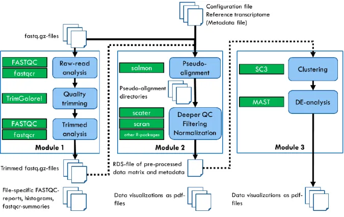
5.1 The pipeline ... 29
5.1.1 Module 1: Initial quality processing ... 29
5.1.2 Module 2: Quantification, further QC-processing and normalization ... 30
5.1.3 Module 3: Clustering and DE-analysis ... 31
5.2 Initial quality checks and trimming with Module 1 ... 31
5.3 Pipeline visualizations for estimating dataset quality before filtering ... 34
5.4 Filtering ... 37
5.5 Checking the features with the highest expression over cells ... 38
vi
5.7 Confounders ... 40
5.8 Clustering with SC3 ... 41
5.9 Applying tSNE for preprocessed Darmanis ... 45
6 Discussion ... 47
7 Conclusions ... 52
8 References ... 53
1
1
Introduction
Traditional high-throughput RNA sequencing i.e. RNA-seq derives genome-wide mRNA expression data from samples consisting of large cell populations. The product is one averaged expression profile to represent the whole biopsy which may easily oversimplify the biological functionality (Bacher & Kendziorski 2016). Thus, the approach is insufficient for studying complex tissues and biological conditions, where the cells have diverse expression profiles (Stegle et al. 2015). Single-cell RNA sequencing i.e. scRNA-seq aims to solve this problem by recording the expression profiles of the samples that each consist of the amplified mRNA (cDNA) of a distinct cell (Poirion et al. 2016; Bacher & Kendziorski 2016; Stegle et al. 2015). An overview of a typical experiment is presented in Figure 1.
Figure 1: An overview of a scRNA-seq workflow (https://hemberg-lab.github.io/scRNA.seq.course 12/16/2017). The cells in a biopsy are gently dissociated and collected in separate pools before extracting the mRNA. After converting RNA into cDNA, the material from each cell is amplified by polymerase chain reaction (PCR) or alternatively, by In vitro transcription (IVT) combined with reverse transcription (RT). Sequencing is followed by complex data processing and downstream analysis to finally obtain biological insights, e.g. identifying the cell-subpopulations.
2
The progress of scRNA-seq technologies enables diverse new applications. These include for example 1) Recording the diverse expression patterns in embryonic development, 2) Identification of novel cell types and 3) Getting broader insight of transcription control (Arzalluz-Luque et al. 2017; Ofengeim et al. 2017). It also gives new insight for understanding the development and progression of medical conditions such as cancer (Yuan et al. 2017). When the roles of tumor microenvironments can be examined more precisely and the mechanisms behind disease progression and drug resistance are resolved, novel efficient treatments can be developed.
Even though being a powerful approach for biological discovery, the cost is that processing and interpretation of scRNA-seq data is far from trivial (Bacher & Kendziorski 2016; Poirion et al. 2016; Stegle et al. 2015). The analysis flow resembles the traditional RNA-seq data analysis (expression quantification, quality control and normalization followed by downstream analysis for biological insights), but the distinct features of scRNA-seq data require novel approaches. The key challenge in analysis is that scRNA-seq data is heterogeneous i.e. there is remarkable level of both biological and technical cell-to-cell variation (Yuan et al. 2017). This makes especially the QC and normalization of the data tremendously challenging. Moreover, the size of the datasets produced by experiments can be enormous: even thousands to tens of thousands samples in a single experiment (Ilicic et al. 2016). The sequencing depth and thus the sizes of sequencing libraries vary from tens of thousands to millions of reads per cell (Andrews & Hemberg 2018). Finally, since the field is still quite young, the amount of data and established standards is still marginal. As stated by Andrew&Hemberg, scRNA-seq is not a single method but a collection of protocols designed for various applications that have differing strengths and limitations.
The major focus in this thesis is in the early steps of the analysis flow, especially quality control (QC) and normalization. The objectives are 1) Looking for an optimal way to preprocess scRNA-seq data and asses its quality, 2) Testing and comparing the relevant tools with different publically available datasets and 3) Constructing the analysis pipeline by combining the best approaches and necessary quality metrics. In literature review, some current approaches and relevant insights for scRNA-seq data processing are discussed.
3
2
Literature review
2.1
Experimental design and quantitative standards
Even though being outside of the major context of this thesis, it should be noted that experimental design may affect the downstream analysis and data interpretation (Bacher & Kendziorski 2016). For example, the protocol-specific rate of how efficiently the cells are captured as distinct samples and not cell doublets or their multiples may be critical when identifying novel cell types (Andrews & Hemberg 2018). For more detailed discussion of different protocols, see e. g. (Ziegenhain et al. 2017) and (Svensson et al. 2017). Due to the experimental properties, some of the analysis tools are platform-specific. Moreover, there are tools that may be based on certain quantitative standards (Bacher & Kendziorski 2016). The establishment of quantitative standards is still in progress, and there are also differing opinions on their usage. For example, Stegle et al. strongly recommend the usage of the two standards i.e. extrinsic spike-in RNA molecules and unique molecular identifiers (Stegle et al. 2015). On the other hand, they as well as Bacher&Kendziorski mention that even though both have theoretical advantages for normalization and expression estimation, there are some practical challenges and restrictions that have prevented their routine usage (Bacher & Kendziorski 2016).
Spike-in RNA refersto synthetic or exogenous RNA that is added into each sequencing library at known concentration, thus working as an internal control (Stegle et al. 2015). When used, their sequences should be added into the reference genome or transcriptome prior to mapping (Stegle et al. 2015). Spike-ins help estimate relative differences in RNA content by attributing the differences between the observed and expected expressions of spike-ins to technical errors, which should improve normalization (Bacher & Kendziorski 2016). Normalization with spike-ins is generally done by calculating a cell-specific spike factor that adjusts for the difference, and then applying this factor to endogenous genes (Bacher & Kendziorski 2016).
Unique molecular identifiers (UMIs) are short (6-10 nucleotides) and random sequences that are attached to individual molecules of interest before PCR-amplification (Stegle et al. 2015). They make each molecule unique and allow the following of absolute molecular count and further accounting of amplification biases (Bacher & Kendziorski 2016). When UMIs are used, the barcode attached to each read should be removed before mapping (Stegle et al. 2015). In normalization phase, assuming that each cDNA-molecule of the library is observed at least once, the number of UMIs linked to each gene is the direct measure of the number of cDNA
4
molecules associated with that gene (Stegle et al. 2015). This still does not fully exclude the technical sources of expression variability.
2.2
Initial quality control and pre-processing of raw reads
FASTQ-files may contain varying proportions of low-quality reads/sub-reads and synthetic sequences (e.g. UMIs discussed in Chapter 2.1) which are commonly removed before alignment (Bacher & Kendziorski 2016). However, read trimming can be done with several options and stringencies, and currently there seems to be no consensus of the best practice. It was also recently shown that even though read trimming generally improves the mapping rates, aggressive quality-based trimming may distort the expression estimation (Williams et al. 2016). Some quality filtering of the samples may be done in this early phase of analysis flow, even though the full picture of the quality is obtained only after mapping. The decision of which cells (or reads) to include is not always trivial, even though many preprocessing tools suggest some thresholds for bulk RNA-seq data (Bacher & Kendziorski 2016). The amount of tools specifically developed for scRNA-seq quality control is still small, even though some ready-made pipelines exists (Poirion et al. 2016, Ilicic et al 2016) Suggested individual tools are FASTQC (http://www.bioinformatics.babraham.ac.uk/projects/fastqc/, 11/10/2017) or Kraken (Davis et al.2013), which are used both before and after alignment (Bacher & Kendziorski 2016; Stegle et al. 2015). In general, for example empty sequencing libraries, samples that contain remarkably low amounts of reads as well as the cells that contain suspiciously high amounts of low-quality reads can be discarded prior to expression estimation.
FASTQC is an example of generic QC tool which provides diverse within-sample quality information and graphics (see Table 1). It also helps to check whether the low quality samples follow a certain pattern. For example, according to Bacher and Kendziorski, systematic low scores in the beginning of the read may indicate some problem with the run and should not be trimmed, while low scores in the read tails indicate a general degradation, in case which trimming may be useful (Bacher & Kendziorski 2016).
5
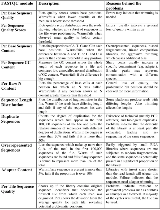
Table 1: Quick review of the modules of FASTQC-tool
(https://www.bioinformatics.babraham.ac.uk/projects/fastqc/, 4/11/2018). Quality properties are examined as several modules to check whether the sample passes or causes a warning or a failure according to defined criteria.
FASTQC module Description Reasons behind the
problems Per Base Sequence
Quality
Plots quality scores across base positions. Warns/fails when lower quartile or the median is below some threshold
Errors may indicate that trimming is needed
Per Sequence Quality Scores
Plots quality score distribution over the reads, showing whether any subset of sequences in the file were problematic. Warns/fails when observed mean quality is below certain threshold
Errors usually indicate a general loss of quality within a run
Per Base Sequence Content
Plots the proportions of A, T, G and C in each base positions. Warns/fails when the difference between A and T, or G and C is greater than certain threshold in any position
Overrepresented sequences, biased fragmentation, Biased composition libraries, too aggressive trimming which causes additional bias
Per Sequence GC Content
Measures the GC content across the whole length of each sequence in a file and compares it to a modelled normal distribution of GC content. Warns/fails if the difference is big enough
Sharp peaks usually indicate a specific contaminant (e.g. adapter). Broader peaks may represent contamination with a different species.
Per Base N Content
Plots the percentage of base calls at each position for which an N was called. Warns/Fails if any position shows an N content greater than certain threshold
General loss of quality, the problematic bin position should be checked for more information.
Sequence Length Distribution
Plots the distribution of fragment sizes in the file. Warns if the reads have differing length and fails if any of the sequences has zero length
Some platforms produce reads with differing lengths. Also trimming affects the lengths
Duplicate Sequences
Counts the degree of duplication for the sequences which first appear in the first 100,000 sequences of the file and plots the relative number of sequences with different degrees of duplication. Warns if the degree is more than 20% and fails if it is more than 50%
Existence of technical (mainly PCR artefacts) and biological duplicates. Problems indicate that the diversity of the library is at least partially exhausted, leading into re-sequencing of the same sequences.
Overrepresented Sequences
Lists the sequence which make up more than 0.1% of the total in the first 100,000 sequences of the file. Warns if such sequences are found and fails if any sequence is found to represent more than 1% of the total.
Easily triggered by small RNA libraries where sequences are not subjected to random fragmentation, and the same sequence is potentially present in a significant proportion of the library
Adapter Content Warns if any sequence is present in more than 5%, fails if the proportion is over 10%
Libraries with insert sizes shorter than the read length will trigger this module. Failure indicates that the sequences need adapter trimming.
Per Tile Sequence Quality
Shows up if the library contains original sequence identifiers that document the flowcell tile from which each read was originated. Plot shows the deviation from the average quality for each tile, revealing potential problematic positions.
Problems indicate transient or permanent problems such as bubbles or smudges in a flowcell. If majority of the cycles was useful, the file can be used.
6
A dataset-wide summarization tool for analyzing FASTQC-results is useful, since the potentially large amount of samples make manual checking of each sample impossible or at least time-consuming. An example of this kind of tool is an R-package fastqcr (http://www.sthda.com/english/rpkgs/fastqcr/index.html 11/10/2017).
Adapter contamination refers to the occurrence of experimental add-on sequences that do not provide any biological information (https://www.ncbi.nlm.nih.gov/tools/vecscreen/contam/, 12/12/2017). Adapter sequences can be obtained e.g. by FASTQC which detects the overrepresented sequences, or from the sequencing protocol documentations. There are several tools designed for removing this kind of sequences from the raw reads, see e.g. http://bioscholar.com/genomics/tools-remove-adapter-sequences-next-generation-sequencing-data/ (11/17/2017). One of these tools is cutadapt, which can be used to trim adapter sequences, primers, poly-A tails and other types of unwanted sequences (Martin 2011). Cutadapt algorithm calculates optimal alignments between each read and all given adapters/unwanted sequences, and trims the sequence if the error rate is below an allowed maximum. The error rate is calculated as the number of alignment errors divided by the length of the matching segment between the read and the adapter.
A wrapper script TrimGalore! by Babraham Institute combines FASTQC analysis and cutadapt and is an example of the pipeline that aims to automate the initial quality control procedure (http://www.bioinformatics.babraham.ac.uk/projects/trim_galore 11/17/2017). It combines both quality and adapter trimming and can be used for any high throughput dataset, both paired and single-end reads. By default, it auto-detects some common adapters (Illumina universal, Nextera transposase and Illumina small RNA adapter sequence), but specific adapter sequences to be trimmed can also be provided. Quality trimming of the read ends based on FASTQC Phred scores can be adjusted. After trimming, the reads shorter than a given threshold can be removed. Unknown bases (Ns) can be removed from either side of the reads.
Krishnaswami et al. mention that deep sequencing tends to produce many duplicate sequences of abundant transcripts (Krishnaswami et al. 2016). These duplicates reduce the ability to detect low-copy transcripts, but cannot be removed, since that would disturb accurate expression quantification. They recommend the evaluation of the sequence duplication proportion so that it can later be used to examine potential impact on low-copy transcripts. A tool that can be used for this is FASTQ/A Collapser of FASTX toolkit (http://hannonlab.cshl.edu/fastx_toolkit/, 11/17/2017).
7
2.3
Gene expression quantification
The ultimate goal of gene expression quantification is to collect the expression measures of all the genes (or transcripts) in all the samples into one expression matrix. In the traditional two-step procedure, the preprocessed reads are first aligned against the reference sequence and the mapped reads are then summarized with a separate tool to generate the read counts (Engström et al. 2013; Jin et al. 2017; Stegle et al. 2015). Notably, also some alignment-free approaches have been recently developed, and they are shown to be remarkably faster than any of the usual aligners, and still have similar or even better accuracy (Patro et al. 2017; Zielezinski et al. 2017). These tools encompass the tasks analogous to alignment and quantification into a single tool, making the early steps of analysis easier and faster. However, sometimes the exact mapping information is needed in downstream analysis, e.g. when looking for novel transcripts, and in such cases, alignment-free tools cannot be used.
Quantification approach is one of the several factors that may influence on the subsequent analysis and interpretation of the data, since alignment tools differ in performance and accuracy. Overall consensus of an optimal method still does not exist, and there are no approaches designed specifically for scRNA-seq experiments (Jin et al. 2017; Poirion et al. 2016). However, the fast increase in data sizes already challenges both storage and processing capacities of computers (Zielezinski et al. 2017). Since scRNA-experiments may produce remarkably large datasets, the memory-effectiveness is inevitably a crucial feature when trying to resolve the computational bottleneck in gene expression quantification.
2.3.1 Alignment-based approaches
An alignment-based method for transcriptomic data should solve two computationally expensive problems (Dobin et al. 2013). The first is, like in any alignment task, how to accurately align reads containing mismatches and indels i.e. insertions or deletions. The second and transcriptomics-specific problem is, how to deal with the reads containing sequences from non-contiguous genomic regions i.e. from various exon-exon boundaries resulting from RNA splicing. Moreover, as a result of genomic evolution there may be multiple identical or related genomic regions that are all transcribed: how to align the reads that map in multiple sites in the genome?
There is a broad amount of alignment tools to choose from: for example Engström et al. evaluated as many as 26 mapping protocols based on 11 programs and pipelines (Engström et al. 2013). A common feature for all alignment-based programs is that they look for
8
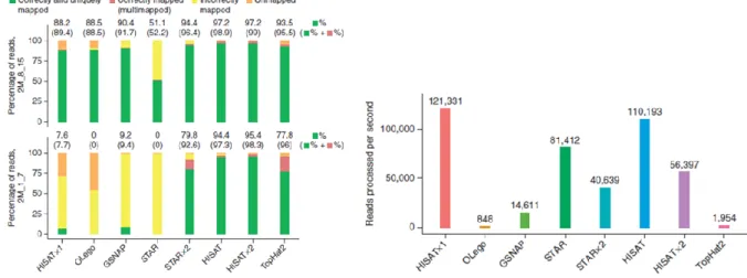
correspondence of individual bases that are in the same order in the sequences they are comparing (Zielezinski et al. 2017). They assume that every character of the sequence can be categorized at least into match or mismatch, and most approaches also recognize indels. Based on the comparative analysis by Engström and colleagues, STAR (Spliced Transcripts Alignment to a Reference, see (Dobin et al. 2013)) seemed to outperform most of the other approaches based on different performance benchmarks. On the other hand, Kim et al. later showed that HISAT (Hierarchical Indexing for Spliced Alignment of Transcripts) was the most efficient when using two simulated datasets, as seen in Figure 2 (Kim et al. 2015). However, it should be noted that sequence alignment depends on multiple a priori assumptions about the evolution of the sequences, and these with other parameters are user-defined and therefore more or less artificial (Zielezinski et al. 2017). Modifying parameters, as well as using another aligner program with potentially differing scoring system may lead in very different results, and this makes the choice of best or most accurate approach quite challenging.
After the alignment, the gene counts are generated with the tool of choice, for example HTseq or cufflinks (Bacher & Kendziorski 2016; Ilicic et al. 2016). Useful functionality may also be provided by the aligner, for example STAR has the option “quantMode” which generates the read counts. However, the layout of these files may differ from the commonly used alternatives, and may require some additional formatting.
2.3.2 Alignment-free approaches
Recently it has been found out that exact alignments of the reads against the reference genome are not crucial for the reliable estimation of transcript levels (Zielezinski et al. 2017). Instead,
Figure 2: Comparison of some most common RNA-seq aligners (Kim et al. 2015). Two simulated datasets were used to measure mapping quality and the alignment speed, respectively.
9
the reads can be compared against the reference transcriptome and find the transcripts from where the queries have most probably originated from (Jin et al. 2017; Srivastava et al. 2016). Most of these kind of alignment-free algorithms are either word-frequency based methods that calculate the frequencies of subsequences (k-mers) of a defined length, or information-theory based methods that evaluate the informationalcontent between full-length sequences (Zielezinski et al. 2017).
Programs kallisto (Bray et al. 2016; https://pachterlab.github.io/kallisto, 11/9/2017) and Salmon (Patro et al. 2017; http://salmon.readthedocs.io/en/latest/salmon.html 11/9/2017) are examples of recently developed alignment-free approaches for expression quantification. They require much less computational capacity than traditional aligners, and are thus particularly useful with large datasets. In addition to expression quantification, alignment-free methods have also been developed for other tasks such as variant calling (Zielezinski et al. 2017). Pseudoalignment algorithm kallisto builds a deBruijn graph from the k-mers of the reference and, for each read, uses that graph to define an equivalence class i.e. a multi-set of transcripts associated with the read (Bray et al. 2016). From these pseudoalignments, the transcript abundances are then quantified with a likelihood function which is iteratively optimized with the Expectation-Maximization (EM) algorithm. Moreover, the uncertainty of abundance estimates can be quantified by bootstrapping, and a model for correcting sequence-specific bias can be used. The program requires only the k-mer length and the mean of the fragment length distribution for expression quantification. K-mer length applied for the reference must be set large enough to avoid mappings of random sequences but short enough for error-robust mapping. Recently, the developers have updated kallisto with a mode specifically developed for scRNA-seq experiments (https://pachterlab.github.io/kallisto/singlecell.html, 4/8/2018). Quasi-mapping algorithm Salmon is also based on k-mers, and is built on statistical (Bayesian) interference procedure which enables the building of a probabilistic model of the experiment to quantify the reads (Patro et al. 2017). The position and orientation of all mapped fragments are tracked and combined with the calculated abundances, resulting in per-fragment conditional probabilities. According to Patro et al, Salmon is the first available method which has sample-specific models for positional, sequence-sample-specific and GC-dependent biases. Similar to kallisto, the uncertainty of abundance estimates can be assessed. In addition to the quasi-mapping mode, salmon also has the alignment-based mode than can be used to quantify the expression
10
based on the mapping results (BAM-files) of some other aligner. However, also with this mode the reads has to be originally aligned against a transcriptome, not a genome.
The principles of kallisto and Salmon are similar, even though underlying algorithms are different. The final output for both contains the counts presented as transcripts per million (TPM), meaning that the feature counts are first divided by the length of each feature in kilobases, and the results are then divided by a sample-specific “per-million” scaling factor. Moreover, a set of additional useful information e.g. bootstrapping and bias correction information and mapping metadata is provided.
2.4
Quality control and filtering of the expression matrix
The final product of gene expression quantification is the expression matrix containing n features and p samples together with various metadata of the mapping. Based on this data, the low-quality samples should be removed from subsequent analysis. Low-quality in scRNA-seq samples refers to 1) stressed/broken cells with degraded RNA or aberrant expression patterns, 2) samples that contain material from more than one cell (sometimes referred as doublets) and 3) empty samples resulted from either failed cell isolation or failed/premature cell lysis (Bacher & Kendziorski 2016; Ilicic et al. 2016).
Ready-made pipelines for QC exists, but they are not necessary well generalized: they may be platform-specific or compatible only with certain tools (Poirion et al. 2016). As an alternative, there are couple of toolkits for tailored analysis, providing approaches not only for QC but also further steps in analysis flow. Examples are Seurat (Satija et al. 2015) and scater (McCarthy et al. 2017). Each approach typically has a different representation for the data. For example, Seurat stores the data in its own Seurat-class, while scater uses SingleCellExperiment-class by Lun & Risso (http://bioconductor.org/packages/release/bioc/html/SingleCellExperiment.html, 5/3/2018).
Examining the technical features, like how well RNA was captured and amplified from each cell, is extremely important in scRNA-seq experiments (Bacher & Kendziorski 2016; Stegle et al 2015). One this kind of quality metric is the fraction of mapped reads back to genome: low rates may indicate RNA-degradation, contamination or inefficient cell lysis. If spike-ins were used, the ratio of the number of reads mapped to endogenous RNA to the number of reads mapped to extrinsic spike-ins should be calculated. If this ratio is small (i.e. there is a high proportion of reads mapped to spike-ins), the capturing of the decent proportion of mRNA-content of the cell has potentially failed.
11
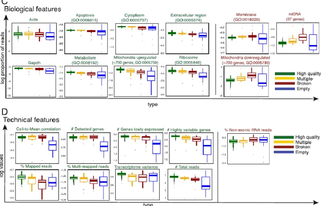
The factors that should be taken into account in scRNA-seq QC arevery comprehensively discussed by Ilicic et al 2016. They investigated both biological and technical features that differ in normal and quality cells (see Figure 3). For example, they showed that the low-quality cells have higher average gene expression in specific functional GO-categories and also noisier expression profiles in these categories. Genes relating to GO-terms Cytoplasm, Metabolism and Membrane were generally downregulated in broken cells, while Mitochondrially encoded genes and Mitochondrially localized proteins seemed upregulated. The loss of cytoplasmic content of damaged cells before the experimental cell lysis and resulting increase in the relative proportion of mitochondrial content is suggested as explanation for mitochondrial upregulation.
Aevermann et al. have also investigated approaches for quality classification of single-cell and single-nuclei RNA-seq samples, and found differing results compared to Ilicic et al. (Aevermann et al. 2016). According to their random forest -based analysis, they suggest that metrics such as the ratio of trimmed reads over raw reads and percent of duplicated reads could be useful as well. They concluded that since there are probably more than one types of failing samples, the advanced machine learning methods might be the solution to learn the different
Figure 3: Summary of interesting biological and technical features that define sample quality (Ilicic et al. 2016). GO-categories labelled with green indicate upregulation in high-quality cells, while red labelling indicates upregulation in low-high-quality cells.
12
patterns they follow. All in all, it seems that there is still much to learn of scRNA-seq QC. Some current tools and approaches to deal with QC is next discussed.
2.4.1 Celloline and cellity
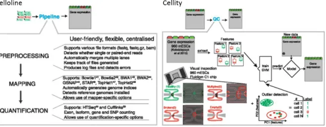
Celloline is one of the few quite generalized pipelines designed specifically for the early processing steps scRNA-seq data (Ilicic et al. 2016). It is a python pipeline that combines preprocessing, mapping and quantifying and has the capacity to process large datasets (see Figure 4). Currently supported mapping algorithms are bowtie, bowtie2, STAR, BWA, gsnap and salmon, and supported quantifying tools are tophat, htseq-count and cufflinks (https://github.com/Teichlab/celloline, 12/13/2017).
The output of celloline consists of two parts: gene expression matrix and read statistics matrix (Cells x Metrics), which can then be further analyzed e.g. with R-package cellity (https://github.com/Teichlab/cellity, 12/13/2017) which was developed together with celloline. Cellity contains the functionality for support vector machine (SVM) based quality classification of the cells.
2.4.2 Scater
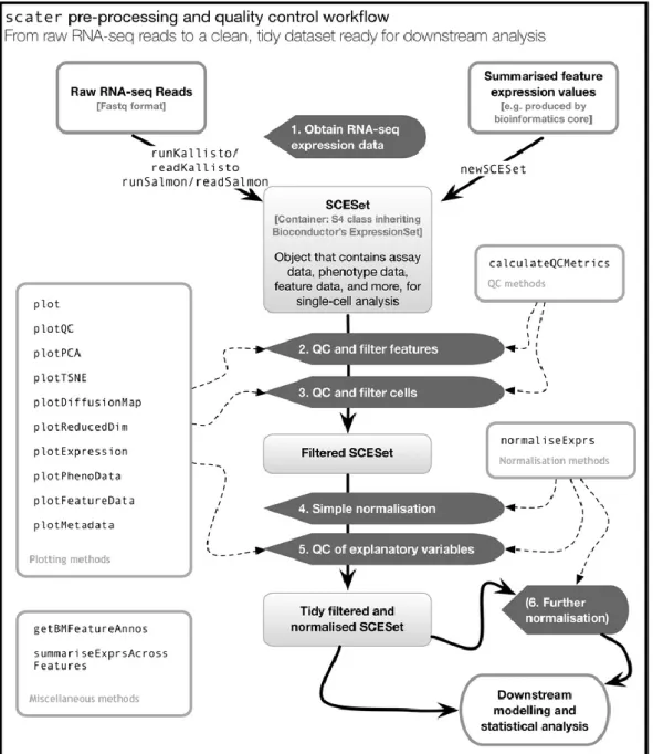
R/Bioconductor package scater is a recent tool that contains a platform and diverse set of functions for scRNA-seq data quality control, visualization and normalization (McCarthy et al. 2017). An overview of the functionality provided by scater is seen in Figure 5. Scater provides approaches to conduct all the most relevant steps in scRNA-seq preprocessing and monitoring data quality with the diverse plotting methods.
Figure 4: Classification and quality control of cells by celloline and cellity (Ilicic et al. 2016). The pipeline implemets the early processing steps for scRNA-seq data in a generalized approach, and the R-package cellity can then be used for quality control. Low-quality cells or reads are marked in red.
13
Especially useful are the functions for reading the data produced by Salmon and kallisto from list of directories, and summarize them all into one object. Scater even has the wrapper functions for running both Salmon and kallisto in R. The data is stored in a SingleCellExperimet (SCE) object (SingleCellExpressionSet/SCESet –class in earlier versions) which is specifically designed for scRNA-seq data, and transcript read counts can be easily summarized into gene counts within the workflow. Even though the package is built strongly compatible with the alignment-free methods, a new SCE-instance can be also built manually to store the quantification results of other approaches
Figure 5: Single-cell pre-processing and quality control with scater (McCarthy et al. 2017). The R-package provides diverse functions that can be combined into a single workflow. Note that SCESet-object is replaced by SingleCellExperiment-object in current version.
14
(http://bioconductor.org/packages/release/bioc/html/SingleCellExperiment.html,5/3/2018). Some additional metadata, for example annotations, can also be retrieved by scater.
After calculating diverse cell-specific and sample-specific QC-metrics (many of them being similar as defined by Ilicic et al 2016), uninterested features and low-quality cells can be filtered out. The features of interest may depend on the experiment, and should require case-by-case consideration. However, the genes that are constitutively silent across all cells i.e. systematic zeros is safe to drop already before normalization (Lun et al. 2016a).
Scater provides two main approaches for filtering low-quality cells. Outliers for a given metric (e.g. library size or proportion of mitochondrial RNA/spike-ins, mapping rate etc.) can be determined based on user-adjusted median-absolute deviation (MAD) thresholds. MAD is the average distance between each data point and the mean and describes the variation in a data set. Alternatively, an automatic outlier detection using multivariate normal methods can be used: basically, the principal component analysis (PCA) is applied for the given set of QC-metrics, and the outliers found by this approach should represent low-quality cells with abnormal library characteristics (McCarthy et al. 2017). Poor-quality cells may also sometimes form a second, distinct cluster (Stegle et al. 2015).
Scater provides some simple data normalization approaches (TPM, CPM, FPKM) for scaling normalization to remove biases caused by differences in sequencing depth, capture efficiency and other factors between samples, and batch effect correction (McCarthy et al. 2017). However, most scaling normalization methods are originally designed for bulk-RNA-seq data, and thus relying only to scater approaches may be insufficient. Scater is compatible with many tools specifically designed to account for scRNA-data normalization.
2.5
Normalization
Normalization refers to the scaling of the data so that the information of the samples can be reasonably compared as well as correcting uninformative biological and technical variation in data to ease the detection of interesting signals. Simple normalization for sequencing depth can be done e.g. by calculating TPM (Bacher & Kendziorski 2016). However, in addition to this kind of within-sample normalization, between-sample normalization is essential for downstream analysis.
Normalization has major effect on the interpretation of the data. When compared with bulk experiments, the contents of scRNA-seq matrix is heterogeneous and significantly sparser and noisier, which sets special challenges and makes the traditional normalization methods
15
potentially misleading, because the assumptions they make of the data are not necessarily valid (Bacher & Kendziorski 2016; Stegle et al. 2015; Vallejos et al. 2017). Regardless, the same methods are widely used (Vallejos et al. 2017). The challenging features of scRNA-seq data are next discussed more precisely, and some approaches designed to deal with them is then reviewed.
Sparsity i.e. the high proportion of zeros in expression matrix arises for both biological and technical reasons. For example, certain genes may not be expressed in different cell types or because of the transient states of the cells (Vallejos et al. 2017). Alternatively, it is possible to lose the signals of the genes that are actually expressed during the experiment: some transcripts may be lost e.g. in reverse transcription or PCR amplification phases, or in detection (Yuan et al. 2017). These are called dropout events.
The origins of noise are likewise various and their sources may be difficult to detect(Bacher & Kendziorski 2016; Vallejos et al. 2017). For example, when PCR-amplifying the scarce starting material obtained from each cell before sequencing, amplification biases may distort the original expression profile (Yuan et al. 2017). As a result, some transcripts that have optimal amplification properties may appear abundant and vice versa, even though their proportions were originally rather different. Experimental design, e.g. changes in culturing, capturing and sample preparation may lead in technical variation between cell populations, referred as batch effects (Stegle et al. 2015; Yuan et al. 2017). Sequencing platform may also produce certain lane effects.
2.5.1 Principles of global-scaling normalization
In short, global-scaling approaches are between-sample normalization methods that produce the normalized expression counts by dividing the raw read count of each cell by the estimated scaling factor (a.k.a. size factor) (Stegle et al. 2015; Vallejos et al. 2017). They are calculated with different methods depending on the normalization algorithm, and there is no consensus of the best approach (Vallejos et al. 2017). Even though being common approach in scRNA-seq, many global-scaling algorithms make assumptions that do not perform well with sparse scRNA-matrix, since the algorithms were originally developed for bulk RNA-seq. However, some scRNA-seq specific approaches have recently been developed, for example deconvolution based size factor calculation by Lun et al., which is described more precisely in chapter 2.5.2, and BASiCS (Bayesian Analysis of Single-Cell Sequencing data) (Vallejos, et al. 2015), which relies on spike-ins.
16
Vallejos et al. quite nicely visualized (Figure 6) and explained all the features affecting to the size factor sj in scRNA-seq experiments, and which ideally should be taken into account (Vallejos et al. 2017). For simplicity, only the homogeneous cell population is examined, even though the interpretation should be valid also for heterogeneous populations, assuming that most of the genes are not differentially expressed and the number of upregulated and downregulated genes is roughly equal.
As seen in Figure 6, the scaling factor sj should adjust for factors such as endogenous mRNA content of the cell (nj) depending from e.g. cell state before the lysis, the differing capture and RT efficiency (Fj) after the lysis and variability in amplification efficiency (Aj). Moreover, since a fixed number of reads are distributed between genes, the samples are subsequently diluted by a cell-specific factor Dj. Vallejos et al present two options to Dj interpretation. The first is library quantification (see equation 1),which aims to set the Dj so that a library contains the same number of molecules from each cell. In this case
𝐷𝑗 = 𝑚/(𝑛 𝑗 𝐹 𝑗 𝐴𝑗) (1)
where m is the desired number of molecules per cell. Without library quantification, Dj is the proportion of amplified molecules used to prepare the sequencing library. Finally, the sequencing depth i.e. the number of sequenced reads per molecule from each cell (Rj) varies stochastically.
Figure 6: Global scaling normalization for scRNA-seq data sets (Vallejos et al. 2017). Xij is a random variable representing the read count of a gene i in cell j. In order to normalize the expression levels, the scaling factor sj needs to be estimated for each cell.
17
2.5.2 Deconvolution-based scaling normalization and scran-package
As a result of the diverse nature of scRNA-seq experiments (i.e. several different platforms, whether or not spike-ins and/or UMIs are used etc.), it is hard to find a generalized method for normalization (Vallejos et al. 2017). Lun et al. aimed to develop a method that is not dependent on spike-ins and could be applied to all datasets (Lun et al. 2016a). This kind of method should recognize stochastic zeros that are found in actively expressed and thus informative genes due to sampling stochasticity, and semi-systematic zeros where the gene is silent only in certain cell sub-population(s) (Lun et al. 2016a). They developed a deconvolution method by combining the three commonly used scaling-normalization methods originally developed for bulk RNA-seq (DESeq, TMM and size factor normalization) and aiming to correct the assumptions that are not valid with scRNA-data. A visual description of the method is seen in Figure 7.
There are five key steps in the deconvolution method by Lun et al. First, a pool of cells is defined by clustering. Second, the expression values are summed across the pool. Third, the pool is normalized against an average reference built from the averaged expressions of the whole dataset. Next, the same is repeated to different pools of cells to construct a linear system. Finally, the pool-based size factors are deconvolved to their cell-based counterparts.
The method is available as a function in Bioconductor/R-package scran (http://bioconductor.org/packages/release/bioc/html/scran.html, 2/3/2018). Scran implements a
Figure 7: Deconvolution-based normalization (Lun et al. 2016a). Instead of using same size factor across the samples for scaling, the cells are first clustered and an optimal factor is calculated for each of the clusters with summing expression values (θi), normalizing against a reference cell and constructing linear system of equations. Cell-specific factors are finally deconvolved from the pool-based factors.
18
variety of low-level analyses of scRNA-seq data, such as normalization of cell-specific biases, assignment of cell cycle phase and detection of highly variable and significantly correlated genes.
2.5.3 Quantile-regression based normalization and SCnorm
Bacher et al. state that global-scaling approaches, also the ones designed to scRNA-seq data, are still insufficient to accommodate with the count–depth relationship in scRNA-seq data (Bacher et al. 2017). By this they refer to the systematic variation in the relationship between transcript-specific expression and sequencing depth. It cannot be explained accurately by a single scale factor common to all genes in a cell, since the relationship is not necessarily common across the genes. This is why scaling-factor normalization may lead to overcorrection for weakly and moderately expressed genes or undernormalization of highly expressed genes. To solve the problem, they developed novel between-sample normalization method SCnorm (https://bioconductor.org/packages/release/bioc/html/SCnorm.html, 2/3/2018) which uses quantile regression to estimate the dependence of transcript expression on sequencing depth for every gene. Genes with similar count-depth relationship are pooled, and the second quantile regression is used to estimate scale factors within each subgroup. Finally, the within-group adjustment for sequencing depth is performed using the estimated scale factors to provide normalized estimates of expression. In addition to this kind of between-sample normalization, SCnorm package also implements some within-sample normalization approaches to adjust for gene-specific biases.
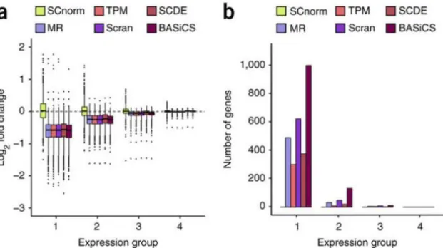
Bacher et al evaluated SCnorm by applying it for both simulated and real datasets, and the results were compared with five other normalization methods (see an example in Figure 8). Some remarkable differences were shown. According to the results, Bacher et al. suggest that the former normalization algorithms easily lead in false detections of DE-genes in downstream analysis. However, since the performance of any tool is typically affected by the properties of the data, the results may also vary. Bacher et al. recommend the usage especially with the data having groups with significantly differing counth-depth relationships. SCnorm-package contains a function plotCountDepth() for the visualization of this relationship in detected expression groups which can also be used in the evaluation of normalization results.
19
2.6
Confounding factors
Biological experiments always have sources of unwanted variation called confounding factors. Batch effects and other technical factors are most typical confounders, and depending on the biological interests of the experiment, also some biological factors may distort the interpretation of the data, if not taken into account (Stegle et al. 2015). For example, when detecting subpopulations in a heterogeneous tissue, the cells in differing stages of the cell cycle may affect the clustering, and thus the cell cycle effects are considered as confounders. On the other hand, experiments that aim to pseudotemporal ordering i.e. the construction of differentiation paths from a cell population, may consider cell cycle effect as a signal of interest (Bacher & Kendziorski 2016).
Chen & Zhou reviewed some statistical unsupervised and supervised methods recently developed to infer confounding factors (Chen & Zhou 2017). Supervised methods are application specific and restricted only to experiments where the primary variable of interest is known. An example of this kind of tool is OEFinder developed for Fluidigm C1 platform, which is designed to correct the expression variation correlated with capture sites with small or large plate output IDs, named as the ordering effect (OE) (Leng et al. 2016).
Figure 8: Log-fold changes (panel a) and numbers of DE-genes detected by MAST (panel b) after normalization by different tools (Bacher et al. 2017). In panel b, genes are divided into four equally sized expression groups based on their median among nonzero un-normalized expression measurements, and results are shown as a function of expression group.
20
Unsupervised methods are more generalizable and can be further divided into two subcategories (Chen & Zhou 2017). The first one includes approaches such as PCA and linear mixed models (LMM) which treat all genes similarly. In contrast, the methods of the second category divide the genes into a control set (consisting of e.g. spike-ins or certain cell cycle genes) and a targetset, which are treated differently. The confounding factors are inferred from the control set, which contains only genes known to be free of the effects of interest, and is then used to remove the confounding effects in the target set. An example of this kind of tool is scLVM (single-cell latent variable models) (Buettner et al. 2015). A recent tool scPLS (single cell partial least squares) by Chen & Zhou combines approaches from both categories of unsupervised methods.
In conclusion, due to the diverse nature of confounders and experiments, there is not any universal tool for the problem. For example scater-packagecan be usedforsimple batch effect correction, utilizing the PCA (McCarthy et al. 2017). Also scran package has a PCA-based function for de-noising the matrix. In PCA-based approach, the principal components of each gene in each sample are extracted to represent the confounding factors (Chen & Zhou 2017). These are then treated as covariates whose effects are further removed from gene expression levels. For more sophisticated methods, the tool to be used needs case-by-case consideration.
2.7
Obtaining biological insights
After normalization, the analysis flow is branched depending on what are the biological interests of the experiment and, what are the confounding factors. The goal may be e.g. cell type identification, cell type characterization or construction of gene regulatory networks, and Stegle et al. state that bulk RNA-seq tools can be generally used for these analyses (McCarthy et al. 2017; Stegle et al. 2015). There are also already several statistical methods and software tools developed for obtaining this kind of insights specifically from scRNA-seq data (see e.g. Table 1 in (Bacher & Kendziorski 2016)). Most of them assume that the data is already preprocessed and normalized, while some provide built-in normalization approaches.
21
The downstream analysis flow, e.g. cell-type identification presented in Figure 9 further consists of smaller tasks which can be completed in varying, and not necessary mutually exclusive approaches. In this chapter, couple of interesting applications that implement the downstream analysis flows are shortly discussed as a final part of the literature review.
A general issue in most downstream analyses is, that the high resolution of scRNA-seq experiments leads in high dimensionality e.g.number of features (rows) in expression matrix. Even though this kind of resolution is very powerful property for biological discovery, it comes with the cost called “curse of dimensionality” (Andrews & Hemberg 2018). The higher dimensionality, the harder to find significant differences between the samples i.e distinguish the differences between populations from the variability within a population. Moreover, the computational capacity needed to process the data is correlated with dimensionality. Feature selection i.e. dropping out the “uninformative” genes and dimensionality reduction i.e. projecting the data into a lower dimensional space by priorizing certain properties are main approaches to deal with the problem. According to Andrews&Hemberg, it is a common practise to apply several of them in a single analysis flow.
2.7.1 SC3: Cell type identification by consensus clustering
Identification of cell populations is an example of unsupervised clustering problem, which is one of the main fields in machine learning and also among the most popular goals of scRNA-sequencing (Andrews & Hemberg 2018). The amount of possibilities how to divide a large set of cells into different clusters is enormous, and in order to find a solution in a feasible time, all clustering algorithms make certain assumptions and approximations of the data. For example k-means clustering algorithm which is a part of SC3-method presented by Kiselev et al. Figure 9: Workflow for cell type identification after normalization (Andrews & Hemberg 2018). Feature selection for normalized expression matrix is followed by dimensionality reduction, distance calculation and clustering
22
assumes the clusters to be roughly similarly sized and spherical (Andrews & Hemberg 2018; Kiselev et al. 2017). Obviously, when a clustering algorithm is used for data that does not follow these assumptions, the result is not reliable, and thus there is no general solution for clustering. Several approaches are more precisely reviewed by Andrews&Hemberg.
K-means clustering looks for k clusters that are found based on k centroids i.e. points that represent the centers of each clusters. The first centroids are artificially picked, after which the algorithm iteratively calculates the average of the points that are near to each centroid, and sets these average values as the new centroids. When the centroids stay stable, the solution is found. Naturally, the clustering results may differ depending on how the original centroids were chosen. SC3 aims to increase the classification accuracy by consensus approach where k-means clustering is repeated several times and the outcomes are collected into a matrix which summarizes how often each pair of the cells is located into a same cluster (Kiselev et al. 2017). SC3 clustering by Kiselev et al. has five key steps: gene filtering, distance calculations (Euclidean, Pearson and Spearman), transformation of distance matrices, k-means clustering and computing a consensus matrix by cluster-based similarity partitioning algorithm (CSPA). Finally, the consensus matrix is clustered by hierarchical agglomerative clustering, and inferred into user-defined amount (k) of clusters. Each step has some adjustable parameters, which are, as default, set to the values found optimal by running the algorithm with six “gold-standard” datasets. According to Kiselev et al., these default values seemed to perform well when testing them with six additional public datasets, and finally, when applying it to a clinical data. SC3 is available as a Bioconductor/R package and is compatible with scater. Naturally, the increased classification approach comes with some computational cost, but computation can be sped up by parallelization.
2.7.2 Determining cell lineage and differentiation
In sequencing experiments, cells are potentially captured in unsynchronized stages of differentiation and cell cycle phases. This may be problematic for many scRNA-seq downstream analyses, but also enables insights that are not possible with bulk experiments. An example of novel downstream direction is pseudotemporal ordering i.e. computational reconstruction of cell differentiation path from the data, and also other dynamic cellular processes such as proliferation may be targets of interest (Bacher & Kendziorski 2016; Trapnell et al. 2014). When differentiation states of the cells are known, it is possible to e.g. predict the
23
dynamic genetic networks in larger scale biological processes such as organogenesis, repair and disease (Guo et al.2017).
The first remarkable method for determining differentiation pathways was Monocle by (Trapnell et al. 2014), and since then, several other approaches have been developed. According to Bacher & Kendziorski, most of them perform some type of dimensionality reduction followed by algorithms from graph theory, aiming to order cells so that the distance between them, determined by gene expression, is minimized. Guo et al. state that the methods that pseudotemporally classify cells based merely on transcriptome similarity require external knowledge, e.g. time information, cell identity or marker gene expression in order to determine the start and end points of dynamic processes, and thus cannot be always applied. As a solution, they developed a novel algorithm SLICE (Single Cell Lineage Inference Using Cell Expression Similarity and Entropy), which is based on the calculation of single-cell entropy (scEntropy) and the perception that the entropy inversely correlates with cell differentiation state (Guo et al. 2017). Recently, also (Teschendorff & Enver 2017) have confirmed the potential of entropy in studying cell differentiation.
Entropy can be seen as a measure of cellular heterogeneity: low entropy corresponds to narrow, well-defined gene expression patterns with strict regulatory constraints while high entropy corresponds to broad, diverse patterns of expression with weaker regulatory constraints (Guo et al. 2017). Thus, ‘entropy’ in this context refers to the multiple potentials or uncertainty in a biological system instead of e.g. the noise or disorder in gene expression. In short, SLICE calculates scEntropy by computing pairwise gene functional similarities based on Gene Ontology annotations, and then clusters the genes based on their functional similarity. These clusters are then used together with calculated expression similarity clusters to construct a cell network, in which the neighboring cells are grouped into cell clusters, and local minimums within individual cell clusters are identified as relatively stable cell states in the network. An R implementation of the algorithm can be found in https://github.com/xu-lab/SLICE.
24
3
Objectives
This thesis has three main objectives. First, gain insight of scRNA-seq analysis flow and especially find the optimal ways to preprocess the data and asses its quality. Second, test the relevant tools as the first phase of the computational part.Third and most importantly, construct an analysis pipeline by combining the best approaches and necessary quality metrics. The reliability of the pipeline should also be estimated, mainly by testing the pipeline with more than one publically available scRNA-seq datasets.
In this kind of experiment, where the pipeline is one of the main goals, a central issue is, how to define the “relevant” or “best” approaches for the pipeline. The amount of available tools for different data analysis steps is remarkable and is continuously increasing. Tools specifically designed to scRNA-seq experiments are picked whenever possible, since they are the major interest in this thesis. Moreover, since the experimental standards are not established, the methods that are not strictly dependent on spike-ins or UMIs is preferred over the more specific methods. Finally, the compatibility between the tools in different phases should be taken into account.
In the scope of this thesis, there are clearly limited resources for comprehensive testing and comparison of several tools with various parameters in different phases of the analysis flow. Thus, the “best approach” that is finally chosen into the pipeline does not necessarily mean that it is the best method of all available approaches. Instead, it may be for example a familiar, commonly used tool (e.g. FASTQC), or a tool that seems to have some favorable or interesting properties either in general or in single-cell specific point of view. For interested readers, the comparison and validation of different tools are discussed broadly and more systematically in other research articles already available or in press.
25
4
Materials and methods
4.1
Data
The two publically availablescRNA-seq datasets used for building and testing the pipeline are presented in Table 2. The data was accessed through NCBI archive (https://www.ncbi.nlm.nih.gov/gds/). Only parts of the full Camp dataset consisting of 770 samples was used, while all 466 samples in Darmanis dataset was originally loaded. However, one of the Darmanis samples had a truncated fastq-file and was thus excluded from further analysis.
Table 2: Properties of the used data. Source organism for both datasets is Homo sapiens. Name Tissue Accession Cell types Samples Article
Darmanis Brain GSE67835 9 465 Darmanis et al. 2015
Camp Liver GSE81252 4 247 Camp et al. 2017
Gencode sequences of release 27 was used as reference transcriptome ftp://ftp.ebi.ac.uk/pub/databases/gencode /Gencode_human/release_27, 11/6/2017). The transcriptome file containing only protein-coding sequences (gencode.v27.pc_transcripts.fa) was preferred over the full set of transcripts (gencode.v27.transcripts.fa). An alternative reference containing also spike-in RNA sequences was constructed by concatenating the sequences of a common set of external RNA controls developed by the External RNA Controls Consortium (ERCC) with the transcript file. These ERCC-sequences can be downloaded from https://tools.thermofisher.com/content/sfs/manuals/ERCC92.zip.
4.2
Environment and the relevant tools
Computational environment and capacity was provided by CSC – IT Center for Science, Finland (https://www.csc.fi/), and the work was done in Taito-supercluster. The resource management system SLURM used by Taito (https://research.csc.fi/taito-batch-jobs, 4/10/2018) affected slightly into the structure of the pipeline and may thus also affect the portability. Many of the tools discussed in literature review were also included into final pipeline. Table 3 presents the tested and chosen tools together with the reasoning. When designing the data-analysis steps, especially the step-by-step workflow presented by Lun et al. together with the course material by Hemberg lab provided solid base to build on (Lun et al. 2016b; https://hemberg-lab.github.io/scRNA.seq.course/ 4/19/2018).