D
S
E
Working
Paper
A generalized Dynamic
Conditional Correlation
model for portfolio risk
evaluation
Monica Billio
Massimiliano Caporin
Dipartimento
Scienze Economiche
Department
of Economics
Ca’ Foscari
University of
W o r k i n g P a p e r s D e p a r t m e n t o f E c o n o m i c s C a ’ F o s c a r i U n i v e r s i t y o f V e n i c e N o . 5 3 / W P / 2 0 0 6
ISSN 1827-336X
The Working Paper Series is availble only on line (www.dse.unive.it/pubblicazioni) For editorial correspondence, please contact: [email protected]
Department of Economics Ca’ Foscari University of Venice Cannaregio 873, Fondamenta San Giobbe 30121 Venice Italy
Fax: ++39 041 2349210
A generalized Dynamic Conditional Correlation model
for portfolio risk evaluation
Monica Billio
University of Venice
Massimiliano Caporin
University of Padova
Abstract
We propose a generalization of the Dynamic Conditional Correlation multivariate GARCH model of Engle (2002) and of the Asymmetric Dynamic Conditional Correlation model of Cappiello et al. (2006). The model we propose introduces a block structure in parameter matrices that allows for interdependence with a reduced number of parameters. Our model nests the Flexible Dynamic Conditional Correlation model of Billio et al. (2006) and is named Quadratic Flexible Dynamic Conditional Correlation Multivariate GARCH. In the paper, we provide conditions for positive definiteness of the conditional correlations. We also present an empirical application to the Italian stock market comparing alternative correlation models for portfolio risk evaluation.
Keywords
Dynamic correlations, Block-structures, Flexible correlation models
JEL Codes C51, C32, G18
Address for correspondence:
Monica Billio Department of Economics Ca’ Foscari University of Venice Cannaregio 873, Fondamenta S.Giobbe 30121 Venezia - Italy Phone: (++39) 041 2349170 Fax: (++39) 041 2349176 e-mail: [email protected]
his Working Paper is published under the auspices of the Department of Economics of the Ca’ Foscari University of Venice. Opinions expressed herein are those of the authors and not those of the Department. The Working Paper series is designed to divulge preliminary or incomplete work, circulated to favour discussion and comments. Citation of this paper should consider its provisional character.
1
Introduction
In the last few years, the empirical and theoretical analysis concerning multi-variate GARCH models attracted a growing interest for two main reasons: the availability of more and more powerful computers that enabled the estimation of complex models with an elevate number of parameters and the introduction of a new class of models: the Dynamic Conditional Correlation multivariate GARCH (DCC) by Engle (2002). Several generalizations of the Engle’s model as been proposed (among others Cappiello et al. 2006, and Franses and Hafner, 2003, Billio et al., 2006) and some theoretical studies have also been developed (McAleer et al., 2006). These papers focused both on the developments of new parameterizations and on their use in empirical applications, demonstrating an high capability to adapt to practical problems.
In this paper we introduce a new DCC-type model that generalized the Flex-ible DCC of Billio et al. (2006), FDCC. We start from the empirical evidence that in asset allocation problems we need flexible and feasible models to con-struct optimal portfolios. Asset managers generally invest by differentiating their portfolio by area, branches or sectors and type of instruments. This fact suggests to develop the block structure in the parameters of the FDCC model, thus allowing for constant dynamics only among block of assets belonging to the same category. Our model generalizes the FDCC structure by allowing for possible interactions in the correlation dynamics among classes of assets.
In Section 2 we review current DCC type models and in section 3 we in-troduce the Quadratic FDCC model also providing conditions for positive defi-niteness and stationarity. Section 3 reports an empirical example based on the sectorial indices of the Italian Stock Market (MIBTEL). Section 4 concludes.
2
Modeling Dynamic Conditional Correlations
The starting point for the analysis of dynamic correlation models is the Con-stant Condition Correlation model of Bollerslev (1991). In his paper, Bollerslev assumed that the variance-covariance matrix ofεt (a K-dimension set of asset
returns) could be factorized as follows:
Ht=DtRDt (1)
whereRis a correlation matrix andDtis a diagonal matrix of conditional
volatil-ities. For the sake of exposition we assume that the mean is not relevant. For each series a GARCH-type model could be fitted for estimating the conditional variance without any constraint on a common structure. Each conditional vari-ance could be modelled with a standard GARCH model or with more advvari-anced parameterisations such as GARCH models with asymmetry effects as in Glosten et al. (1993) and in Caporin and McAleer (2006), or EGARCH representations as in Nelson (1991).
The representation with constant conditional correlations allows for a two-step estimation procedure: at first, we estimate the conditional variances, which can then be filtered out by premultiplying εt by D
−1
t ; then, the correlation
matrix can be estimated. Furthermore, we can estimate the correlation with the simple sample estimator
R=D −1 t εtε′tD −1 t T (2)
Unfortunately, the assumption of constant correlations is really questionable. In fact, it is well-known that correlations are not stable over long periods. Engle (2002) introduced a limited dynamics into the correlations in order to overcome this limitation. Engle restated the decomposition (1) as:
Ht=DtRtDt (3) Rt= (Q ∗ t) −1 Qt(Q ∗ t) −1
where he assumed that the time-dependent correlation has a quadratic structure (which was added to ensure that we have, at the end, a correlation matrix). Furthermore,Qthas the following expression
Qt= [1−α(1)−β(1)] Γ +α(L)ηt−1η
′
t−1+β(L)Qt−1
where: ηt=D−1
t εt; the polynomial parameters are defined asα(L) =qi=1αiLi,
β(L) =pi=1βiLiand must satisfyα(1) +β(1)<1in order to rule out
explo-sive patterns andΓ =T−1T i=1ηtη
′
tis the unconditional (sample) correlation
matrix. The dynamics is thus very similar to a GARCH-type equation. Further-more, the unconditional correlations are equal to the sample correlations (i.e. unconditionallyQ = [1−α(1)−β(1)] Γ +α(L)Q+β(L)Q=⇒Q= R = Γ
); we will refer to this result as the ”correlation targeting” property. Finally,
Q∗
t =diag(√q11,t,√q22,t, ...√qnn,t).
A very similar approach is included in the paper of Tse and Tsui (2002), the only difference is in the termηt−1η
′
t−1which is substituted by a short term
correlation estimatem−1m
j=1ηt−jη ′
t−j withm≥K.
This model is clearly parsimonious since it requires just two parameters to introduce dynamics into correlations. However, it implies several strong restric-tions: first, there is no interdependence among variances, among correlations and between variances and correlations; second, the dynamics is constant over all correlations.
We can solve the first point only moving from the DCC model to stan-dard multivariate GARCH models like the Vech or the BEKK of Engle and Kroner (1995). These two models allow for interdependence among variances and covariances and thus they implicitly assume dynamic correlations, even if their focus being on dynamic covariances. Unfortunately, BEKK and Vech models are useless in systems with more that 4 or 5 variables since they have
serious optimization problems leading to unstable and inconsistent parameter estimates. Differently, the empirical interest is in models with many assets, possibly more than 100. One solution is then to split the problem, estimating conditional variances on a univariate basis and focusing in a second step on the correlations. Clearly, the use of a two-step approach provides important compu-tational advantages, but it excludes any direct interaction among covariances. The introduction of lagged cross-sectional dependence between the variances could follow standard models, as the VARMA-GARCH of Ling and McAleer (2003). We will not directly address this issue since the focus of the paper is on correlation modelling. Anyway, we underline that the correct specification of the variance dynamics is fundamental. In fact, the dynamic evolution of the correlation could be influenced by a possible misspecification of the variance equations. We thus face a trade-off between the use of an advanced and possibly multivariate specification of the variance evolution and the model feasibility.
Within the dynamic correlation literature, the most common approach con-siders univariate specification of the variances, possibly including asymmetric terms following the GJR model of Glosten et al. (1993). In the empirical appli-cation we will follow this strategy.
The second limitation, given by the constancy of the dynamics over all the correlations, has been already addressed in the econometric literature. The DCC model was generalized by Engle (2002), who suggested the following Generalized DCC trying to solve the constraint of equal dynamics for all correlations
Qt= [ii′−A−B]◦Γ +A◦ηt−1η
′
t−1+B◦Qt−1 (4)
where ◦is the Hadamard product (elementwise matrix multiplication),A and
B are square matrices and positive definiteness is guaranteed by their positive definiteness (see Ding and Engle, 2001). This model solved one of the draw-back of the original DCC but, unfortunately, the number of parameters greatly increases and makes the model empirically unattractive.
Additional extensions shortly appeared in the literature:
i) Cappiello et al. (2006) provide a different extension of the DCC model by introducing asymmetry in the correlation dynamics and translating the model into a quadratic form
Qt= Γ−A′ ΓA−B′ ΓB−G′¯ F G+A′ ηt−1η ′ t−1A+B ′ Qt−1B+G ′ ξt−1ξ ′ t−1G (5) where ξt = I(ξt<0)◦ξt, A, B, G are diagonal parameter matrices, Γ
is again the sample covariance matrix of the standardized residuals and F¯ is the sample covariance matrix ofξt; this model adds flexibility to the previous one, however the number of parameters increases with system dimension and the positive definiteness is obtained by constraining the matrix Q¯−A′¯
QA−
B′¯
QB−G′¯
ii) Franses and Hafner (2003) suggested another Generalized DCC model Qt= 1− n i=1 αi−β Γ +αα′ ◦ηt−1η ′ t−1+βQt−1 (6)
with α being a vector of dimension n. Here the positive definiteness is guaranteed without constraints but the correlation targeting property is no more valid;
iii) McAleer et al. (2006) generalize the model providing a representation in which all the dynamic correlations can have a different dynamic pattern; their approach is particularly useful from a theoretical point of view, since it provides regularity conditions for the moments and the asymptotic properties of the quasi maximum likelihood estimator applied to dynamic correlation models (and the DCC models of Engle (2002) are special cases);
iv) Billio et al. (2006) suggest two special cases of the Generalized DCC of Engle (2002) and Franses and Hafner (2003), by requiring that the parameter matrices or parameter vectors is partitioned. The intuition behind this choice is that the dynamics cannot be common for all correlations but a too generalized parameterization is not feasible; therefore, they suggest to group variables in coherent sets mirroring the empirical needs of sectorial or geographical asset allocation (i.e. stocks from Europe and Asia or belonging to the Energy and Financial sectors); in formula (4), they required that
A= αi,11i(m1)i(m1) ′ αi,12i(m1)i(m2) ′ · · · αi,w1i(m1)i(mw) ′ αi,12i(m2)i(m1) ′ αi,22i(m2)i(m2) ′ αi,w2i(m2)i(mw) ′ .. . . .. ... αi,w1i(mw)i(m1) ′ αi,w2i(mw)i(m2) ′ · · · αi,wwi(mw)i(mw) ′ (7) wherem1, m2, ...mware the number of assets in each group (similarly forB); in
that case the correlation matrix is positive definite if so is the matrix[ii′
−A−B]◦
Γ; the constraints are heavy but feasible if off-diagonal blocks are filled up with zeros (i.e. onlyαi,jj = 0); they named this particular DCC the Block-Diagonal
DCC (BDDCC) model. To solve this further limitation they generalize the model of Franses and Hafner (2003) adding the constant
Qt=cc ′ ◦Γ +αα′ ◦ηt−1η ′ t−1+ββ ′ ◦Qt−1 (8)
and requiring the parameter vectors to be partitioned vectors, asα={α1, α1, α1, α1, α2, α2, α3, α3, α3,};
in that case they gain the positive definiteness but loose, in general, the correla-tion targeting property, as in the Franses and Hafner (2003) model. Differently from their approach, Billio et al. (2006) can impose positive definiteness with the following constraintsαiαj+βiβj+cicj = 1fori, j= 1...n; they labeled this
model the Flexible DCC; in both cases the parameters of the GARCH part (not the constant) must satisfy a ”stationarity” constraintαiαj+βiβj <1. McAleer
(2005) and Bauwens et al. (2006) provide an extensive survey on multivariate correlation models.
3
The Quadratic Flexible DCC Model
In this paper we introduce a new DCC-type mode which generalize the Flexible DCC: the Quadratic Flexible DCC can be also considered a special case of the Asymmetric DCC of Engle, Cappiello and Sheppard (2006). We suggest the following parameterization ofQt: Qt=C′ΓC+A′ηt−1η ′ t−1A+B ′ Qt−1B (9)
whereA,B andCare symmetric matrices. This model nests the FDCC which correspond to a Quadratic FDCC with diagonal partitioned parameter matrices. As the FDCC this model generally looses the correlation targeting property which can however be imposed with a set of restrictions. The quadratic structure of the model guarantees the positive definiteness ofQt, given a suitable starting
point. A comment on parameter constraint is worthwhile: in standard DCC theα and β parameters must satisfy a constraint (α+β < 1) that rules out explosive correlation patterns; the QFDCC model requires a similar constraint but it must be imposed on the eigenvalues ofA+B. In fact, the QFDCC can be thought as a particular BEKK model once the variance effect has been filtered out. Then, following Engle and Kroner (1995) we can recast the QFDCC in a companionV ech-type form and use their Proposition 2.7. Consequently, the QFDCC model provides stationary correlations if: i)C′ΓC is positive definite;
ii) the eigenvalues ofA+B are in modulus less than 1.
In the QFDCC model we can adapt block structures to the parameter ma-trices as in (7). Finally, by removing the assumption of diagonal parameter matrices, as in the Asymmetric DCC, the QFDCC model allows for interdepen-dence among correlations. Clearly, a completely unrestricted model is unfeasible from an estimation point of view. For this reason, we suggest several special cases: with diagonal parameter matrices as in the A-DCC (5); with partitioned diagonal matrices, similarly to the FDCC (8); finally, block-partitioned repre-sentations could be adopted as in BDDCC (7 ). We present a particular example for this last case.
Assume that we are considering a system with K = 5 assets grouped into two sets ofn1 = 3 and n2 = 2 assets, respectively. Also assume the following
structures for the parameter matrices
A = 0 0 0 a2 a2 0 0 0 a2 a2 0 0 0 a2 a2 a2 a2 a2 a1 0 a2 a2 a2 0 a1 B= 0 0 0 b2 b2 0 0 0 b2 b2 0 0 0 b2 b2 b2 b2 b2 b1 0 b2 b2 b2 0 b1 (10) C = 1 0 0 c2 c2 0 1 0 c2 c2 0 0 1 c2 c2 c2 c2 c2 c1 0 c2 c2 c2 0 c1
Then, by substitution on (9) we can verify that: i) the interdependence between correlations can be handled with a very limited number of parameters; i) the QFDCC model allows the combination of constant correlations for some assets and dynamic correlations for others (simply imposing the restrictionsc2=b2=
a2 = 0). Furthermore, we can estimated a generalized model and run some
likelihood ratio test for nested models. Finally, the QFDCC can be generalized adding asymmetry terms following the strategy proposed by Cappiello et al. (2006).
3.1
Estimation and Testing
Maximum likelihood is the standard tool for the estimation of dynamic condi-tional correlation models presented in this work. Following Engle (2002), letθ1
be the parameter set of the univariate GARCH models andθ2 the parameter
set of the dynamic correlation structure. We can represent the likelihood of the model as follows: LogL(θ1, θ2|Xt) =− 1 2 T t=1 klog (2π) + log (|Ht|) +εtH −1 t ε ′ t (11)
Further, exploiting the relation (3) we can write:
LogL(θ1, θ2|Xt) =− 1 2 T t=1
klog (2π) + log (Rt) + 2 log (|Dt|) +εtD
−1 t R −1 t D −1 t ε ′ t (12) Engle suggested a first estimation stage where the correlation matrix has to be replaced by an identity matrix
LogL(θ1|Xt) =− 1 2 T t=1
klog (2π) + log (In) + 2 log (|Dt|) +εtD−t1I
−1 n D −1 t ε ′ t (13) This step is equivalent to univariate estimation of GARCH models. In a second step, conditionally on the parameters estimated in the first step, we have the following log-likelihood LogLθ2|ˆθ1, Xt =−12 T t=1
klog (2π) + log (Rt) + 2 log (|Dt|) +ηtR
−1 t η ′ t (14) whereηt=D−1
t εt are the first stage standardized residuals.
According to the results of Comte and Lieberman (2003), Ling and McAleer (2003) and McAleer et al. (2006), the maximum likelihood estimators are con-sistent and asymptotically normally distributed.
Given the relations between Engle’s DCC, the Flexible DCC and the Quadratic FDCC model we can apply several likelihood tests for parameter restrictions. The LR tests have an asymptotic chi-square distribution under the assump-tions and regularity condiassump-tions stated in Comte and Lieberman (2003), Ling
and McAleer (2003) and McAleer et al. (2006). We stress that our working hy-pothesis will never be an unrestricted QFDCC, which is not feasible, but instead we consider the Block QFDCC (with block partitioned parameter matrices). In order to evidence all the possible bivariate model comparison we consider the two-block example. In that case,A is defined as follows
A= a1in1i ′ n1 a12in1i ′ n2 a12in2i ′ n1 a2in2i ′ n2 = A1 A′12 A12 A2 ,
and similarlyBandC. We can then test the block structured benchmark model against a set of alternative parameterizations:
i) Block QFDCC against Block Diagonal QFDCC: this is obtained by re-stricting to 0 all off-block diagonal coefficients,a12=b12=c12= 0;
ii) the benchmark model with respect to a structure with diagonal blocks restricted to be diagonal: in that case, we assume that the correlations belonging to a given diagonal block have no feedback effects (that is, they are simply characterized by the same dynamic behavior): in that case we impose A1 =
a1In1, and similar representations are used forA2, B1, B2, C1, C2;
iii) Block QFDCC against a Diagonal QFDCC: this is the restriction that implies an FDCC model where there is no interdependence across correlations; this is equivalent to merging restrictions i) and ii);
iv) our benchmark model can be also compared to Engle’s DCC model; this is equivalent to the following set of restrictions: A1 = A2 = aIn1+n2,
B1 =B2 =bIn1+n2, (similar to i) and ii) but excluding the constant termC),
c1=c2=
√
1−a2−b2(given that we are using a quadratic form), andc12= 0;
v) a CCC model, that isA=B= 0andC=In.
Additional restrictions could be considered for testing mixed models such as the one proposed in (10). In addition, the information criteria can be used to compare the QFDCC with non-nested models like the Franses and Hafner DCC.
4
Portfolio Risk Evaluation with DCC-type
mod-els
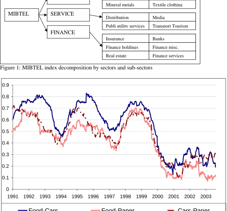
Dynamic correlation models may provide useful insights in several financial ap-plications including asset allocation within a Markowitz approach, forecast eval-uation analysis and portfolio risk evaleval-uation. In this paper we focus on this last case using a set of stock market indices. In details, we consider the main Italian stock market index, the Mibtel, and its sectorial decomposition which we report in Table 1.
[INSERT Figure 1 - Mibtel sectorial decomposition]
The data were downloaded from Datastream and cover the range January 1991 to September 2003 at the daily frequency. The index has two levels of
disaggregation. In the first, the index is decomposed in three main groups In-dustrial, Service and Finance. These three indices are further disaggregated into a group of 20 sub-sectors. The whole sample consists of about 3400 observa-tions. Following a standard practice, we fitted univariate GARCH models with asymmetry following Glosten et al. (1997) on the log-returns of the sub-sector indices. Table 2 reports the estimated parameters and the quasi maximum like-lihood standard errors. All sub-sectors conditional variances show a relevant asymmetric effect and only three reports a GARCH coefficient lower than 0.7. Given the comments reported in section 2 and the focus on correlation dynamics, we did not consider further GARCH specifications.
[INSERT Table 1 - Univariate GARCH estimates]
Following the approach of Engle (2002), after the estimate of the conditional variance models, we compute the standardized residuals. On the resulting series we fit then dynamic correlation models. As benchmark model we computed the sample (unconditional) correlation matrix on the standardized residuals. This estimate is equivalent to a Constant Conditional Correlation model. In this case the correlation model likelihood is equal to -9842.368.
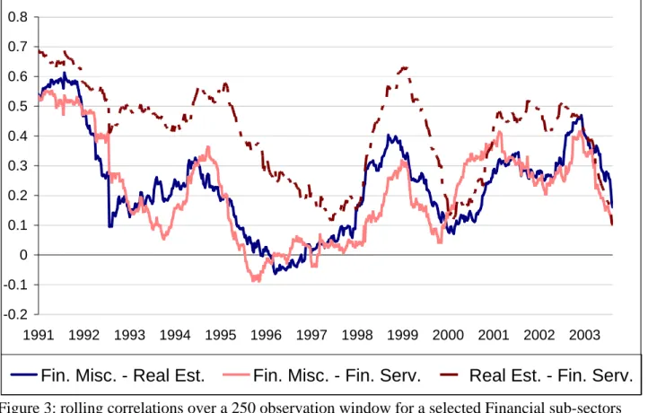
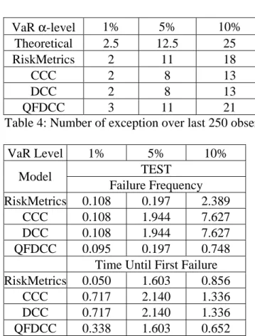
We also computed the unconditional correlations (again on the standard-ized residuals) using a rolling window of 250 observations. Some patterns are reported in Figures 1 and 2. This graphical analysis evidences that correlations are not stable over time and, more interestingly, that correlations show similar patterns between sub-sectors groups.
[Insert Figures 2 and 3- rolling correlations]
This graphical analysis suggests that the QFDCC should be considered as a valid alternative to the excessively restricted DCC and CCC representations. Tables 2 and 3 reports parameters estimates for the whole sample for DCC and for the diagonal QFDCC models. The log-likelihoods suggest that the QFDCC model should be preferred to the DCC (it provides a small but signifi-cant increase in the likelihood). However, the improvements achieved with the QFDCC (and only with a diagonal representation) are very relevant, suggesting that even small increases in model flexibility may provide valid and preferred representations. Standard likelihood ratio tests strongly support these findings.
[INSERT Table 2and 3 parameter estimates of DCC and QFDCC]
Our final purpose is to compare the performances of CCC, DCC and QFDCC in evaluating portfolio risk. For this reason, we focus on the last two years of our sample and we estimate the various models in a rolling window of 250 ob-servations and a step of 10 obob-servations. This correspond roughly to a portfolio allocation and evaluation which is updated every two weeks. In order to get directly comparable portfolios in term of returns and avoid any discussion on
the estimation of mean expected returns, we consider equally weighted portfo-lios (i.e. the 5% of the global portfolio is invested in each of the 20 sub-sectors indices of the Mibtel). The various portfolios are then equivalent in terms of returns but not in their exposition to market risk which is influenced by the sec-ond order moments. We compare the correlation models using the Value-at-Risk measure with a backtesting procedure.
The VaR is the quantile of portfolio returns (rt) satisfying
V aR(t,α)
−∞
rtf(rt)drt=α. (15)
The backtesting analysis considers a comparison over the last 250 days and focuses mainly on exceptions: i.e. the number of cases in which the portfolio returns underperform the VaR measure. In that case, we also computed the RiskMetrics model (RM) (JP Morgan, 1996), which is the alternative bench-mark model extremely popular in the literature. The RM model considers that variances and correlations follow an exponentially weighted moving average. Define the returns on a sub-sector index asri,t, denote the variance-covariance
matrix of the 20 indices byΣt, and letωbe the row-vector of portfolio weights
(each element of the vector is equal to 1/20 (we are considering an equally weighted portfolio). Then, time varying portfolio returns are:
rt=ω r1,t r2,t .. . r20,t (16)
while portfolio variances are:
σ2t=ωΣtω′. (17)
Note that portfolio weights are repositioned at the equally weighted level every 10 days while the variance-covariance matrix is estimated with a CCC (i.e. with constant correlations), a DCC, a QFDCC and finally with the RiskMetrics model. In this last case, we estimate the elements of Σt using the recursive
formula
σi,tσj,t=λσi,tσj,t+ (1−λ)ri,trj,t i, j= 1...20 (18)
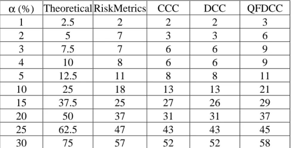
andλset to0.97. Table 4 reports the exceptions realized by the three correlation models and by the RM.
[Table 4 - exceptions]
Among the various models, only the QFDCC and the RM models provide an exception number very close to the theoretical value. Differently, CCC and DCC report the same result, which is too conservative. They provide a lower exception number, which indicates that the portfolio variances provided by these
two approaches are larger than the one provided by RM and QFDCC. This fact is not negative if our final purpose is to adequately cover market risk exposure. However, a more conservative VaR methodology necessarily implies a larger opportunity cost: larger VaR is equivalent to a larger amount of immobilized resources.
A comparison between correlation models cannot be based only on counting the exceptions, but further metric must be considered. The literature focuses on two standard approaches: testing for VaR model failures, following Kupiec (1995); comparing models with loss functions, following Lopez (1998). In this paper we combine these standard techniques with some additional measures proposed in Caporin (2003). Kupiec (1995) suggests two tests for the evalua-tion of VaR measures: the Proporevalua-tion of Failure test and the Test Until First Failure. Both tests are based on the assumption that exceptions follow a bi-nomial distribution and are asymptotically distributed as a chi-square variable with one degree of freedom. Both tests are used to verify the null hypothesis that VaR measures are correctly specified. Table 7 reports the tests for the various correlation models.
[Table 5 - tests for VaR]
Even in this case, the CCC and DCC models provide the worst results: larger test statistics, closer to the rejection area; rejection of the null hypothesis in the 10% VaR case; finally, the tests allow to infer that the two models provide exactly the same exceptions. Differently, RM and QFDCC provide comparable test statistics.
Unfortunately, it is well-know that these tests have limited power in distin-guishing among various models for VaR, see among other Lopez (1998). Loss functions represents an alternative approach that can be used to compare VaR models. These loss functions can be appropriately designed in order to overcome the tests limitations. Lopez (1998) suggests a loss function based on regulatory needs: LfL= T t=1 1 + (rt−V aRt)2 It(rt< V aRt) (19)
whereIt is an indicator function that selects exceptions. This loss function
pe-nalizes the VaR models that provide largest losses at the exceptions. However, a bank would prefer a VaR model that: (i) satisfy Basel Accord requirements, (ii) reduces losses at the exceptions, (iii) and also reduces the opportunity cost of VaR (the VaR also measures the amount of money that a financial institutions must immobilize to cover market risk exposure). A VaR model that satisfies points i) and ii) and that provides lower bounds than the other is clearly pre-ferred, since it translates in lower immobilization of liquidity resources).
Lopez loss function focus only on point (i); additional metrics are therefore needed. Caporin (2003) introduces alternative loss functions that can be used to compare models in terms of (ii) and (iii). The loss functions focus on the distances between the VaR bounds and the realized portfolio returns. Therefore
they can be used on the whole return path and not only on the exceptions. We report here two loss functions, that can be thought as first and second order losses LfF = T t=1 |rt| − |V aRt| |V aRt| (20) LfS = T t=1 (|rt| − |V aRt|)2 |V aRt| (21) LfC=LfF+LfS. (22)
[Table 6 - loss functions]
If the attention is given only to the exceptions, then the Lopez loss function should be used. In that case, the RM model provide the best result at the 1% level, while the optimal model is the DCC at the 5% and 10% Value-at-Risk level; at the opposite, the QFDCC is the worst case. This in turn implies that, at the exceptions, the QFDCC provide a lower portfolio variance compared to the other models; it is less conservative than the other models and this give rise to larger losses. If we move from the exception cases to the whole path of the portfolio variances, we should consider the alternative loss functions previously introduced. These loss functions have been calculated over the full back-testing period and not only over the exceptions. In that case, we note that the result is completely reversed: the QFDCC model is the optimal choice at 1% and 5% cases while the RM is the best model for a 10% VaR. Collecting these results we can state the following: regulators should prefer a Lopez loss function approach for comparing VaR models while financial institutions should push for the use of different loss functions. In fact, a more flexible approach which satisfies the Basel Accord Requirements and provides lower VaR bounds could reduces the opportunity cost of immobilizing resources.
Finally, we consider a further analysis on VaR bounds using correlations among them and awe also compare the VaR levels at various quantiles. The purpose of this additional analysis is to verify if the correlation models we con-sidered provide VaR bounds close one to the other. A high correlation between two sequences of exceptions suggest that the two models detect the very same VaR exceptions. Similarly, a high correlation between VaR bounds evidences that the proposed models provide similar portfolio variance dynamics. Table 7 reports the correlations among VaR bounds and among the sequences of excep-tions at 1%, 5% and 10% VaR, respectively.
[Table 7 correlations]
It clearly emerges that: CCC and DCC models provide the same exceptions as we previously noted; QFDCC model is close to the DCC one; and, finally, that the RM model is far from the DCC-type models, in particular at 1% and 5% VaR levels.
Finally, table 8 reports the VaR exceptions at various quantiles, from 1% to 30%, together with the theoretical exception values. We can note that all the models are much more conservative increasing the quantile probability.
[Table 8 quantiles and exceptions]
Summarizing our findings, we can state that the QFDCC model provides a significant increase in the log-likelihood compared to standard alterative cor-relation models. Furthermore, if the comparison is based on a portfolio risk evaluation framework, the QFDCC model produces exceptions closer to the theoretical values. Finally, using loss functions we verify that the CCC and DCC models generally provide wider VaR bounds that satisfy Basel Accord requirements but also imply a higher opportunity cost.
5
Conclusions
This paper introduces a new dynamic conditional correlation model, the Quadratic Flexible DCC, that generalizes the DCC model of Engle (2002) and the FDCC model of Billio et al. (2006). The model allows for interaction among corre-lations with a quadratic structure similar to the one included in the BEKK-GARCH model of Engle and Kroner (1995). Furthermore, differently from the DCC, a constant is included to guarantee more flexibility. Finally, the param-eters are imposed to be constant across clusters of assets that can be defined a priori.
Following this approach, the parameter number greatly reduces and parame-ter matrices become partitioned matrices. The use of block-structure parameparame-ter matrices provides relevant advantages and a limited increase in model complex-ity. The proposed approach could be used in most multivariate GARCH models, including the BEKK of Engle and Kroner (1995), and in most of the parameter-izations described in McAleer (2005) and Bauwens et al. (2006). Furthermore, the use of block-structures and quadratic forms could also be considered within a multivariate stochastic volatility framework extending the models presented by Asai et al. (2006).
The QFDCC model is designed to be used in empirical finance applications involving asset management and risk evaluation. This paper provided an empiri-cal analysis in this second area, considering the VaR computation with different approaches, including CCC, DCC, QFDCC and the RiskMetrics models. In that particular case, the QFDCC model provides the best results on most cases providing a number of exceptions in line with Basel Accord requirements and a narrower VaR bounds.
References
[1] Asai, M., M. McAleer and J. Yu, 2006, Multivariate stochastic volatility: a review, Econometric Reviews, 25, 145-175
[2] Bauwens L., S. Laurent and J.K.V. Rombouts, 2006, Multivariate GARCH models: a survey, Journal of Applied Econometrics, 21, 79-109
[3] Billio, M., M. Caporin and M. Gobbo, 2006, Flexible dynamic conditional correlation multivariate GARCH for asset allocation, Applied Financial Economics Letters, 2, 123-130
[4] Bollerslev T., 1990, Modelling the coherence in short-run nominal exchang-erates: a multivariate generalized ARCH approach, Review of Economic Studies, 72, 498-505
[5] Caporin, M., 2003, Comparing Value-at-Risk measures in presence of long memory conditional variances, GRETA Working Paper, proceedings of the ASSET 2002 Conference, Cyprus, November 2002.
[6] Caporin, M. and M. McAleer, 2006, Dynamic Asymmetric GARCH, Jour-nal of Financial Econometrics, 4(3), 385-412
[7] Cappiello L., R.F. Engle and K. Sheppard, 2006, Asymmetric dynamics in the correlations of global equity and bond returns, Journal of Financial Econometrics, 25, 537-572
[8] Comte, F. and O. Lieberman, 2003, Asymptotic theory for multivariate GARCH processes, Journal of Multivariate Analysis, 84(1), 61-84
[9] Ding, Z. and R.F. Engle, 2001, Large scale conditional covariance matrix modeling estimation and testing, Academia Sinica Papers, 29, 157-184 [10] Engle R.F. and K.F. Kroner, 1995, Multivariate simultaneous generalized
ARCH, Econometric Theory, 11, 122-150
[11] Engle, R.F., 2002, Dynamic conditional correlation: a simple class of mul-tivariate generalized autoregressive conditional heteroskedasticity models, Journal of Business and Economic Statistics, 20, 339-350.
[12] Engle R.F. and K. Sheppard, 2001, Theoretical and empirical properties of dynamic conditional correlation multivariate GARCH, University of Cali-fornia, San Diego, Discussion paper 2001-15, NBER Working Paper 8554 [13] Franses, P.H. and C.M. Hafner, 2003, A Generalised Dynamic Conditional
Correlation Model for Many Asset Returns, Econometric Institute Report EI 2003-18, Erasmus University Rotterdam
[14] Glosten, L.R., R. Jagannathan and D.E. Runkle, 1993, On the relation between the expected value and the volatility of the nominal excess return on stocks, The Journal of Finance, 48-5, 1779-1801
[15] Ling, S. and M. McAleer, 2003, Asymptotic theory for a Vector Arma-Garch model, Econometric Theory, 19-2, 280-310
[16] JP Morgan, 1996, RiskMetrics Technical Document, 4th edition, New York [17] Kupiec, H., 1995, Techniques for verifying the accuracy of risk measurement
models, The journal of Derivatives, 73-84
[18] Lopez A.J., 1999, Methods for evaluating Value-at-Risk estimates, Federal Reserve Bank of San Francisco Economic Review, 2
[19] McAleer, M., 2005, Automated inference and learning in modeling financial volatility, Econometric Theory, 21, 232-261.
[20] McAleer, M., F. Chan, S. Hoti and O. Lieberman, 2006, Generalised Au-toregressive Conditional Correlation, preprint
[21] Nelson, D.B., 1991, Conditional heteroskedasticity in asset retursn: a new approach, Econometrica, 59, 347-370
[22] Tse Y.K. and A.K.C. Tsui, 2002, A multivariate Generalises Autoregres-sive Conditional Heteroscedasticity model with time-varying correlations, Journal of Business and Economic Statistics, 20 (3), 351-362
Figure 1: MIBTEL index decomposition by sectors and sub-sectors
0 0.1 0.2 0.3 0.4 0.5 0.6 0.7 0.8 0.9 1991 1992 1993 1994 1995 1996 1997 1998 1999 2000 2001 2002 2003Food-Cars
Food-Paper
Cars-Paper
Figure 2: rolling correlations over a 250 observation window for a selected Industrial sub-sectors
MIBTEL
SERVICE
INDUSTRIAL
FINANCE
Food Cars Paper Chemicals Construction Electronics Mineral metalsPlants machine Industrial misc.
Textile clothing
Distribution Media
Publi utility services Transport Tourism
Insurance Banks
Finance holdings Finance misc.
-0.2 -0.1 0 0.1 0.2 0.3 0.4 0.5 0.6 0.7 0.8 1991 1992 1993 1994 1995 1996 1997 1998 1999 2000 2001 2002 2003
Fin. Misc. - Real Est.
Fin. Misc. - Fin. Serv.
Real Est. - Fin. Serv.
Figure 3: rolling correlations over a 250 observation window for a selected Financial sub-sectors
ω
α
γ
β
ω
α
γ
β
0.239 0.031 0.225 0.703 0.065 0.000 0.108 0.887 FOOD 0.007 0.003 0.005 0.007 DISTRIBUTION 0.006 0.029 0.014 0.027 0.068 0.031 0.127 0.883 0.578 0.374 0.132 0.260 CARS 0.002 0.004 0.004 0.004 MEDIA 0.015 0.016 0.015 0.015 0.103 0.035 0.128 0.823 0.239 0.000 0.188 0.804 PAPER0.006 0.005 0.005 0.010 PUB. UTIL. SERV. 0.010 0.006 0.007 0.006
0.077 0.025 0.224 0.835 0.159 0.060 0.142 0.720 CHEMICALS 0.002 0.002 0.006 0.003 TRANS & TOURISM 0.005 0.004 0.007 0.007 0.099 0.011 0.251 0.783 0.228 0.041 0.189 0.733 CONSTRUCTION 0.002 0.003 0.007 0.005 INSURANCE 0.135 0.034 0.044 0.129 0.100 0.000 0.185 0.839 0.145 0.043 0.124 0.815 ELECRONICS 0.004 0.006 0.005 0.007 BANKS 0.007 0.005 0.005 0.007 0.154 0.067 0.350 0.652 0.052 0.000 0.140 0.893 PLANTS & MACHINE 0.005 0.004 0.013 0.009 FINANCE HOLDINGS 0.002 0.007 0.004 0.008 0.056 0.000 0.046 0.948 0.217 0.000 0.148 0.880 INDUSTRIALS
MISC 0.004 0.005 0.005 0.008 FINANCE MISC. 0.005 0.003 0.005 0.004
0.301 0.034 0.208 0.724 0.168 0.032 0.256 0.667
MINERALS
METALS 0.009 0.003 0.006 0.006 REAL ESTATE 0.006 0.005 0.008 0.010
0.182 0.004 0.184 0.731 0.053 0.006 0.112 0.909
TEXILE
CLOTHING 0.006 0.006 0.008 0.011
FINANCE
SERVICES 0.002 0.003 0.003 0.003