Strong parity vertex coloring of plane graphs

Strong parity vertex coloring of plane graphs

Tomas Kaiser, Ondrej Rucky, Matej Stehlik, Riste ˇ

Skrekovski

To cite this version:

Tomas Kaiser, Ondrej Rucky, Matej Stehlik, Riste ˇSkrekovski. Strong parity vertex coloring of plane graphs. Discrete Mathematics and Theoretical Computer Science, DMTCS, 2014, 16 (1), pp.143-158. <hal-01063684>

HAL Id: hal-01063684

https://hal.archives-ouvertes.fr/hal-01063684

HAL is a multi-disciplinary open access archive for the deposit and dissemination of sci-entific research documents, whether they are pub-lished or not. The documents may come from teaching and research institutions in France or abroad, or from public or private research centers.

L’archive ouverte pluridisciplinaire HAL, est destin´ee au d´epˆot et `a la diffusion de documents scientifiques de niveau recherche, publi´es ou non, ´emanant des ´etablissements d’enseignement et de recherche fran¸cais ou ´etrangers, des laboratoires publics ou priv´es.

Strong parity vertex coloring

of plane graphs

∗

Tom´aˇs Kaiser

Ondˇrej Ruck´

y

Matˇej Stehl´ık

Riste ˇ

Skrekovski

Abstract

A strong parity vertex coloring of a 2-connected plane graph is a coloring of the vertices such that every face is incident with zero or an odd number of vertices of each color. We prove that every 2-connected loopless plane graph has a strong parity vertex coloring with 97 colors. Moreover the coloring we construct is proper. This proves a conjecture of Czap and Jendrol’ [Discuss. Math. Graph Theory 29 (2009), pp. 521–543.]. We also provide examples showing that eight colors may be necessary (ten when restricted to proper colorings).

Keywords: graph, strong parity vertex coloring, strong parity chromatic number, proper coloring, face, discharging

1

Introduction

The notions of strong parity vertex coloring and the strong parity chromatic number were defined by Czap and Jendrol’ [3]. Let us recall their definition in an equivalent form. LetG

be a nontrivial connected plane graph, and letf be one of its faces. (Throughout the paper, graphs are allowed to have parallel edges but no loops.) Consider a (possibly improper) vertex coloring of G. The face f satisfies the strong parity vertex coloring condition (spv-condition for short) with respect to the coloring if for each color cof the coloring, there is

∗_{This work was supported by the Czech-Slovenian bilateral research project MEB 091037 and projects}

201/09/0197 and P202/12/G061 of the Czech Science Foundation.

†_{Department of Mathematics, Institute for Theoretical Computer Science (CE-ITI) and European}

Cen-tre of Excellence NTIS—New Technologies for Information Society, University of West Bohemia, Univerz-itn´ı 8, 306 14 Plzeˇn, Czech Republic. E-mail: kaisert@kma.zcu.cz.

‡_{Former affiliation: Department of Mathematics, University of West Bohemia, Univerzitn´ı 8, 306 14}

Plzeˇn, Czech Republic.

§_{UJF-Grenoble 1 / CNRS / Grenoble-INP, G-SCOP UMR5272 Grenoble, F-38031, France. E-mail:}

matej.stehlik@g-scop.inpg.fr.

¶_{Department of Mathematics, University of Ljubljana, Ljubljana & Faculty of Information Studies,}

Novo Mesto & FAMNIT, University of Primorska, Koper, Slovenia. E-mail: skrekovski@gmail.com. Partially supported by Slovenian ARRS Program P1-00383 and Creative Core - FISNM - 3330-13-500033.

zero or an odd number of occurrences of vertices colored withcon a closed facial walk off. The coloring is astrong parity vertex coloring (spv-coloring for short) if the spv-condition holds for every face of G. Assume now thatG is 2-connected. Then the minimum number of colors in an spv-coloring of G is called the strong parity chromatic number of G and is denoted byχs(G). The restriction to 2-connected graphs in the definition ofχs is essential,

since there are plane graphs of connectivity one that do not admit any spv-coloring (an example of Czap and Jendrol’ [3] consists of two triangles sharing one vertex). Similarly, the existence of an spv-coloring cannot be guaranteed for graphs with loops (which is why we exclude them in our definition).

Czap and Jendrol’ [3] conjectured that there is a constant bound K on χs in the class

of 2-connected plane graphs. Furthermore, they suggested that the best possible bound equals 6, providing an infinite family of graphs withχs = 6. The main result of our paper

confirms the conjecture for the class of 2-connected plane graphs with an added restriction to proper colorings:

Theorem 1.1. Every 2-connected plane (loopless) graph has a proper spv-coloring with at most 97colors.

The proof is given in Section 2. (During the preparation of this paper, another proof— giving a slightly worse constant—was independently found by Czap, Jendrol’, and Voigt [4].) In Section 3, we present examples showing that the best possible value of K in the above conjecture is at least 8, or at least 10 with the restriction to proper colorings.

It should be noted that prior to the introduction of parity vertex colorings, a related type of edge coloring was considered in [1, 2]. An edge variant of parity coloring (called facial parity edge coloring) was recently studied, e.g., in [5].

In the remainder of this section, we establish the basic notation used throughout the paper; the notions not mentioned here are standard in graph theory [6]. As mentioned above, graphs are assumed to be loopless, but parallel edges are allowed. A graph is called trivial if it is empty or consists of a single vertex. Let G be a plane graph; let v be a vertex, e1 and e2 edges, and f a face of G. Then F(v) or F(e1) denotes the set of faces incident with v and e1 respectively. Theboundary vertices and boundary edges off are all

the vertices and edges of G, respectively, incident with f. The sets of these vertices and edges are denoted by V(f) and E(f) respectively. We refer to |V(f)| as the length of f.

The degree of v inG, i.e., the number of edges ofGincident withv, is denoted byd(v). If d(v) = 2, the vertex v is a 2-vertex; when d(v) > 2, we call v a high-degree vertex or a vertex of high degree. The edges e1 and e2 are parallel if they are not loops and share their end-vertices. Whene1 and e2 are parallel and constitute the boundary of f, the face f is called a digon. A path P istrivial if it comprises a single vertex, that is, the length of

P equals 0. Every vertex of P other than its end-vertices is called an internal vertex of P. Finally, we remark that for all the notation defined, the relevant graph may be referred to by a subscript whenever necessary. For example, we write FG(v) or dG(v) if this graph is

G G′ v e0 e1 _e2 e3 e4 v0 v1=v4 v2 v3 v e′4 e′ 0 e ′ 1 e′ 2 e′ 3 v1=v4 v2 v3 v0 e′4 e′ 0 e ′ 1 e′ 2 e′ 3 v1=v4 v2 v3 v0

Figure 2.1. The annihilation of a vertex v. The original graphG is on the left, the resulting graph G′ _{on the right.}

2

Upper bound

This section is devoted to the proof of the main result, Theorem 1.1. In Section 2.1, we prove certain structural properties of a minimal counterexample. These are used in an application of the discharging method in Section 2.2.

We now introduce a graph operation to be used in the proof of Lemma 2.4. Let G be a plane graph and v ∈V(G) a vertex of degreed≥2, and let the edges incident withv be enumerated in a clockwise order as ei =vvi, i∈Zd (we writeZd for the set {0, . . . , d−1}

with addition modulo d). Suppose that the vertices vi are pairwise different (that is, v is

not incident with a pair of parallel edges). The annihilation of v is the construction of a plane graph G′ _{from G defined as follows:}

(1) add edges e′

i =vivi+1, i ∈Zd, embedded in the plane so that for each i, the edges ei,

ei+1, and e′i, in this order, constitute a facial walk;

(2) delete v together with all the edges ei.

Intuitively, one may achieve the desired embeddings of the edges e′

i by drawing each e′i

‘close enough’ to the curve consisting of the embeddings of ei and ei+1; see Figure 2.1 for

an example of a properly conducted annihilation.

Regarding the faces of G and G′_{, it is obvious that the following holds:}

Observation 2.1. Let G′ _{be obtained from G by the annihilation of a vertex v ∈ V(G).} Then

(1) every face of G not in FG(v) is also a face of G′;

(2) each face g ∈ FG(v) has its counterpart g′ in G′ such that a facial walk of g′ may

be obtained from a facial walk of g by replacing each of its subsequences of the form

eivei+1 with e′i, and hence V(g′) =V(g)− {v};

(3) there is precisely one more face in G′_{, having the sequencev0e}′

d−1vd−1e′d−2. . . v1e′0v0 as

The assumption thatv is not incident with a pair of parallel edges is essential: without it, the annihilation ofv may produce a loop as well as a cutvertex. On the other hand, the following lemma shows that parallel edges incident with v are the only reason for such a result:

Lemma 2.2. Let v be a vertex of a 2-connected (loopless) plane graph G, |V(G)| ≥ 4, such that v is incident with no pair of parallel edges. Then the graph G′ _{obtained from G} by annihilating v is2-connected (and loopless).

Proof. We use the well-known fact that a connected loopless plane graph G on at least three vertices is 2-connected if and only if the facial walk of each of its faces is a cycle. (The ‘only if’ direction is Proposition 4.2.6 in [6]. Conversely, for any cutvertexv of Gthere is a face whose boundary contains two neighbors of v in different components ofG−v. Since each cycle is contained within some block, the boundary of this face cannot be a cycle.)

We use this criterion for both Gand G′ _{in the following. (Note that G}′ _{is connected.)} Take an arbitrary facef′ _ofG′_{, and letW be a facial walk off}′_{. We may assume that f}′ _is not a face of G, otherwise there is nothing to show. Thus by Observation 2.1, W is either the walk v0e′

d−1vd−1e′d−2. . . v1e′0v0 (up to the choice of the end-vertex), or it arises from a

facial walk of a face of Gby replacing each of its subsequences of the formeivei+1 withe′i.

In both cases, it follows from the assumptions that W is a cycle.

Finally, we include a technical lemma that will greatly simplify the case analysis in the proof of Claim 1 in Section 2.2.

Lemma 2.3. Let (li), (l′i), i = 0, . . . , k, be tuples of positive integers such that lj ≤ l′j

for every j 6= k, and l′

k ≥ l

′

j for every j 6= k with lj < l′j. Then

Pk i=0l ′ i ≤ Pk i=0li or Pk i=01/l′i ≤ Pk i=01/li.

Proof. We first prove that ifPk

i=0li′ =

Pk

i=0li and the tuples are distinct, then

Pk

i=01/l′i <

Pk

i=01/li. We proceed by induction on the size of the setJ :={j:j 6=k, lj < l′j}. From the

assumption that (l′

i) and (li) are distinct and have the same sum (and lj ≤l′j forj 6=k), it

follows that J is nonempty. Now, fixj0 as some index in J, and letd:=l′

j0−lj0. Consider a tuple (l′′ i) such that l′′j0 =l ′ j0 =lj0 +d, l ′′

k =lk−d, and lj′′ =lj for each remaining index

j. Clearly, Pk

i=0li′′ =

Pk

i=0l′i, l′′k ≥ l′k, and the number of j 6= k such that lj′′ 6= l′j equals

|J| −1. We have k X i=0 1 l′′ i = k X i=0 1 li + 1 l′′ j0 − 1 lj0 + 1 l′′ k − 1 lk = k X i=0 1 li −d 1 lj0(lj0 +d) − 1 l′′ k(lk′′+d) , and since l′′ k ≥l ′ k≥l ′ j0 > lj0

by the assumptions and the choice of j0, it follows immediately that

k X i=0 1 l′′ i < k X i=0 1 li . (2.1)

When |J| = 1 (the base case of the induction), the tuple (l′′

i) equals (li′) and there is

nothing more to prove. Otherwise, we may apply the induction hypothesis to (l′′

i) and (l′i),

in this order, obtaining Pk

i=01/li′ <

Pk

i=01/l′′i; this together with (2.1) gives the desired

conclusion.

Now we prove the lemma. We may suppose that Pk

i=0l′i > Pk i=0li. If l′k ≥ lk, then triviallyPk i=01/li′ < Pk

i=01/li. Otherwise, we claim that there exists a tuple (li′′) such that

lj ≤ l′′j ≤ l′j for everyj 6=k, lk′′ =l ′ k, and Pk i=0l ′′ i = Pk

i=0li. Indeed, (l′′i) may be obtained

from (l′

i) by replacing some of the values lj′ (j < k) with smaller ones, using the fact that

Pk−1

i=0(l

′

i−li)> lk−l′k. Note that (l

′′

i) is distinct from both (li) and (l′i). It follows from the

above that Pk

i=01/l′′i <

Pk

i=01/li. Furthermore, since li′′ ≤ l′i for all i ≤k and the tuples

are not equal, Pk

i=01/l′i <

Pk

i=01/li′′. The proof is now complete.

2.1

Reducibility

Let G be a counterexample to Theorem 1.1 with the minimum number of vertices, and subject to this condition, with the minimum number of edges.

In Lemma 2.4 below, we infer several constraints applying to G. Based on these con-straints, we derive bounds for the (reduced) face degree of a vertex in Gin Lemma 2.5. As per standard terminology, a graph contradicting Lemma 2.4 is said to be reducible.

Before stating the lemma, we introduce some terminology. Let v be a vertex and

f a face of G. The face-vertex neighborhood of v in G, denoted by NF_{(v), is defined as}

S

g∈F(v)V(g)

− {v}. Similarly, thef-reduced face-vertex neighborhood ofv, referred to as

NF_{(v, f), is the set}S

g∈F(v), g6=f V(g)

−{v}. We call the sizes of these sets theface degree ofv andf-reduced face degree ofv respectively, writingdF_{(v) andd}F_{(v, f) respectively. As}

with the other notation, the graph G is included as a subscript if necessary. For instance, we may write NF

G(v) or dFG(v, f).

Lemma 2.4. The graph G has the following properties: (1) |V(G)|>97;

(2) G does not contain parallel edges; in particular, G is without digons; (3) no facial walk of a face of G contains four consecutive 2-vertices; (4) for every vertex v of G, it holds dF_(v)≥97;

(5) for every two vertices u and v of G such that F(u)∩F(v) = {f}, it holds dF_{(u, f) +}

dF_{(v, f)≥96.}

Proof. By assumption, G is a 2-connected graph. We prove each of the assertions by contradiction. To see (1), consider an assignment of a different color to each vertex of G.

We proceed to show assertion (2). Let e1 and e2 denote two parallel edges in G. We distinguish two cases. Ife1 together with e2 delimit a digon f, we simply delete one of the

two edges, say e1, obtaining a (2-connected) graph G′_{. By the minimality of G, the graph}

G′ _{has a proper spv-coloring c with at most 97 colors. As all faces of G except f have} their counterparts in G′ _{with the same sets of boundary vertices, and cis proper,c is also} a proper spv-coloring ofG.

When, on the other hand, the curve C comprising the embeddings of e1 and e2 is not

the boundary of a digon, we produce two graphs G1 and G2 by deleting the interior and exterior ofC fromG, respectively. Both these graphs are clearly 2-connected (in particular, each has at least three vertices), and smaller than G with respect to the given ordering; thus each has a proper spv-colorings with at most 97 colors. The colorings can be chosen so that they coincide at the common vertices, i.e., the end-vertices of e1, and the number of colors in their union c is minimal. Then c is a proper spv-coloring ofG using at most 97 colors.

Next, suppose x1x2x3x4 is a path contradicting statement (3). Let v1 be the neighbor of x1 in G other than x2, and let v4 be the neighbor of x4 other than x3. The vertices v1

and v4 are distinct and different from all xi, i = 1, . . . ,4, otherwise the facial walk would

contain just four or five vertices, and by the 2-connectedness of Gthese would be the only vertices ofG; a contradiction to assertion (1). We construct a graphG′ _{by contracting the} path x1. . . x4v4 into a single vertex v′

4. It remains 2-connected due to statement (1), and

hence by assumption, G′ _{has a proper spv-coloringcwith at most 97 colors. As v1 and v}′

4

are adjacent inG′_{, we obtainc(v}

1)6=c(v4′). Now, we use the coloring for the corresponding

vertices of G and assign the color c(v1) to x2, x4, and the color c(v′

4) to x1, x3, v4. This

way the occurrence of the colors c(v1) andc(v′

4) preserves the parity on the corresponding

facial walks, and we obtain a proper spv-coloring of G with no more than 97 colors. Now we focus on assertion (4). Suppose it does not hold. We perform the annihilation ofv, obtaining a graph G′_{. By parts (1) and (2),Ghas obviously more than 3 vertices and} has no parallel edges incident with v, and since Gis 2-connected, Lemma 2.2 assures that

G′ _{is 2-connected, as well. By the minimality of G, G}′ _{has a proper spv-coloring c with} at most 97 colors. Using c for G and assigning to v a color not used by c on any vertex in NF

G(v), but if possible present in c, we obtain a proper coloring of G of cardinality less

than or equal to 97.

By Observation 2.1, the only faces ofGwhose sets of boundary vertices differ from those of their counterparts in G′ _{are the elements of F}

G(v), but by the choice of the color of v,

the spv-condition is maintained for them. Hence, the coloring ofG is also an spv-coloring; a contradiction.

Finally we deal with statement (5). Suppose it does not hold. We construct a graph

G′′ _{by annihilating u. As above, G}′′ _{is 2-connected, and hence we may annihilate v in G}′′ to obtain the graph G′_{. Sinceu andv have precisely one common incident face in G, they} are not adjacent; therefore, the annihilation of udoes not create any new edges at v. This means, by part (2), that there is no pair of parallel edges incident with v in G′′_{, and thus,} considering statement (1) again, Lemma 2.2 can be applied to the annihilation of v. We conclude that G′ _{is 2-connected. As it is also smaller than G with respect to our order,} there is a proper spv-coloring c′ _{of G}′ _{using at most 97 colors.}

VG(f)−NGF(u, f)−NGF(v, f) and on no vertex inNGF(u, f)∪NGF(v, f), we assign this color

to both u and v. Otherwise we color each of u and v with a different color not used by c′ on any vertex in NF

G(u, f)∪NGF(v, f), but if possible appearing in c′. Either case yields a

coloring c of Gwith no more than 97 colors.

For the desired contradiction, it remains to show that c is a proper spv-coloring of G. As the neighbors of u and v belong toNF

G(u, f)∪NGF(v, f), the coloring is indeed proper.

Next, by Observation 2.1 and the assumption about F(u)∩F(v), we see that each faceg

ofGhas its counterpartg′ _inG′ _withV

G(g) equal toVG′(g′)∪ {u, v} iff =g, V_G′(g′)∪ {u} if g ∈ FG(u)− {f}, VG′(g′)∪ {v} if g ∈ F_G(v)− {f}, and V_G′(g′) otherwise. Considering the particular choice of the colors of u and v in either case, it is straightforward that the spv-condition holds for every face of G.

Let f be a face of the graph G. The number of high-degree vertices (i.e., vertices of degree at least 3) on the boundary of f is called the weight of f and is denoted byw(f). The face f is a pseudodigon if w(f) = 2 and f is not a digon. We say that f is small if w(f) < 20, and large if w(f) ≥ 20. The configuration of a vertex v of G is the tuple obtained by ordering the elements from the multiset{w(g) :g ∈F(v)}in a nondecreasing manner.

Lemma 2.5. Let v be a vertex of G of degree k ≥ 2. Let the faces incident with v be denoted by f0, . . . , fk−1 in a clockwise order around v. Let li = w(fi) for every such face

fi. The following bounds hold for the face degree of v:

(1) ifk ≥3, thendF_(v)≤4Pk−1

i=0 li−5k−3σ, where σ is the number of alli= 0, . . . , k−1

with the property that li+li+1 ≤25 (indices modulo k);

(2) if k = 2, then dF_{(v)≤4(l0+l1)−6;}

(3) If k= 3, then the configuration of v is different from (2,8,19) and (3,8,19). For the f0-reduced face degree, we have the following:

(4) if k ≥3, then dF_{(v, f0)≤4}Pk−1

i=1 li−5k+ 9;

(5) if k = 3 and l1+l2 ≤25, then dF_{(v, f0)≤4(l1+l2)−9.}

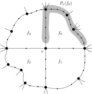
Proof. Let fj be a face of G incident with the vertex v. Traversing the boundary cycle

of fj clockwise from v, let Pv(fj) be the subpath of the boundary cycle starting with the

successor ofv and ending with the predecessor of the last high-degree vertex beforev. (See Figure 2.2 for an illustration.) Let pv(fj) be the number of vertices of Pv(fj). Since each

vertex in NF_{(v) is included in at least one of the paths P}

v(fi) (i= 0, . . . , k−1), we have dF_(v)≤ k−1 X i=0 pv(fi). (2.2)

v Pv(f0) f0 f1 f2 f3

Figure 2.2. The definition of the path Pv(fi) for i = 0 and a vertex v of degree 4.

High-degree vertices are shown as larger dots.

We now boundpv(fi). Assume first thatk ≥3. Recall that every two consecutive

high-degree vertices on the boundary of fi are separated by at most three vertices of degree 2

(Lemma 2.4 (3)). Since exactly two out of the li high-degree vertices are excluded from

Pv(fi), the path Pv(fi) decomposes into li−2 segments, each consisting of at most three

vertices of degree 2 (inG) followed by a high-degree vertex, and one final segment consisting of up to three vertices of degree 2 and no high-degree vertex. The final segment may be empty. We find:

pv(fi)≤4(li−2) + 3 = 4li−5. (2.3)

We also observe an improvement in the following special case. Let us call the path Pv(fi)

deficient if it starts or ends with a high-degree vertex (ofG), or if it contains two consecutive high-degree vertices. In that case, one of the above defined segments contains zero instead of three vertices of degree 2, and we obtain:

pv(fi)≤4li−8 if Pv(fi) is deficient. (2.4)

If k = 2, analogous reasoning yields

pv(fi)≤               

4li−9 ifPv(fi) contains three consecutive high-degree vertices,

4li−7 ifPv(fi) starts with two high-degree vertices,

4li−5 ifPv(fi) ends at a high-degree vertex,

4li−4 ifPv(fi) is deficient,

4li−2 otherwise.

We can now prove part (2) of the lemma. It may be assumed that Pv(f0) starts with a

high-degree vertex, since adjacent 2-vertices have the same face degree. By (2.2) and (2.5),

dF(v)≤pv(f0) +pv(f1)≤(4l0−4) + (4l1 −2) = 4(l0+l1)−6.

Next, we derive part (1). From (2.2) and (2.3), it follows that

dF_(v)≤4 k−1

X

i=0

li−5k. (2.6)

We need to improve this estimate by 3σ, where σ is as defined in the lemma. Let i be such thatli+li+1 ≤25 (indices modulok) and let wbe the first vertex of Pv(fi+1). If the

degree of wis 2, then by part (2) of the lemma,dF_{(w)≤94, contradicting Lemma 2.4 (4).}

Thus, Pv(fi+1) starts with a high-degree vertex and we can apply (2.4) in place of (2.3) to

bound pv(fi+1). This results in an improvement to the upper bound in (2.6) by 3 for each i satisfying li +li+1 ≤ 25, and hence in an improvement by 3σ in total. Part (1) of the

lemma follows.

Let us proceed to part (3). First, note that {l0, l1, l2} 6={2,8,19} by part (1): indeed, we would have

dF_{(v)≤4·(l0+l1+l2)−5·3−3·2 = 95,}

contradicting Lemma 2.4 (4).

Suppose then thatl0 = 3,l1 = 8 andl2 = 19. No vertex of degree 2 inGis incident with bothf0 andf2, since part (2) of the lemma would imply that its face degree is bounded by 4(3 + 19)−6 = 82, contradicting Lemma 2.4 (4). Thus, Pv(f0) starts with a high-degree

vertex, and the same can be proved forPv(f1) by an identical argument.

We claim that no vertex of degree 2 in G is incident with both f1 and f2. Suppose to the contrary that there is such a vertex, and let z be the last 2-vertex encountered on the clockwise boundary cycle of f1 before v. The fact that Pv(f0) starts with a high-degree

vertex implies that Pz(f2) ends at a high-degree vertex. Furthermore, since Pv(f1) starts

with a high-degree vertex, Pz(f1) either starts with two consecutive high-degree vertices

(if z is a neighbor ofv) or contains three consecutive high-degree vertices. By (2.5),

dF(z)≤(4l1−7) + (4l2−5) = 96,

a contradiction with Lemma 2.4 (4). It follows that besides Pv(f0) and Pv(f1), the path

Pv(f2) is also deficient. By (2.4),

dF_{(v)≤4·(l0+l1+l2)−3·8 = 96,}

which again contradicts Lemma 2.4 (4).

We turn to part (4) of the lemma. Unlike the situation in the proof of part (1),NF_{(v, f0)}

is not entirely covered by the sets V(Pv(fi)), where i = 1, . . . , k −1. On the other hand,

only a few vertices ofNF_{(v, f0) are missing in the union of these sets, namely the vertices}

follows Pv(fk−1) on the boundary of fk−1, then the missing vertices are u and the (up to

three) vertices of degree 2 following u. Consequently,

dF(v, f0)≤ k−1 X i=1 pv(fi) + 4, (2.7) and by (2.3), dF(v, f0)≤4 k−1 X i=1 li−5(k−1) + 4 = 4 k−1 X i=1 li−5k+ 9.

Part (5) follows easily from (2.7) using the estimate (2.3) for the face f1 and the estimate (2.4) for f2 (note that l1 +l2 ≤ 25 implies thatPv(f2) is deficient, just as in the

proof of (1)). The proof is thus complete.

2.2

Discharging

Having explored the properties of the graphG, we are ready to use the discharging method to arrive at a contradiction.

We assign an initial charge to the vertices and faces of Gas follows:

• each vertex v receivesd(v)−6 units of charge;

• each face f receives 2|V(f)| −6 units of charge.

The following observation is a well-known consequence of Euler’s formula.

Observation 2.6. The sum of the charges defined above is −12.

In the first phase, we redistribute the charges according to Rules 1–2:

Rule 1. Every face that is not a pseudodigon sends two units of charge to each incident 2-vertex. Each pseudodigon does the same, except that one of the respective 2-vertices receives no charge.

Observe that after the application of Rule 1, the charge of each face is nonnegative. In addition, the charge of every large face is at least 2·20−6 = 34.

Rule 2. Every small face distributes its remaining charge evenly to all incident high-degree vertices (i.e., vertices of degree at least 3). Each large face (i.e., a face of weight at least 20) behaves in the same way, except that it retains a charge of 4.

After applying the above rules the first phase is completed. In the second phase, Rule 3 is applied to the vertices that ended up with negative charge after the first phase.

Rule 3. If a vertex has a negative charge of c and is incident with a large face f, then it receives the charge of −cfrom f.

We will show that the final charge of every vertex and face in G is nonnegative, contra-dicting Observation 2.6.

Recall from Subsection 2.1 that the configuration of a vertex v of G is obtained by ordering the multiset {w(g) :g ∈ F(v)} in a nondecreasing way. If we remove (one copy of) the element w(f) from this ordered multiset, we obtain the f-reduced configuration of

v.

It will be convenient to alter the definition of the weight of a facef and the configuration of a vertex v as follows. The modified weight w′_{(f) of f is defined as 3 if w(f) = 2, and}

w(f) otherwise. Replacing the weight of each face by its modified weight in the definition of the configuration ofv, we obtain themodified configuration ofv. Themodifiedf-reduced configuration of v is obtained from the f-reduced configuration of v in an analogous way.

First we analyze how much charge a vertexvof high degreedreceives by Rule 2. Denote the faces incident with v by fi, i = 0, . . . , d −1, and let ni be the number of 2-vertices

incident withfi. After applying Rule 1, eachfi has charge 2|V(fi)| −6−2ni if fi is not a

pseudodigon, and 2|V(fi)| −6−2(ni−1) otherwise. By Lemma 2.4 (2), fi is not a digon

so in both cases the charge can be written as 2w′_(f

i)−6. Hence, when fi is a small face,

it sends v the charge of

2w′_(f i)−6 w(fi) = 2− 6 w′_(f i) .

(The equality is true as w(fi) = w′(fi) if fi is not a pseudodigon, and 2w′(fi)−6 = 0

otherwise.) On the other hand, when fi is a large face, it sends v

2w′_(f i)−6−4 w(fi) = 2− 10 w′_(f i)

units of charge. Note that in both cases the charge received by v from fi is nonnegative.

In total, the vertex v obtains the nonnegative charge of

X i w′_(fi)<20 2− 6 w′_(f i) + X i w′_(fi)≥20 2− 10 w′_(f i) = 2d−6 X i w′_(fi)<20 1 w′_(f i) −10 X i w′_(fi)≥20 1 w′_(f i) . (2.8)

Next, we establish the following two essential claims. For convenience, we refer to the vertices with a negative charge after the first phase as special vertices. Since the initial charge of a vertex v is d(v)−6 and each vertex receives a nonnegative charge during the application of Rule 2, every special vertex has degree at most 5.

Claim 1. Every special vertex is incident with a large face.

Proof. We proceed by contradiction, assuming that v is a special vertex not incident with any large face. First suppose that d(v) = 2; let f1 and f2 be the two faces incident with

v. As the initial charge of v is −4, at least one of these faces, say f1, is a pseudodigon by Rule 1. By assumption,w(f2)≤19. Hence dF(v)≤78 by Lemma 2.5 (2), a contradiction

to Lemma 2.4 (4).

Therefore, let v be a special vertex of high degree d. Summing its initial charge and the charge (2.8) received by Rule 2 gives

3d−6−6X i 1 w′_(f i) <0, or equivalently, X i 1 w′_(f i) > d 2 −1. (2.9)

We proceed by case analysis; let (l′

i) denote the modified configuration of v. (We write

(l′

i) instead of (li) as a reminder that the configuration is a modified one.) Assume first

that v is of degree 3. Then l′

0 ≤ 5, otherwise (2.9) fails since its left hand side is at most

3·(1/6) which equals its right hand side 1/2. Since v is not incident with any large face, we have l′

1, l′2 ≤19. We aim to use Lemma 2.5 to bound dF(v). Although it is formulated

for ordinary (non-modified) configurations, the monotonicity of the upper bounds ensures that the lemma remains valid if the configuration is a modified one. By Lemma 2.5 (1),

dF_(v)≤4P

il

′

i−21. Consequently, Lemma 2.4 (4) implies that

X

i

l′

i ≥30. (2.10)

If l′

0 = 3 and l′1 ≤ 9, then by (2.10) (li′) is one of the three tuples (3,8,19), (3,9,18),

and (3,9,19). The first of these is excluded by Lemma 2.5 (3), and the remaining two contradict (2.9). If l′

0 = 3 and l′1 >9, then by Lemma 2.3 applied to the tuples (3,10,15)

and (l′

i), in this order, either

P il ′ i ≤28 or P i1/l ′

i ≤1/2. However, that contradicts (2.10)

or (2.9), respectively. Hencel′

0 ≥4. Ifl0′,l′1 = 4, then

P

ili′ ≤27, which is impossible by (2.10). Otherwise we

may use Lemma 2.3 for the tuples (4,5,20) and (l′

i), and obtain a contradiction to (2.10)

or (2.9) again.

Thusd≥4; as we have remarked above,d ≤5. Lemmas 2.5 (1) and 2.4 (4) imply (2.10) again. In particular, (l′

i) cannot be of the form (3,3,3, x). If d = 4, then by Lemma 2.3

applied to the tuple (3,3,4,12), P

il ′ i ≤ 22 or P i1/l ′ i ≤ 1, contradicting (2.10) or (2.9).

Ford= 5, we obtain a similar contradiction by applying Lemma 2.3 to (3,3,3,3,6), which yieldsP il ′ i ≤18 or P i1/l ′ i ≤3/2.

Claim 2. Every large face has a nonnegative final charge.

Proof. Letf be an arbitrary large face ofG. We start by listing the possiblef-reduced or modifiedf-reduced configurations of special vertices incident withf, and for each case we note a lower bound on the charge of these vertices. Take such a special vertex v.

Ifvis a 2-vertex, then by Rule 1 itsf-reduced configuration is (2) and the charge equals

−2.

Now suppose that v is of high degree d. Let (l′

i), i = 1, . . . , d −1, be its modified

f-reduced configuration, and let d′ _{denote the number of large faces incident with v. As} noted earlier, d ≤ 5. By considering the initial charge of v and (2.8), we see that after applying Rule 2,v has charge

3d−6−6 X i w′_(fi)<20 1 w′_(f i) −10 X i w′_(fi)≥20 1 w′_(f i) .

As the charge is negative by assumption, 3d−6−6 X i w′_(fi)<20 1 w′_(f i) −d ′ 2 <0 (2.11)

by the definition of large face. Furthermore, w′_(f

i)≥3 always, and hence

3d−6−2(d−d′_)−d′_/2<0.

Since the left hand side equalsd−6 + 3d′_{/2, we deduce thatd}′ _{= 1 (i.e.,f is the only large} face incident withv), and thatd≤4.

Assume first that d= 3. Then (2.11) reduces to 5 2 −6 1 l′ 1 + 1 l′ 2 <0.

We infer that either l′

1 = 3 and l2′ ≤ 11, or l1′ = 4 and l2′ ≤ 5. The charge of v is at least

1/2−6/l′

2 in the former, and at least 1−6/l′2 in the latter case.

Now let d= 4. By (2.11), 11 2 −6 X i 1 l′ i <0. If some l′

i were greater than or equal to 4, this inequality would not hold. Hence (l′i) =

(3,3,3) and the charge of v is at least −1/2. We summarize the results in Table 1.

Let S denote the set of all special vertices incident with f and R their total charge after the completion of the first phase. We observe the following:

Any two vertices u, v ∈S have at least two common incident faces. (2.12) Suppose the contrary. In view of the possible f-reduced or modified f-reduced configu-rations of u and v listed in Table 1, Lemma 2.5 (4) and (5) implies that both dF_{(u, f)}

and dF_{(v, f) are at most 47. On the other hand, Lemma 2.4 (5) and the assumption}

that f is the only face incident with both u and v imply that dF_{(u, f) +d}F_{(v, f) >95, a}

(modified) f-reduced configuration charge

(2) −2

(3, x),x≤11 ≥1/2−6/x≥ −3/2 (4, x),x≤5 ≥1−6/x≥ −1/2

(3,3,3) ≥ −1/2

Table 1. The proof of Claim 2: the list of possible f-reduced (the first line) or modified f-reduced (the other lines) configurations of special vertices incident with the face f, together with the charge of these vertices.

We proceed to prove Claim 2 by contradiction. Suppose that f has a negative charge after the application of Rule 3. Since the charge of f after the first phase is 4 units (by Rule 2 for large faces), this is equivalent to the condition

R <−4. (2.13)

Considering the lower bounds for charges in Table 1, we see that there are at least three special vertices.

Let v ∈S be a 2-vertex; the other face f′ _{incident with v is a pseudodigon. By Rule 1} and (2.12), every other vertexv′ _{inS is one of the two high-degree vertices v1,v2 incident} with f′_{. Therefore S = {v, v1, v2}; it follows that v1 and v2 are both of degree 3 by} assumption (2.13). This means that F(v1) = F(v2), and hence the configuration of both vertices is the same. Considering (2.13) again, the modified f-reduced configuration of bothv1 and v2 is (3,3).

At this point, we digress by making an auxiliary observation:

Let g be a face of G with w(g) ≤ 3. The intersection of the boundaries of f

and g consists of pairwise disjoint paths, of which at most one is nontrivial; the internal vertices of all these paths are of degree 2 in G. Furthermore, any two vertices of degree 3 incident with both f and g are precisely the end-vertices of such a nontrivial path, and hence, there are at most two such vertices.

(2.14)

To prove this, let us denote the intersection of the boundaries of f and g by H. The assertion about the structure of H is obvious by considering the 2-connectedness of Gand the weights of both f and g. Let P denote the set of the respective paths. Ifv is a vertex of degree 3 incident with f andg, then H must contain an edge incident with v, i.e., v lies on—and hence is an end-vertex of—a nontrivial path in P. The second assertion easily follows.

Applying (2.14) to the face incident with v1 different fromf and f′_{, and recalling that}

f′ _{is a pseudodigon, we infer thatw(f) = 2; a contradiction.}

Thus all vertices in S are of high degree. Suppose that S = {v1, v2, v3}. Then by assumption (2.13), the modified f-reduced configuration of v1, v2, and v3 is (3,3). Hence

by (2.14), no face other than f is incident with the three vertices. By (2.12), G contains three different faces fij, 1 ≤ i < j ≤ 3, incident with both vi and vj and different from

f. By (2.14), the boundary of f is precisely S

P; thus w(f) = 3, a contradiction to the assumption that f is large.

Therefore|S| ≥4. We claim thatGcontains a facef′ _{6=f incident with all the vertices} in S. To prove this, consider three vertices u, x, v in S consecutively encountered on a facial walk off. By (2.12), there is a curve Cuv connecting uand v through a face fuv6=f

of G. Consider any vertex y ∈ S − {u, x, v}. There is a curve Cxy connecting x and y

through a facefxy 6=f. If we letCvu be a curve connectingv touthroughf, thenCuv∪ Cvu

is a closed curve separating x from y. Consequently, Cuv intersects Cxy, and therefore y is

incident with the face fuv. The assertion easily follows.

Now let k := |S|. Then w(f′_{) ≥ k, and consequently the f-reduced configuration of} each v in S contains a number greater than or equal to k. From Table 1, we see that

R≥k 1 2 − 6 k = k 2 −6,

the right side of which is at least −4 by the condition on k. This contradicts assump-tion (2.13).

With the help of the two preceding claims, we can easily finish the proof. By Claim 1 and Rule 3, every special vertex—and hence every vertex—ends up with a nonnegative charge. The final charge of every face is nonnegative as well; Rule 2 and Claim 2 guarantee this for small and large faces respectively. However, as already mentioned, this contradicts Observation 2.6.

3

Lower bound

In this section, we provide examples showing that the best possible constant bound on

χs for the class of 2-connected plane simple graphs is at least 8, and the corresponding

bound for proper spv-colorings is at least 10. Note that for the class of 2-connected plane (multi)graphs, the latter example implies a lower bound of 10 for general spv-colorings. Indeed, if we replace each of its edges by a digon bounding a face, then every spv-coloring of the resulting graph is necessarily a proper spv-coloring of the original simple graph.

First, we focus on the bound for proper spv-colorings. We construct a graph G55 on

ten vertices by linking two disjoint cyclesC1_,C2 _{on five vertices with two additional edges}

whose endvertices in each cycle are adjacent. See Figure 3.1 (a).

By the spv-conditions for the two faces of G55 of length 5, every proper spv-coloring c

must assign each vertex of C1 _{a different color; the same holds for C}2_{. The spv-condition}

for the face of G55 of length 10 then implies that cuses each color precisely once.

Second, we consider the bound on χs (where the coloring is allowed to be improper).

Take a three-sided prism G3 embedded in the plane so that one of its triangular faces is the outer facef3. As observed by Czap and Jendrol’ [3, proof of Lemma 5.1], every coloring

G55 C1 C2 1 2 3 4 5 6 7 8 9 10

(a)The graphG55.

G3 1 2 3 4 5 6 G3 G3 1 2 3 4 5 6 G4

(b) The graphsG3 (left) andG4(right).

G4 G4 G44 1 2 3 4 5 6 7 8 (c) The graphG44.

Figure 3.1. Illustrations for Section 3. The labeled gray areas represent the re-spective subgraphs not depicted in detail. For each graph, the relevant coloring is unique up to symmetry; it is indicated by numerical labels.

c of G3 such that every face of G3 distinct from f3 satisfies the spv-condition colors each boundary vertex of f3 with a different color.

Now construct a graph G4 from a cycle on four vertices by replacing every other edge with a copy ofG3in such a way that the outer facef4ofG4is of length 4; see Figure 3.1 (b). Let c′ _{be a coloring of G}

4 satisfying the spv-condition for each face of G4 other than f4.

When restricted to the vertices of any of the copies ofG3,c′_{has the property of the coloring}

c discussed above. This and the spv-condition for the face of G4 of length 6 imply that c′ assigns a different color to each boundary vertex of f4.

Finally, we reproduce the construction ofG55with copies ofG4 in place of the cycles on five vertices. Thereby we obtain a graphG44 with the outer facef44 of length 8, such that every spv-coloring ofG44 is injective on V(f44). The graph G44 is shown in Figure 3.1 (c).

References

[1] D. P. Bunde, K. Milans, D. B. West, and H. Wu,Parity and strong parity edge-coloring of graphs, Congr. Numer. 187 (2007) 193–213.

[2] D. P. Bunde, K. Milans, D. B. West, and H. Wu, Optimal strong parity edge-coloring of complete graphs, Combinatorica 28 (2008) 625–632.

[3] J. Czap and S. Jendrol’,Colouring vertices of plane graphs under restrictions given by faces, Discuss. Math. Graph Theory 29 (3) (2009) 521–543.

[4] J. Czap, S. Jendrol’, and M. Voigt, Parity vertex colouring of plane graphs, Discrete Math. 311 (6) (2011) 512–520.

[5] J. Czap, S. Jendrol’, F. Kardoˇs and R. Sot´ak, Facial parity edge colouring of plane pseudographs, Discrete Math. 312 (17) (2012) 2735–2740.