Copyright and use of this thesis
This thesis must be used in accordance with the
provisions of the Copyright Act 1968.
Reproduction of material protected by copyright
may be an infringement of copyright and
copyright owners may be entitled to take
legal action against persons who infringe their
copyright.
Section 51 (2) of the Copyright Act permits
an authorized officer of a university library or
archives to provide a copy (by communication
or otherwise) of an unpublished thesis kept in
the library or archives, to a person who satisfies
the authorized officer that he or she requires
the reproduction for the purposes of research
or study.
The Copyright Act grants the creator of a work
a number of moral rights, specifically the right of
attribution, the right against false attribution and
the right of integrity.
You may infringe the author’s moral rights if you:
- fail to acknowledge the author of this thesis if
you quote sections from the work
- attribute this thesis to another author
- subject this thesis to derogatory treatment
which may prejudice the author’s reputation
For further information contact the University’s
Director of Copyright Services
S TAT I S T I C A L M E T H O D S F O R T H E A N A LY S I S A N D I N T E R P R E TAT I O N O F R N A - S E Q D ATA
e l l i s pat r i c k
A thesis submitted in fulfilment of the requirements for the degree of
Doctor of Philosophy
School of Mathematics and Statistics The University of Sydney
Ellis Patrick :Statistical methods for the analysis and interpretation of RNA-Seq data,Doctor
A B S T R A C T
In the post-genomic era, sequencing technologies have become a vital tool in the global analysis of biological systems. RNA-Seq, the sequencing of messenger RNA, in partic-ular has the potential to answer many diverse and interesting questions about the inner workings of cells. Despite the decreasing cost of sequencing data, the majority of RNA-Seq experiments are still suffering from low replication numbers. The statist-ical methodology for dealing with low replicate RNA-Seq experiments is still in its infancy and has room for further development. Incorporating additional information from publicly accessible databases may provide a plausible avenue to overcome the shortcomings of low replication. Not only could this additional information improve on the ability to find statistically significant signal but this signal should also be more biologically interpretable.
This thesis is separated into three distinct statistical problems that arise when pro-cessing and analysing RNA-Seq data. Firstly, the use of experimental data to customise gene annotations is proposed. When customised annotations are used to summarise read counts, the corresponding measures of transcript abundance include more inform-ation than alternate summarisinform-ation approaches and offer improved concordance with qRT-PCR data. A moderation methodology that exploits external estimates of variation is then developed to address the issue of small sample differential expression analysis. This approach performs favourably against existing approaches when comparing gene rankings and sensitivity. With the aim of identifying groups of miRNA-mRNA regu-latory relationships, a framework for integrating various databases of prior knowledge with small sample miRNA-Seq and mRNA-Seq data is then outlined. This framework appears to identify more signal than simpler approaches and also provides highly in-terpretable models of mRNA regulation. To conclude, a small sample miRNA-Seq and mRNA-miRNA-Seq experiment is presented that seeks to discover miRNA-mRNA
regulatory relationships associated with loss of Notch2function and its links to
neuro-degeneration. This experiment is used to illustrate the methodologies developed in this thesis.
P U B L I C AT I O N S A N D P R E S E N TAT I O N S
Some of the methods, concepts, analyses and results in this thesis have appeared pre-viously in the following:
p u b l i c at i o n s
Ellis Patrick, Michael Buckley, David Ming Lin, and Yee Hwa Yang. Improved mod-eration for gene-wise variance estimation in RNA-Seq via the exploitation of external
information. BMC Genomics,14 Suppl1:S9,2013.
Ellis Patrick, Michael Buckley, and Yee Hwa Yang. Estimation of data-specific
con-stitutive exons with RNA-Seq data. BMC Bioinformatics,14:31,2013.
Pengyi Yang, Ellis Patrick, Shi-Xiong Tan, Daniel Fazakerley, James Burchfield, Chris-topher Gribben, Matthew Prior, David James and Yee Hwa Yang. Direction pathway analysis of large-scale proteomics data reveals novel features of the insulin action path-way. Accepted in Bioinformatics,2013.
p r e s e n tat i o n s
Optimising a genomic annotation for the analysis of RNA-Seq data. Australasian
Mi-croarray and Associated Technologies Association (AMATA),2010, Hobart, TAS.
Improved moderation for gene-wise variance estimation in RNA-Seq. Australian
Stat-istical Conference (ASC),2012, Adelaide, SA.
Improved moderation for gene-wise variance estimation in RNA-Seq.Asia Pacific
Bioin-formatics Conference (APBC),2013, Vancouver, BC.
An integrative analysis of miRNA-Seq and mRNA-Seq data. Western North American
Region of the International Biometrics Society (WNAR),2013, Los Angeles, CA.
An integrative analysis of miRNA-Seq and mRNA-Seq data. The57th Annual Meeting
of the Australian Mathematical Society (AustMS),2013, Sydney, NSW.
“A bird doesn’t sing because it has an answer, it sings because it has a song." - Maya Angelou
A C K N O W L E D G M E N T S
Through the course of my studies I have been incredibly fortunate to have been sur-rounded by so many amazing personalities. While I could not possibly list them all, these amazing people have shaped my understanding of statistics, biology and life in general.
I would like to start by thanking my supervisor Jean for everything she has done for me. She has been an inspiration, incredibly patient and always made me feel like my opinions have value. I would not be where I am now, for so many reasons, without her. I am so glad that she took me on five years ago and could never effectively express my appreciatation for sharing all her experience, ideas and time.
I would like to also thank all of the following: My associate supervisor Mike for being a constant source of knowledge, reassurance and encouragement. Dave Lin for being such an awesome bloke, always having time for me and having such an articulate knowledge of biology. Also, the rest of his lab for making me feel so welcome. Anna Campain for all our conversations and making me feel very much like the younger sibling. Garth Tarr for simply putting up with me, he’s made the past four years so much easier. Neville Weber for not only sparking my interest in statistics but always finding time to offer me guidance and advice. John Ormerod for becoming both a friend and mentor. Samuel Mueller for always leaving his door open. Everyone that
has participated in Monday lab meetings and all the faculty on the8th floor for any
advice, wisdom or laughs they have shared with me. Pengyi for coping with my blunt-ness. David James for appreciating my sense of humour. Terry Speed for his valuable opinions and advice. Jennifer Chan and Ross Sparks for giving me a chance to cut my teeth.
Of course I could never have made it through my studies without the emotional and financial support of my family. I have never felt any pressure to be anything other than myself or do anything other than those things I’d like to do. I’d also like to thank my fiance Tanya for falling in love with this poor student and for all her patience and support.
C O N T E N T S
1 Introduction 1
1.1 Background . . . 2
1.1.1 The biology of a cell . . . 2
1.1.2 Technologies for measuring gene expression . . . 4
1.1.3 Common biological questions . . . 6
1.1.4 A common RNA-Seq pipeline . . . 6
1.2 Motivational data . . . 9
1.3 Outline of the thesis . . . 10
2 Summarisation – The estimation of data-specific constitutive exons with RNA-Seq data 11 2.1 Genes, alternative splicing and isoforms . . . 12
2.2 Summarisation of read counts . . . 15
2.2.1 Estimation of constitutive exons . . . 16
2.2.2 Processing exon annotation . . . 18
2.3 exClust - Estimate data-specific constitutive exons through clustering . . 20
2.4 Evaluation study . . . 23
2.4.1 Data . . . 23
2.4.2 Evaluation criterion and results . . . 25
2.5 Conclusions and further discussion . . . 32
3 Differential expression – Improved moderation for gene-wise variance estim-ation in RNA-Seq via the exploitestim-ation of external informestim-ation 34 3.1 Modelling RNA-Seq data . . . 35
3.2 Tshrink+ . . . 39
3.3 Evaluation study . . . 40
3.3.1 Data . . . 41
3.3.2 Evaluation strategies and results . . . 42
3.4 Conclusions and further discussion . . . 50
4 Functional, network & pathway analysis – Using pathway information to help integrate small sample miRNA-Seq and mRNA-Seq data 52 4.1 miRNA . . . 53
4.2 Combining p-values . . . 55
4.2.1 Simulation . . . 56
4.3 pMiM - Pathway, microRNA and mRNA integration . . . 60
4.4 Evaluation Study . . . 65
4.4.1 Data . . . 65
4.4.2 Evaluation strategies and results . . . 66
4.5 Conclusions and further discussion . . . 71
5 Case study of the Lin data 73 5.1 Design . . . 74 5.2 Mapping . . . 75 5.3 Summarisation . . . 77 5.4 Normalisation . . . 80 5.5 Differential expression . . . 82 vi
c o n t e n t s vii
5.6 Functional, network & pathway analysis . . . 87
5.6.1 Pathway analysis . . . 87
5.6.2 Integration of miRNA and mRNA data . . . 88
5.7 Conclusions and further discussion . . . 89
6 Conclusion 91 a Additional information for Chapter2 95 a.1 Detection of differential alternative splicing . . . 96
a.2 Additional figures and tables . . . 96
b Additional information for Chapter3 98 b.1 Normalisation for Bottomly dataset . . . 99
b.1.1 GC content . . . 99
b.1.2 Other Technical effects . . . 99
b.2 Additional Figures . . . 100
c Additional information for Chapter4 103 c.1 Additional Figures . . . 104
L I S T O F F I G U R E S
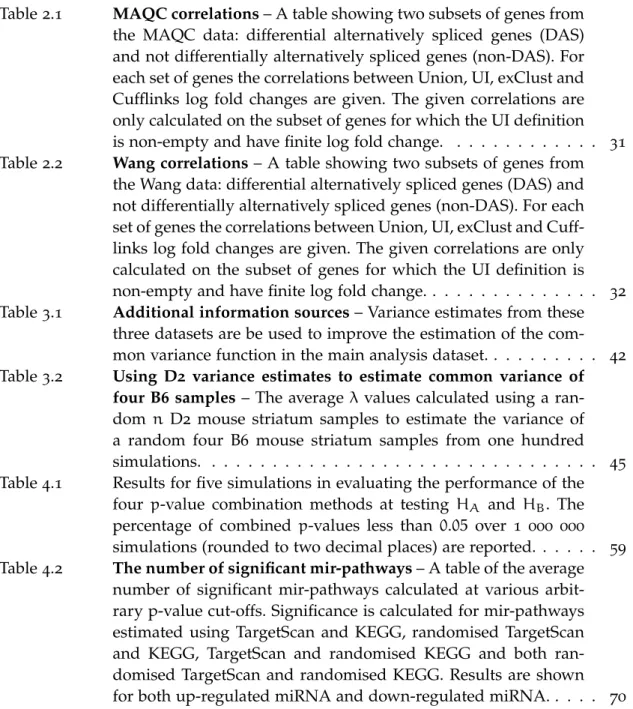
Figure1.1 The Central Dogma of Molecular Biology – An illustration of
the Central Dogma of Molecular Biology, a simplified concep-tualisation of the flow of genetic information within the cell. In-formation stored in DNA can be transcribed into messenger RNA which can then move outside of the nucleus and be translated
into a functional protein. . . 3
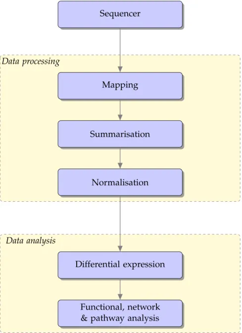
Figure1.2 RNA-Seq analysis pipeline – A flow chart describing a typical
RNA-Seq analysis pipeline. This pipeline consists of two broad steps, data processing and data analysis. Data processing includes aligning reads to a genome (mapping), summarising how many of these reads lie in particular regions of the genome (summarisa-tion) and correcting for any systematic technical variation (nor-malisation). Data analysis consists of identifying genes that have changed in expression between two conditions (differential ex-pression) and some higher level analysis to improve the
inter-pretability of the results (functional, network & pathway analysis). 7
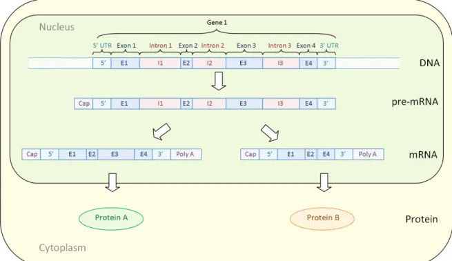
Figure2.1 Transcription and alternative splicing – A toy example
demon-strating how the information stored in one gene can be tran-scribed, spliced and translated to form multiple distinct proteins.
Gene 1, contains four exons, three introns and a 5’ and 3’ UTR.
This information can be transcribed to form a pre-mRNA that has
had a cap added to its5’ end. The introns in the pre-mRNA are
spliced out to form a mature mRNA. This pre-mRNA can be al-ternatively spliced to form a mature mRNA that contains all four exons and a mature mRNA that has had its third exon removed. These two mature mRNA can then move outside of the nucleus of the cell into the cytoplasm to be translated into Protein A and
Protein B. . . 13
Figure2.2 Effect of differential alternative splicing on gene counts– A toy
example of a gene with two isoforms is considered. The number of reads that aligned to each exon of the gene are provided for three biological samples. The sums of these exon counts are also
included for each sample. . . 17
List of Figures ix
Figure2.3 Processing exon annotation– A graphic describing how the
notation of two overlapping genes is processed into an exon an-notation appropriate for the use of exClust. The isoform annota-tion can be used to define a set of disjoint exon regions that could be rejoined to describe any of the known isoforms of the gene. It is these disjoint exon regions that are used as the exon annota-tion in exClust. Exon regions which overlap multiple genes are ignored. The set of UI exons are also shown for these two genes and are simply the exons that are present in all the annotated
isoforms. . . 19
Figure2.4 Identifying constitutive exons – Plot of exons selected by
ex-Clust for a particular gene. A clustering dendrogram of the exons is formed by apply Ward’s linkage hierarchical clustering to the
distance matrix1−ΣEg. Cutting the dendrogram at the dashed red
line results in the creation of three subgroups of exons (each box here contains a subgroup). For each subgroup the average cover-age of the two exons in that subgroup with the highest covercover-age is calculated. The subgroup with the highest average coverage (the shaded subgroup) is selected to represent the DSC exons for
this gene. . . 22
Figure2.5 Concordance Plot– Concordance plot with the RNA-Seq log fold
changes on the y-axis and qRT-PCR log fold changes on the x-axis. For the RNA-Seq data we use the union of all exons within a gene to summarise our counts where a value of one is added to the count of every gene. The black circles are those genes for which the UI definition is non-empty. The blue triangles are the
386genes for which the UI definition is empty. The red dots are
those genes that our method identified as having a change in
isoforms and had a non-empty UI definition. . . 28
Figure2.6 Residual Plot – After fitting a straight line through the plot in
Figure 2.5, this figure plots on the y-axis the residuals for the
genes identified as having a change in isoforms for three different annotations, union of all exons (black dots), UI definition (blue triangles) and exClust (red circles), and cufflinks (purple cross)
ordered by qRT-PCR fold change. . . 29
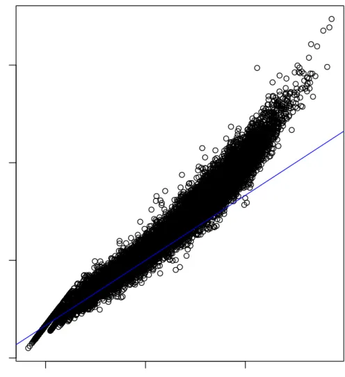
Figure3.1 The mean-variance relationship in RNA-Seq data on a log-log
scale – This figure demonstrates the stong mean-variance
rela-tionship observed in RNA-Seq data. For each gene from the ten
Bottomly B6samples described in Section3.3the mean and
vari-ance are calculated. These means and varivari-ances are then plotted against each other on a log-log scale. The blue line corresponds
List of Figures x
Figure3.2 Effect of utilising different sources of information on the
es-timation of λ – Variance estimates from the external datasets
(Table3.1) and gene length are used to aid in the estimation of the
common variance functions of one hundred comparisons ofnB6
and nD2 mouse striatum samples. The average λ value is
plot-ted for eachncomparison and information source fornranging
from two to five. The parameterλis the ratio of the expected and
average squared error of the gene sample variance to the com-mon variance. The information source “None” corresponds to us-ing no extra information, “Striatum” the RNA-Seq samples from
Polymenidou et al (2011) and “Striatum Microaray” the
microar-ray striatum samples from Bottomly et al (2011). The information
sources have been sorted by theirλvalues fornequals two. . . 44
Figure3.3 Comparing six DE methods on a4 vs4comparison– One
hun-dred random comparisons of four B6and four D2mouse striatum
samples for six DE methods. Average TP and FP are calculated for the full range of p-value cut-offs. The TPR and FPR are plot-ted against each other in a) to form ROC curves and displayed
in the region for FPR less than 0.01 as this is most relevant for
calling DE. For any given FPR a method with a larger TPR is deemed to have ranked the genes better. In b) the number of TP (in bold) and FP are plotted for a range of p-value cut-offs. The x-axis is in log-scale. The grey dashed vertical line corresponds
to a Bonferroni adjusted cut-off of0.05. . . 47
Figure3.4 Partial AUCs for a range ofnvsncomparisons– One hundred
random comparisons ofnB6andnD2mouse striatum samples a
performed for six DE methods fornranging from two to five. For
each method and n, partial areas under the ROC curves (partial
AUC) are calculated for the regions of FPR less than0.01 . . . 48
Figure3.5 The number of True and False Positives for a range of nvs n
comparisons– One hundred random comparisons ofnB6andn
D2mouse striatum samples a performed for six DE methods for
n ranging from two to five. For each method and n, the
conser-vative Bonferroni adjusted cut-off of0.05 is used to calculate the
average number of (a) True Positives and (b) False Positive are
counted. . . 49
Figure4.1 p-value cut-offs for various combination methods – A plot
il-lustrating a p-value cut-off of 0.05 for various p-value
combina-tion methods in a two dimensional setting. The p-value cut-off is plotted in the negative z-score space so that a small p-value cor-responds to a large positive z-score. The combination methods under consideration are Fisher (red), Stouffer (blue), maxP (pink)
List of Figures xi
Figure4.2 Data matrices and summary statistics – A visual representation
of the input data matrices which include the matched mRNA-and miRNA-Seq data, a pathway database mRNA-and the miRNA tar-get binding predictions. Also represented are the corresponding summary statistics used which are the statistics from a moder-ated two-sample t-test performed on the mRNA-Seq data, the statistics from a moderated two-sample t-test performed on the miRNA-Seq data and the cross correlations or probability of ob-serving the cross correlations between the miRNA- and
mRNA-Seq data. . . 61
Figure4.3 Number of mir-pathways that containngenes before and after
randomisation – For n = 1, ...,20 the average number of
mir-pathways that contain n genes are plotted on a log-scale. These
are plotted for mir-pathways calculated using TargetScan and KEGG, randomised TargetScan and KEGG, TargetScan and ran-domised KEGG and both ranran-domised TargetScan and
random-ised KEGG. . . 68
Figure4.4 Number of mir-pathways that contain 3, 4 or 5 genes before
and after randomisation– For n= 3, 4and 5the average
num-ber of mir-pathways that contain ngenes are plotted. These are
plotted for mir-pathways calculated using TargetScan and KEGG, randomised TargetScan and KEGG, TargetScan and randomised
KEGG and both randomised TargetScan and randomised KEGG. . 69
Figure4.5 TP vs FP from PubMed search– True Positives (TP) are plotted
against False Positives (FP) for the small FPR region of Figure
C.1. The plotted lines are for four methods, miRNA DE (black),
cMimDE (blue), pMimDE (green) and pMimCor (red). . . 71
Figure5.1 Number of mapped mRNA– (a) A histogram of the number of
reads that were sequenced for each mRNA sample. (b) A bar plot of the percentage of these reads that mapped uniquely, failed to
map and mapped to multiple regions on the genome. . . 76
Figure5.2 Number of base pairs cut by cutAdapt– A histogram describing
the number of reads that had a certain number of base pairs cut
by cutAdapt. . . 78
Figure5.3 Number of mapped miRNA – (a) A histogram of the number
of reads that were sequenced for each miRNA sample. (b) A bar plot of the percentage of these reads that mapped uniquely, failed
to map and mapped to multiple regions on the genome. . . 79
Figure5.4 Plot of summarised miRNA counts vs mRNA counts – Gene
counts from the mRNA and miRNA enriched samples are plot-ted against each other on a log-log scale. The hollow circles are
Figure5.5 MA-plot illustrating TMM normalisation – An MA-plot
gener-ated for one of the WT mRNA samples. The y-axis is the log ratio of one of the WT samples and the average across all samples (M) and the x-axis are the average gene counts across all samples (A).
The solid blue line is M= 0 and the dashed red line is the line
fitted by TMM. . . 83
Figure5.6 P-value histograms for four different methods – P-value
his-tograms were generated from the comparison of WT and NCN mice using a two sample t-test (T), a two sample t-test using a fitted common variance (Tcommon), a moderated t-test (Tshrink) and a moderated t-test using variance information from the Borchelt
mice (Tshrink+). . . 86
Figure A.1 Verification of the Poisson assumption for the MAQC and Wang
data– The squared standardised residuals are plotted against the
average for each gene in the a) MAQC and b) Wang datasets. The
blue line is they=xline. The red circles correspond to the fitted
points found using local smoothing. . . 97
Figure A.2 Gene exon counts– For two genes, a) ENSG00000103769and b)
ENSG00000076662, the exon counts for each sample are plotted.
The first seven samples are brain and the second seven are UHR. A line is drawn between the points to make the behaviour of each exon easier to follow. Highlighted in red are the UI exons
and dashed blue are the exClust exons. . . 97
Figure B.1 ROC of normalised data using arrays as truth – Average TPR
and FPR are calculated from 100 random four B6 vs four D2
mouse striatum comparisons for four normalisation methods us-ing results from an a) Affymetrix and b) Illumina array as truth. These are plotted against each other to form ROC curves. For any given FPR a method with a larger TPR is deemed to have ranked
the genes better. . . 100
Figure B.2 Boxplots of log variances –Boxplots of the log variance of the
within sample gene ranks for four normalisation methods. All normalisation methods on average reduce the variance of the
ranking of the genes. . . 101
Figure B.3 Residual plots for the MAQC and Wang data– Average TPR and
FPR are calculated from a)100random four B6vs four D2mouse
striatum comparisons and b) 100random five vs five D2 mouse
striatum comparisons for six DE methods. These are calculated using results from an Affymetrix array experiment as truth. The TPR and FPR are plotted against each other to form ROC curves
and displayed in the region for FPR less than 0.1 as this is most
relevant for calling DE. For any given FPR a method with a lar-ger TPR is deemed to have ranked the genes better. T and Tshrink both improve in performance relative to edgeR and DESeq when moving from the four vs four comparison to the five vs five
com-parison. . . 102
List of Tables xiii
Figure C.1 ROC plot from PubMed search – ROC curves are plotted for
various methods as decribed inLiterature search strategy. The search
term used is neurodegeneration. True Positive Rates (TPR) are plotted against False Positive Rates (FPR) for four methods, miRNA
DE (black), cMimDE (blue), pMimDE (green) and pMimCor (red). 104
L I S T O F TA B L E S
Table2.1 MAQC correlations– A table showing two subsets of genes from
the MAQC data: differential alternatively spliced genes (DAS) and not differentially alternatively spliced genes (non-DAS). For each set of genes the correlations between Union, UI, exClust and Cufflinks log fold changes are given. The given correlations are only calculated on the subset of genes for which the UI definition
is non-empty and have finite log fold change. . . 31
Table2.2 Wang correlations– A table showing two subsets of genes from
the Wang data: differential alternatively spliced genes (DAS) and not differentially alternatively spliced genes (non-DAS). For each set of genes the correlations between Union, UI, exClust and Cuff-links log fold changes are given. The given correlations are only calculated on the subset of genes for which the UI definition is
non-empty and have finite log fold change. . . 32
Table3.1 Additional information sources– Variance estimates from these
three datasets are be used to improve the estimation of the
com-mon variance function in the main analysis dataset. . . 42
Table3.2 Using D2 variance estimates to estimate common variance of
four B6 samples– The averageλ values calculated using a
ran-dom n D2 mouse striatum samples to estimate the variance of
a random four B6 mouse striatum samples from one hundred
simulations. . . 45
Table4.1 Results for five simulations in evaluating the performance of the
four p-value combination methods at testing HA and HB. The
percentage of combined p-values less than 0.05 over 1 000 000
simulations (rounded to two decimal places) are reported. . . 59
Table4.2 The number of significant mir-pathways– A table of the average
number of significant mir-pathways calculated at various arbit-rary p-value cut-offs. Significance is calculated for mir-pathways estimated using TargetScan and KEGG, randomised TargetScan and KEGG, TargetScan and randomised KEGG and both ran-domised TargetScan and ranran-domised KEGG. Results are shown
List of Tables xiv
Table5.1 Design of the experiment – This table describes the design of
the experiment performed by the Lin lab. Listed are the genotype, age and sex of the mice as well as whether they were treated with BSO. Also included is the lane of the flowcell that each sample
was sequenced on. . . 75
Table5.2 Number of reads summarised – Tabulated are the number of
reads summarised by the Union, UI and exClust approaches. For each approach the number of genes with average counts greater
than zero and twenty are also included. . . 79
Table5.3 Table of results from mRNA DE – The number of DE genes
are reported from the comparison of WT and NCN mice by four
DE methods for an arbitrary 0.05 p-value cut-off; a two sample
t-test (T), a two sample t-test using a fitted common variance (Tcommon), a moderated t-test (Tshrink) and a moderated t-test using variance information from the Borchelt mice (Tshrink+). The number of DE genes are also reported after adjusting for multiple testing using the Benjamini-Hochberg and Bonferroni
methods. . . 84
Table5.4 Table of results from miRNA DE – The number of DE miRNA
are reported from the comparison of WT and NCN mice by four
DE methods for an arbitrary 0.05 p-value cut-off; a two sample
t-test (T), a two sample t-test using a fitted common variance (Tcommon), a moderated t-test (Tshrink) and a moderated t-test using variance information from the Borchelt mice (Tshrink+). The number of DE miRNA are also reported after adjusting for multiple testing using the Benjamini-Hochberg and Bonferroni
methods. . . 85
Table5.5 Table of results GOSeq – GOseq was used to perform a
path-way over-representation test on the list DE genes from Tshrink+.
Listed are the pathways that had a p-value less than0.05. . . 87
Table5.6 Table of results from pMimCor for over expressed miRNA. –
Listed are the top ten mir-pathways found using pMimCor whose miRNA were over expressed in the NCN samples. The corres-ponding miRNA and KEGG pathway are listed, as well as, the p-value from pMimCor, the miRNA Tshrink+ p-value and the
number of genes in the mir-pathway. . . 89
Table5.7 Table of results from pMimCor for under expressed miRNA.–
Listed are the top ten mir-pathways found using pMimCor whose miRNA were under expressed in the NCN samples. The corres-ponding miRNA and Kegg pathway are listed, as well as, the p-value from pMimCor, the miRNA Tshrink+ p-value and the
number of genes in the mir-pathway. . . 90
Table A.1 Log fold changes for different summarisation methods – For
two genes, ENSG00000103769 and ENSG00000076662, log fold
changes are reported for four summarisation methods and
A B B R E V I AT I O N S
3’ UTR Three prime untranslated region
5’ UTR Five prime untranslated region
bp Basepair
BSO Pro-oxidant buthionine sulphoximine
C6 C57BL/6J mouse strain
D2 DBA/2J mouse strain
DAS Differentially alternatively spliced
DNA Deoxyribonucleic acid
DE Differentially expressed
DSC Data-specific constitutive
FDR False discovery rate
FP False positives
FPKM The number of fragments per kilobase of exon per million fragments
that were mapped
FPR False positive rate
mRNA Messenger-RNA
mRNA-Seq Sequencing of mRNA molecules
miRNA Micro-RNA
miRNA-Seq Sequencing of miRNA molecules
NCN Nestin-cre/N2flox
qRT-PCR Quantitative real time polymerase chain reaction
RNA Ribonucleic acid
RNA-Seq Sequencing of RNA molecules
ROC Receiver operating characteristic
pAUC Partial area under the receiver operator curve
TMM Trimmed means of M-values
TP True positives
TPR True positive rate
WT Wild type
1
I N T R O D U C T I O N
1.1 b a c k g r o u n d 2
1.1 b a c k g r o u n d
Since the announcement in May2007of the sequencing of James Watson’s entire
gen-ome using454Life Sciences, next-generation sequencing technologies made headlines
around the world, demonstrating the advancement in genome sequencing. These
tech-nologies saw the beginning of projects such as the $1000 genome project, the 1000
genome project and the ENCODE project, all of whose completion was expected to make huge impacts on the understanding of human health. These projects have high-lighted how complex the biology of a cell and all its regulatory mechanisms are. While these new technologies have ushered in a torrent of new biological knowledge, they have also underlined that we have a lot more knowledge to acquire.
Next-generation (or second-generation) high-throughput sequencing produces data-sets that are incredibly exciting for statisticians. While these technologies can be used to answer a vast array of biological questions, many of the datasets that are produced
lie squarely in the domain of very smalln, extremely largep. That is, it is not unusual
to see datasets with three or fewer biological replicates in each condition making meas-urements on tens of thousands of genes. This framework flies in the face of classical statistics and provides an exciting new world for statisticians to explore.
1.1.1 The biology of a cell
Over the past ten years, the scientific community has begun to appreciate how complex the biological system within a cell really is. Just as the community is on the verge of cracking a problem that is thought to provide a significant leap in understanding and treatment of human health, another level of complexity in the cell is discovered. Epigenetics was one such paradigm shift. Biological mechanisms such as alternate splicing, methylation, histone modification and non-coding RNA, have all provided insights into the complexity of the cell and its regulation. It has become apparent that we are not just a product of our DNA.
1.1 b a c k g r o u n d 3
Figure1.1:The Central Dogma of Molecular Biology– An illustration of the Central
Dogma of Molecular Biology, a simplified conceptualisation of the flow of genetic information within the cell. Information stored in DNA can be tran-scribed into messenger RNA which can then move outside of the nucleus and be translated into a functional protein.
When first learning about cell biology it is often useful to consider a simplified flow
of information (Figure 1.1). The Central Dogma of Molecular Biology (Crick, 1970)
states that in the nucleus of your cells, information contained on your DNA (often called genes) can be transcribed into messenger RNA which can move outside of the nucleus and be translated into a functional protein. This flow of information is gener-ally referred to as gene expression. How it is regulated, inhibited and can be manipu-lated is of great interest to the scientific community.
Deoxyribonucleic acid (DNA) is located in the nucleus of the cell and consists of two complementary strands of sequences of nucleotides that are arranged in a double helix. A strand of DNA consists of a three billion long sequence of the four nucleotides aden-ine (A), thymaden-ine (T), cytosaden-ine (C) and guanaden-ine (G). The two strands are complementary in the sense that if you have an adenine in a position on one strand then you know that there is a thymine in the same position on the other strand. Likewise if there is a cytosine in a position on one strand then there is a guanine in the same position on the other strand. While the DNA within a cell has a very complex structure, it is generally annotated as a single linear sequence of base-pairs (A-T, T-A, C-G, G-C) which is split
up into chromosomes (23for humans).
Around 1–2% of human DNA contains information, or blueprints, for building
proteins. These regions are generally referred to as genes. Transcription is a process that copies the information of a gene into a complementary single stranded
Ribo-1.1 b a c k g r o u n d 4
nucleic acid (RNA) molecule, messenger RNA (mRNA). RNA again consists of four nucleotides adenine (A), uracil (U), cytosine (C) and guanine (G) with uracil repla-cing its DNA counterpart thymine. After being transcribed, mRNA undergoes post-transcriptional modifications and then moves outside of the nucleus into the cytoplasm of the cell to be translated into a protein. Some of these post-transcriptional modifica-tions are referred to as alternative splicing and allow the information of a gene to be arranged in many different ways (isoforms), such that the information stored in one gene could be translated to make many different proteins.
1.1.2 Technologies for measuring gene expression
There are many ways to measure gene expression. This thesis contains gene expres-sion data generated with qRT-PCR, microarrays and next generation high-throughput sequencing. These approaches are outlined in the following.
1.1.2.1 qRT-PCR
Quantitative real time polymerase chain reaction (qRT-PCR) is often seen as a gold standard for measuring gene expression and will often be used to validate a small set
of genes. The effectiveness of qRT-PCR relies on the design of a12–500basepair probe
that is complementary and specific to a portion of the mRNA of interest. A fluorescent dye can be attached to these probes making it possible to quantify how many of them bind to sequence of interest in the sample. QRT-PCR is a cyclic process of iteratively doubling the amount of product in the sample via PCR while measuring the fluores-cence emitted by the labelled probes. By tracking this fluoresfluores-cence and comparing the rate that it doubles to a control gene, the relative quantity of a mRNA of interest can be measured.
1.1.2.2 Microarrays
Microarrays facilitated the high-throughput measurement of gene expression making it possible to measure the expression of tens of thousands of genes simultaneously. They achieved this by arranging thousands of probes spatially on a slide, either printed
1.1 b a c k g r o u n d 5
on directly in spots or coded onto beads. After amplification, fluorescent labels are attached to the mRNA samples which are then washed across the slides and treated so that the mRNA will hybridise (or bind to) any complementary probes on the array. Relative quantities of mRNA can then be determined by exciting the fluorescent labels with a laser and observing the intensity of light from different spots on the array.
One of the key disadvantages of microarrays is their reliance on probes. These probes have to be known in advance and generally selected in such a way so as to cover as much of an organisms transcriptome as possible. Some probes may also suffer from cross-hybridisation, that is, mRNA binding to probes that were not specifically de-signed to detect them.
1.1.2.3 High-throughput sequencing
Next generation high-throughput sequencing breaks the reliance on having to design probes for an experiment. While high-throughput sequencing platforms differ in their chemistry and protocols, their processed outputs are generally similar. The sequencing
platforms take a sample of fragmented RNA as input and then read off 25–400base
pair regions at the ends of these fragments. The output of these sequenced regions,
sequences of base pairs, are referred to as reads. These reads are used to infer the
presence and quantity of RNA in the sample.
The development of high-throughput sequencing technologies has made it possible to sequence the transcriptome at a much higher resolution and coverage than was previously available. Sequencing of mRNA samples (RNA-Seq) has a dynamic range
larger than that of microarrays (Wanget al.,2009). This, combined with its high level of
reproducibility (Mortazaviet al.,2008) and falling cost, makes high-throughput
sequen-cing technologies an increasingly attractive alternative to microarrays for transcriptome
analysis. The three most prominent sequencing platforms are 454 Life Sciences,
1.1 b a c k g r o u n d 6
1.1.3 Common biological questions
There are many uses for high-throughput sequencing, with the technology being used to address various biological problems. These problems can be broken up into two main categories:
1. reassembling what we measured to find out what was present (de novo assembly,
SNP identification, motif finding) and
2. quantifying and comparing how much of a product was present (differential
expression, tissue profiling).
High-throughput sequencing can also be used to sequence various preselected subsets of RNA and/or DNA to sequence. These include:
DNA-Seq — genome sequencing,
RNA-Seq — transcriptome sequencing,
miRNA-Seq — microRNA sequencing and
ChIP-Seq — chromatin immunoprecipitation sequencing.
All of these various biological problems and applications have their own technical intricacies which have themselves generated many interesting and challenging compu-tational and statistical problems. In this thesis we will consider some of the analytical problems that arise when detecting differentially expressed genes with RNA-Seq data.
1.1.4 A common RNA-Seq pipeline
Many RNA-Seq experiments are generated with the common biological goal of identi-fying differentially expressed genes or transcripts – that is, to determine if the tran-scription of any genes is different between any two phenotypically distinct cellular populations. A typical RNA-Seq data analysis workflow with this focus consists of
many steps (Oshlacket al.,2010); these steps generally consist of mapping,
summarisa-tion, normalisasummarisa-tion, differential expression and systems biology (functional, network &
1.1 b a c k g r o u n d 7
and summarisation asdata processing steps and differential expression and functional,
network & pathway analysis asdata analysissteps.
Data processing
Data analysis
Sequencer
Mapping
Summarisation
Normalisation
Differential expression
Functional, network
& pathway analysis
Figure1.2:RNA-Seq analysis pipeline – A flow chart describing a typical RNA-Seq
analysis pipeline. This pipeline consists of two broad steps, data processing and data analysis. Data processing includes aligning reads to a genome (mapping), summarising how many of these reads lie in particular regions of the genome (summarisation) and correcting for any systematic technical variation (normalisation). Data analysis consists of identifying genes that have changed in expression between two conditions (differential expression) and some higher level analysis to improve the interpretability of the results (functional, network & pathway analysis).
1.1 b a c k g r o u n d 8
Mapping is the process of aligning reads to a reference genome (or transcriptome) and inferring from where they may have been transcribed. Most sequencing techno-logies are limited in the length of the read they can sequence and hence sequence limited intervals of fragmented transcripts. Mapping millions, billions or trillions of reads back to reference genomes that have billions of base pairs is both
computation-ally and statisticcomputation-ally intensive (Langmeadet al., 2009). The process of identifying and
aligning various splice variants only further adds to this bioinformatics burden (Bona
et al.,2008; Trapnellet al.,2009; Bryantet al.,2010; Wanget al.,2010b).
Summarisation is the process of simplifying the mapping information into read counts (or expression values) for all genes (or isoforms) of interest. While identify-ing the presence of an isoform is difficult, as many of these transcript fragments are present in multiple isoforms, it is also a statistically challenging problem to quantify
expression of these isoforms (Jiang and Wong,2009; Liet al.,2010; Trapnellet al.,2010).
To avoid inferring isoform specific expression, an alternative approach is to count how
many reads lie within either exonic or genomic regions (Bullardet al.,2010). This will
produce a large matrix of read counts generally having dimension in the order of tens of thousands of rows (genes) by hundreds, tens or even less than ten columns (samples).
Similar to other complex molecular datasets, before analysing RNA-Seq data, it is important to normalise or adjust for any systematic technical variation that may have arisen in the measurement process. The largest abnormality, generally observed in a RNA-Seq experiment, is that different samples may have been sequenced to different depths (library sizes) and hence can have very different amounts of total reads mapped
(Bullardet al.,2010; Robinson and Oshlack,2010). This can occur due to differences in
the total amount of material sequenced, lane effects or biological processing steps such as ribosome and adaptor read removal. The GC content of a gene (the abundance of cytosine and guanine in the sequence of the gene) can also affect the amplification process during sequencing and may often cause biases between lanes or batches
(Ben-jamini and Speed,2012).
A gene is called differentially expressed (DE) if its expression has changed between conditions, e.g. treatment vs control. There are many methods that have been
optim-1.2 m o t i vat i o na l d ata 9
ised to identify differentially expressed genes in RNA-Seq data (Robinsonet al., 2010;
Anders and Huber, 2010; Hardcastle and Kelly, 2010; Srivastava and Chen, 2010; Li
et al., 2010). As many RNA-Seq experiments have small sample sizes, most methods
share information between genes; this is referred to as moderation. Methods also often vary in the way that they model the strong mean-variance relationship observed in RNA-Seq data.
Functional, network or pathway analysis is often performed to improve the inter-pretability or power of differential expression results. The large number of genes ana-lysed in most experiments can be both a blessing and a curse. The large number of genes, often combined with small sample sizes, creates problems with multiple testing and hence the ability to detect statistical significant differences in expression. Con-versely, the large number of genes also creates the possibility of finding a large num-ber of differentially expressed genes which can make interpretation of results quite difficult. Analysing genes in terms of pathways, networks or function groupings can alleviate both of these issues.
1.2 m o t i vat i o na l d ata
This thesis was motivated by an ongoing collaboration with Associate Professor David Lin of Cornell University. The Lin Lab primarily studies the development and degen-eration of the nervous system using the mouse olfactory system as a model. Once neurons are born, they are exposed to a variety of environmental insults that must be properly dealt with to avoid degeneration. Neurodegenerative disorders, such as Alzheimer’s disease, are thought to arise in part due to a failure to deal with this increased stress.
Guided by previous research we designed an experiment to measure both mRNA and miRNA transcription in the brains of mice that are exposed to various stressors
using RNA-Seq. The design of this experiment is outlined in Section5.1. Due to the
costs associated with both obtaining and sequencing samples, our experimental design has very few biological replicates. Producing reliable and interpretable results in situ-ations of low sample size is a significant statistical challenge. This in itself has provided
1.3 o u t l i n e o f t h e t h e s i s 10
ample inspiration for the development of the novel statistical methodology presented in this thesis.
1.3 o u t l i n e o f t h e t h e s i s
In this thesis, several statistical issues associated with the processing and analysis of RNA-Seq data are proposed as well as the techniques for evaluating their effectiveness in practice. Some of these methods, concepts, analyses and results have already been published (or are currently under review) by the author.
The scaffold of this thesis has been structured to replicate that of the RNA-Seq
ana-lysis pipeline outlined in Figure1.2 on page 7. It contains three chapters on the
sum-marisation, differential expression and functional, network & pathway analysis steps
of this pipeline in addition to a case study. The first of these, Chapter 2, proposes a
novel way of approaching summarisation which uses experimental data to customise
gene annotations and includes work published in Patricket al.(2013a). Chapter3
out-lines a novel moderation methodology to improve small sample differential expression analysis by exploiting external estimates of variation and includes work published in
Patrick et al. (2013b). Chapter 4 develops a novel framework for integrating various
databases of prior knowledge with small sample miRNA-Seq and mRNA-Seq data to build meaningful and interpretable models of miRNA-mRNA regulation. Finally,
Chapter5demonstrates the proposed methods from the previous chapters on our
2
S U M M A R I S AT I O N – T H E E S T I M AT I O N O F D ATA - S P E C I F I C C O N S T I T U T I V E E X O N S W I T H R N A - S E Q D ATA
2.1 g e n e s, a lt e r nat i v e s p l i c i n g a n d i s o f o r m s 12
RNA-Seq has the potential to answer many diverse and interesting questions about the inner workings of cells. However, estimating changes in the overall transcription of a gene is not always straight forward. In this chapter we will describe the difficulties as-sociated with the summarisation step of the RNA-Seq analysis pipeline. Following this we will propose the concept of data-specific constitutive exons and a methodology for estimating these, exClust. When applied on two real datasets, exClust includes more than three times as many reads as the standard UI method, improves concordance with qRT-PCR data and is shown to produce robust estimates of overall gene transcription.
2.1 g e n e s, a lt e r nat i v e s p l i c i n g a n d i s o f o r m s
A simplified explanation of the Central Dogma of Molecular Biology was introduced in
Section1.1.1and Figure1.1. Figure1.1illustrated how the information stored in DNA
can be transcribed into a messenger RNA (mRNA) and then for many genes translated into a protein. In the following we will expand on our previous explanation to include the concept of alternative splicing and discuss the implications this process may have on a RNA-Seq analysis. However, in short, alternative splicing is a process that allows different proteins to be coded for from the same genetic region (gene).
A gene is commonly seen as a fundamental unit in mRNA biology. While the term gene is commonly used, its usage and meaning has changed over time as our know-ledge of the genome, its transcription and regulation has increased. We see it
appropri-ate to use the definition thata gene is a union of genomic sequences encoding a coherent set
of potentially overlapping functional products(Gersteinet al.,2007). This definition allows
for a gene to be transcribed into many products that may have different or even
con-trary functions (Latchman,1996). This definition could in itself steer the direction of an
analysis as one must decide whether the activity of a genomic region or its products is
of primary interest. Figure2.1illustrates a toy example of Gene1. This gene generally
consists of many sub-components such as exons and introns. Exons contain informa-tion that can be translated to form amino acids, the building blocks of proteins. While introns are regions that lie between the exons and not included in a mature mRNA.
2.1 g e n e s, a lt e r nat i v e s p l i c i n g a n d i s o f o r m s 13
Figure2.1:Transcription and alternative splicing– A toy example demonstrating how
the information stored in one gene can be transcribed, spliced and
trans-lated to form multiple distinct proteins. Gene1, contains four exons, three
introns and a 5’ and 3’ UTR. This information can be transcribed to form
a pre-mRNA that has had a cap added to its 5’ end. The introns in the
pre-mRNA are spliced out to form a mature mRNA. This pre-mRNA can be alternatively spliced to form a mature mRNA that contains all four ex-ons and a mature mRNA that has had its third exon removed. These two mature mRNA can then move outside of the nucleus of the cell into the cytoplasm to be translated into Protein A and Protein B.
the5’ and3’ ends of a mRNA that do not translate into protein. These regions generally
assist the translational and regulatory machinery of the cell.
Alternative splicing is a biological mechanism to expand protein diversity from a
limited gene pool (Maniatis and Tasic,2002). The implications of this mechanism are
explored in Figure 2.1. In this figure information stored in Gene 1 can be translated
into two distinct proteins, Proteins A and B. In the nucleus of the cell Gene 1 can
be transcribed to form a pre-mRNA. This pre-mRNA contains exons, introns and the
5’ and 3’ UTR. The pre-mRNA has had a cap added at its 5’ end which will ensure
the mRNA’s stability while it undergoes translation. The pre-mRNA is then spliced to form a mature mRNA that does not contain the non-coding introns, and multiple
2.1 g e n e s, a lt e r nat i v e s p l i c i n g a n d i s o f o r m s 14
from the pre-mRNA to give different mature mRNA transcripts. This is referred to as
alternative splicing. In Figure2.1the mature mRNA that codes for Protein A retains all
its exons while the third exon is spliced out of mRNA which codes for Protein B. These alternatively spliced mRNA molecules can then generally travel outside the nucleus of the cell into the cytoplasm where they are translated into unique proteins.
Alternative splicing generally refers to the inclusion of different exons in mature mRNA. Other alternative splicing events may include intron retention or alternative
usage of3’ or5’ splice sites. These changes often lead to modifications in the encoded
proteins and have been shown to play a critical role in development and disease (Lopez,
1998; Blencowe,2000; Black,2003). For simplicity, in the following we consider
altern-ative splicing to be all mechanisms by which multiple and distinct mRNAs can be created from a single gene region including both alternative transcription start and
alternative polyadenylation. The termisoformis used to refer to the blue-print of a
dis-tinct mRNA created from a particular gene region andtranscriptto refer to an actual
mRNA molecule within a cell – an instance of the corresponding isoform.
Alternative splicing needs to be be taken into consideration when analysing
RNA-Seq data as it occurs ubiquitously within mammalian transcriptomes (Kimet al.,2007).
It is estimated in early studies that50–80% of the approximately25,000human
protein-coding genes are subject to alternative splicing (Modreket al.,2001; Johnsonet al.,2003;
Landeret al., 2001). This is further highlighted in a recent RNA-Seq study, where it is
estimated that86% of genes were found to be alternately spliced with a minor isoform
frequency greater than15% (Wanget al.,2008).
Sequencing technologies produce reads of limited length, so each read is of a limited interval of a fragmented transcript. Sequencing only fragments of transcripts creates a significant bioinformatics burden in both the mapping and summarisation steps of the data analysis workflow. The longer an observed read, the higher the likelihood that it will span a splice junction. Identifying and aligning such reads is both computationally
and statistically difficult as the number of possible splice junctions is large (Bonaet al.,
2008; Trapnellet al.,2009; Bryantet al.,2010; Wanget al.,2010a). Identifying the presence
2.2 s u m m a r i s at i o n o f r e a d c o u n t s 15
present in multiple isoforms and it is a statistically challenging problem to estimate
isoform-specific expression (Jiang and Wong,2009; Liet al.,2010; Trapnellet al.,2010).
There are many biological questions that may be addressed with RNA-Seq data. A typical focus of RNA-Seq analysis is to identify differential expressed isoforms (Jiang
and Wong,2009; Liet al., 2010; Trapnellet al.,2010). However, there is still interest in
studying RNA-Seq data at a gene level. That is, rather than estimating the abundance of each different isoform of a gene, it may be preferable instead to estimate the overall or total abundance of all the different isoforms of a gene. This may be of interest in itself, may be needed in cross-species or cross-platform comparisons and studies (Cox
et al., 2009), when there may be a lack of confidence in the quality of the organism’s
annotation, or where sequencing depth may not be sufficient to make inferences about the abundance of different isoforms within a gene. Many pathway annotations such
as KEGG (Kanehisa et al., 2012) are still annotated at gene level. Furthermore, such
analyses avoid inferring transcript-specific expression, as the key focus is to count the number of reads that lie within either the region of exons or of genes.
2.2 s u m m a r i s at i o n o f r e a d c o u n t s
Gene expression levels in RNA-Seq experiments reflect the number (or the amount) of mRNA that is within the samples. In a typical RNA-Seq experiment we can count the number of reads that map back to any given gene and associate this count with the
amount of mRNA that gene produced. This is known as summarisation. For a given
gene, this read count is a function of the abundance of its transcripts in the cell and the length of those transcripts. Our main interest is in the abundance of transcripts created from a gene, not the number of reads produced by the gene. This subtle difference is driven by the fact that a longer isoform will produce more reads than a shorter iso-form if both are expressed at the same abundance. Due to alternative splicing, a gene can produce transcripts of different lengths. Thus, if the overall transcription of a gene does not change between conditions but the splicing does, this can result in a change of count. Accounting for this change in length using a method such as FPKM (the number of fragments per kilobase of exon per million fragments that were mapped)
2.2 s u m m a r i s at i o n o f r e a d c o u n t s 16
(Trapnell et al., 2010) would be appropriate if isoforms were mutually exclusive.
Un-fortunately there is often evidence of multiple isoforms for a gene being present. If
the abundance of these isoforms could be accurately estimated (Trapnell et al., 2010)
it may be possible to estimate the rate of transcription by summing the FPKM of all isoforms of a gene. However, if only regions of the gene that were conserved across isoforms were considered, the changing lengths of transcripts would have no effect on the summarised count. These exons that are present in all isoforms within a gene are
referred to asconstitutive exons as they are common to all isoforms of a gene.
Figure2.2illustrates an example to demonstrate the effect differential alternative
spli-cing can have on gene counts. In this example a gene with two isoforms is considered.
Based on the observed exon counts it may be reasonable to assume that sample1 and
2 only contain transcripts from isoform 1, while sample 3 only contains transcripts
from isoform 2. It would probably be reasonable to assume that samples 1, 2 and 3
all contain a similar number of transcripts for this gene. If this gene’s expression were measured only using the counts from the first exon, this gene would not be considered differentially expressed in any sample. However, if the expression of a gene is
meas-ured as the sum of its exon counts then sample 3 would generally be considered as
differentially expressed from sample 1 and 2. This differential expression is driven
primarily by the change in isoform length as a opposed to a change in the number of transcripts created by the gene. Hence, if estimating transcript abundance the choice of summarisation method can influence conclusions.
2.2.1 Estimation of constitutive exons
In order to focus on the overall expression of a gene, rather than isoform-specific
ex-pression, the Union-Intersection (UI) (Bullard et al., 2010) method is commonly used
to define a set of constitutive exons for each annotated gene (Figure2). The UI method
produces a gene region consisting of all exons which are common to all known
iso-forms of the gene, excluding the regions which overlap with other genes (Bullardet al.,
2010). The UI definition is simple and conceptually relevant, but it is derived entirely
2.2 s u m m a r i s at i o n o f r e a d c o u n t s 17
Figure2.2:Effect of differential alternative splicing on gene counts– A toy example
of a gene with two isoforms is considered. The number of reads that aligned to each exon of the gene are provided for three biological samples. The sums of these exon counts are also included for each sample.
In general, there will be differences between this collection of annotated isoforms and the collection of isoforms actually present in the samples in the current experiment. In particular, for any given gene,
• the annotation may include isoforms which are not present in the current samples, and
• the current samples may include isoforms which are not present in the annota-tion.
In the first case, the UI definition selects exons which are conserved across the iso-forms present in the data but may exclude some exons which are also conserved across isoforms present in the data but not across all isoforms in the annotation. This is an issue as the number of reads summarised for a gene can affect the sensitivity of tests
for differential expression (Oshlack and Wakefield,2009). Excluding exons
unnecessar-ily would reduce the number of summarised reads for a gene and hence the power we have to estimate gene expression or detect changes in gene expression. In the second case, the UI definition may include an exon that is not conserved across all isoforms of a gene present within the current samples. The UI definition would then not give an accurate representation of the overall transcription of that gene. These two points
2.2 s u m m a r i s at i o n o f r e a d c o u n t s 18
not only highlight the deficiencies in the UI method but also highlight the need for an alternate concept of exon conservation. As more transcripts are discovered and annot-ated, fewer exons can then be considered as constitutive. While constitutive exons may still have a nice interpretation with respect to the importance of those exons for the function of the gene, they will become less relevant when attempting to measure the rate of gene transcription.
To address these issues we propose in Section2.3 a new method, exClust, inspired
by work on exon arrays (Xinget al., 2006) to estimate data-specific constitutive (DSC)
exons using both annotation and experimental data. We will show that this new pro-cedure retains two to three times more reads than the very conservative UI method, and hence extracts much more useful information from the data set. The new proced-ure also generates estimates of gene transcription which are independent of isoform composition, and potentially gives insights into gene annotation.
This chapter develops a methodology for identifying the DSC exons within a gene between two or more conditions. These methods are then evaluated on two publicly
available datasets (M. A. Q. C. Consortium, 2006; Wang et al., 2008). The estimates of
differential gene expression produced by exClust are similar to that of the UI method when there has been a change in isoform composition. Our method performs consist-ently well on both datasets including more genes and more reads in the analysis than the UI method, and also offering improved concordance with qRT-PCR data.
2.2.2 Processing exon annotation
We assume that, for the organism of interest, at least one set of transcript annotation exists (it may be derived de novo or a combination of multiple annotations) and that annotation source has been selected for use in the analysis. From this annotation, we
define for each gene what we callexon regions. These approximately correspond to the
exons of the gene, but are in fact something subtly different: a set of disjoint exon regions that could be rejoined to describe any of the known isoforms of the gene. Some of the exon regions are whole exons; in other cases, exons may be divided into
2.2 s u m m a r i s at i o n o f r e a d c o u n t s 19
Figure2.3:Processing exon annotation– A graphic describing how the annotation of
two overlapping genes is processed into an exon annotation appropriate for the use of exClust. The isoform annotation can be used to define a set of disjoint exon regions that could be rejoined to describe any of the known isoforms of the gene. It is these disjoint exon regions that are used as the exon annotation in exClust. Exon regions which overlap multiple genes are ignored. The set of UI exons are also shown for these two genes and are simply the exons that are present in all the annotated isoforms.
ignore this distinction and use the termexonto refer to exon regions. If we ignore the
distinction between exons and exon regions, or assume that all exon regions are whole exons, we are effectively using only the exon definitions from the annotation source, and not the isoform definitions. This is a key distinction between our approach and the UI method which depends heavily on the known annotated isoforms of each gene. The UI exons are those exons which are present in all the annotated isoforms. In the same way as the UI method, we also, as a final step, ignore any exon regions that overlap with multiple genes.
2.3 e x c l u s t - e s t i m at e d ata-s p e c i f i c c o n s t i t u t i v e e x o n s t h r o u g h c l u s t e r i n g 20
2.3 e x c l u s t - e s t i m at e d ata-s p e c i f i c c o n s t i t u t i v e e x o n s t h r o u g h c l u s -t e r i n g
Letxijbe the observed read count for theith exon of thejth sample in the experiment.
Furthermore, let the ith exon come from gene g(i) and the jth sample be treated by
treatment conditiont(j).
Definemij=E(Xij)as the expected count for exoniin samplej, and use a log-linear
model formij. One appropriate model is
logmij=βGg(i)+βGEg(i)i+βT St(j)j+βGSg(i)j+βGTg(i)t(j) (2.1)
Here G stands for gene, E for exon, T for treatment and S for sample. Exons are nested
with genes, and samples within treatments. The variables βGS
g(i)j and βgGT(i)t(j)
corres-pond to differential expression of genej between samples and treatments respectively.
The parameters βGg(i) and βGEg(i)i correspond to the average expression of each gene
and each exon within each gene whilst βT St(j)j reflects the library size or sequencing
depth of each sample.
Assuming the count data follows a Poisson distribution then due to the nestedness
of samples within treatments and exons within genes and by conditioning on N =
P
ijmij, the maximum likelihood estimate ofmijcan be written as
log ˆmij= Pns k=1xik P h|g(h)=g(i)xhj Pns k=1 P h|g(h)=g(i)xhk ,
wherensis the number of samples (Bishop,1971). As we have assumed that the count
data is Poisson distributed then the data could be standardised using the Anscombe
transform (Anscombe,1948) as follows:
Zij=2 r Xij+ 3 8− r ˆ mij+ 3 8 ! .
The Anscombe transform will stabilise the variances if the data is Poisson and make
Zijapproximately standard normal and is a slight extension on the usual square root
2.3 e x c l u s t - e s t i m at e d ata-s p e c i f i c c o n s t i t u t i v e e x o n s t h r o u g h c l u s t e r i n g 21
stabiliser should be used. The next step is to estimate the covariance matrix,ΣEg, of the
exon counts within geneg. Let Zg be a subvector ofZwhich contains only the exons
from genegthen we can estimateΣEg as
ˆ
ΣEg = ZgZ
T g
ns .
We expect the diagonal elements of ˆΣEg to be close to one and the off-diagonals to be
close to zero if there is no differential alternative splicing between samples.
Following a similar method described for exon arrays (Xing et al., 2006) we define
our method for identifying data-specific constitutive (DSC) exons as follows for each
genegseparately:
1. Apply Ward’s linkage hierarchical clustering (Ward,1963) to the exons with gene
gusing1−ΣˆEg as a distance metric.
2. Cut the clustering dendrogram, determining the cut-off height as below.
3. Evaluate all the resulting clusters using a scoring metric—again, see below.
4. Identify the cluster with the highest score. The exons in this cluster are the DSC
exons for geneg.
This process is illustrated in Figure2.4.
Deciding at what height to cut the clustering dendrogram is not trivial. As we are analysing well-annotated organisms we would like our method to perform similarly to the UI definition. To this end we choose to cut the dendrogram at a value that maximises the correlation of the exClust log fold changes with the UI log fold changes.
A value of2maximised this correlation for the Bullard dataset following a grid search
and may be a reasonable choice for poorly annotated data where a similar strategy would not be appropriate.
There are also many potential choices of scoring metric that could be used to select the subcluster of DSC exons. As DSC exons should be present in all isoforms of a gene, the DSC exons of a gene should have the highest number of reads mapping to them per base pair relative to the non DSC exons. Choosing the subcluster of exons with
2.3 e x c l u s t - e s t i m at e d ata-s p e c i f i c c o n s t i t u t i v e e x o n s t h r o u g h c l u s t e r i n g 22
Figure2.4:Identifying constitutive exons – Plot of exons selected by exClust for a
particular gene. A clustering dendrogram of the exons is formed by apply
Ward’s linkage hierarchical clustering to the distance matrix1−ΣEg. Cutting
the dendrogram at the dashed red line results in the creation of three sub-groups of exons (each box here contains a subgroup). For each subgroup the average coverage of the two exons in that subgroup with the highest cov-erage is calculated. The subgroup with the highest avcov-erage covcov-erage (the shaded subgroup) is selected to represent the DSC exons for this gene.
2.4 e va l uat i o n s t u d y 23
highest average coverage (the average number of reads mapped per base pair to each exon) may then be an appealing scoring metric. However, this scoring metric can be affected detrimentally if a subcluster has a lowly expressed exon that was included by chance. An alternative scoring procedure may then be to choose the subcluster that has the single exon with the highest coverage. However, the efficiency of the sequencing and mapping process can be influenced by artefacts such as exon length, GC content
or whether the exon is an initial, internal or terminal exon (Griebelet al., 2012). As a
compromise between these two metrics we select the subcluster that has the largest average coverage of the two exons in each subcluster with largest coverage.
2.4 e va l uat i o n s t u d y
In this study, we evaluate our proposed method for estimating data-specific constitutive exons, exClust. The performance of exClust will also be compared with three other
summarisation approaches, Union, UI (Bullard et al., 2010) and Cufflinks (Trapnell
et al.,2010). These approaches will be compared by evaluating their behaviour in
com-parison to qRT-PCR data in both a qualitative and quantitative fashion.
2.4.1 Data
We will evaluate our method for identifying constitutive exons on two publicly
avail-able datasets (M. A. Q. C. Consortium, 2006; Wang et al., 2008). These were chosen
as both were well studied and clearly annotated. Both datasets have a relatively high amount of replication. The MAQC data also has qRT-PCR for a selected set of genes which aids in our evaluation by providing an accurate alternate estimation of gene expression.
2.4.1.1 MAQC Data
The data consists of two mRNA-Seq datasets from the MicroArray Quality Control