Working Paper No. E2017/5
Quantile regression and the gender wage gap: Is there a
glass ceiling in the Turkish labor market?
Ezgi Kaya
May 2017
ISSN 1749-6010
Cardiff Economics Working Papers
This working paper is produced for discussion purpose only. These working papers are expected to be published in due course, in revised form, and should not be quoted or cited without the author’s written permission.
Cardiff Economics Working Papers are available online from: http://econpapers.repec.org/paper/cdfwpaper/ and
business.cardiff.ac.uk/research/academic-sections/economics/working-papers Enquiries: EconWP@cardiff.ac.uk
Cardiff Business School Cardiff University Colum Drive Cardiff CF10 3EU United Kingdom t: +44 (0)29 2087 4000 f: +44 (0)29 2087 4419 business.cardiff.ac.uk
1
QUANTILE REGRESSION AND THE GENDER WAGE GAP: IS THERE A GLASS CEILING IN THE TURKISH LABOR MARKET?
Ezgi Kaya
Cardiff Business School, Cardiff University
Aberconway Building, Colum Drive, Cardiff, CF10 3EU, UK March, 2017
ABSTRACT
Recent studies from different countries suggest that the gender gap is not constant across the wage distribution and the average wage gap provides limited information on women’s relative position in the labour market. Using micro level data from official statistics, this study explores the gender wage‐gap in Turkey across the wage distribution. The quantile regression and counterfactual decomposition analysis results reveal three striking features of the Turkish labour market. The first is that the gender wage gap is more pronounced at the upper tail of the wage distribution, implying the existence of a glass ceiling effect for women in the Turkish labour market. The second is that, the glass ceiling effect in Turkey is not observed in the raw gender wage gap and only revealed after controlling for workers’ labour market qualifications implying that women are better qualified and better educated than their male counterparts’ at the upper tail of the wage distribution. The third finding is that despite the narrowing effect of the women’s relative labour market qualifications, the glass ceiling effect in the Turkish labour market exists due to unequal treatment of men and women and the increasing labour market discrimination toward women as we move up the wage distribution.
Key words: Gender wage gap, quantile regression, decomposition. Jel Classification: C21,J31, J71.
I would like to thank Ana Rute Cardoso for her thorough comments and suggestions. I also benefited from discussions with seminar participants at the Universitat Autònoma de Barcelona. I would also like to thank Blaise Melly for helpful clarification about his work. Financial support by the Spanish Ministry of Science and Innovation through grant ”Consolidated Group-C” ECO2008-04756 and FEDER is gratefully acknowledged.
2
I. INTRODUCTION
The aim of this paper is to analyze the gender wage gap at different points of the wage distribution in Turkey. The gender wage gap is one of the most salient issues that have been investigated in the empirical labor literature. For Turkey, there is a limited number of empirical studies on the topic (Ilkkaracan and Selim, 2007, Kara, 2006, Tansel, 2005, Dayioglu and Tunali, 2004, Dayioglu and Kasnakoglu, 1997), but most of these studies examine the average log wage gap between males and females. However, recent studies have shown that the gender gap is not constant across the wage distribution and therefore the average gap provides limited information about women’s integration into the labor market. The issue is particularly relevant for Turkey, given the on-going process of accession to the European Union (EU) and the efforts to increase the low ―and, surprisingly, declining― female labor force participation.
Recent empirical work for different European and other developed countries has indeed suggested that the gender wage gap becomes more severe at the upper tail of the wage distribution than at the median or at lower tail. For instance Albrecht, Björklund and Vroman (2003) show that, the gender wage gap in Sweden increases throughout the wage distribution with acceleration in the upper tail. They interpret this result as the glass ceiling effect in Sweden. Albrecht, Vuuren and Vroman (2004) consider the gender wage gap for full-time workers in the Netherlands. As the fraction of women working full-time in the Netherlands is quite low, they consider the sample selection problem in their analysis. After sample selection adjustment, they find that a glass ceiling effect is present in the Netherlands. De la Rica, Dolado and Llorens (2008) perform a similar analysis for Spain, showing that for the college/tertiary education group, the gender wage gap is higher at the upper tail than at the lower tail of the wage distribution. On the other hand, they find that for the lower education group, the gap is much higher at the bottom than at the top of the distribution, which they interpret as statistical discrimination by employers, due to low participation rates of women in the lower education group.
Using the European Union Household Panel, Arulampalam, Booth and Bryan (2007) address the same question for 10 European countries. They show that, on average, women are paid less than men in these countries. Their analyses show the existence of a glass ceiling in over half of
3
the countries considered. For the rest of the countries, they reveal that the gender wage gap is higher at the lower tail than at the upper tail of the wage distribution, which they interpret as a sticky floor effect.
Jellal, Nordman and Wolff (2008) investigate the glass ceiling effect in France using a matched worker-firm data and question whether controlling for the firms’ characteristics matter for this effect. Although they do not propose any economic hypothesis related to firm characteristics, the relevance of including firm characteristics in wage equations and glass ceiling literature can be considered as a matter for empirical assessment. Introducing firm-related characteristics into the wage equations reduces the gender wage gap at the upper tail of the wage distribution, but the gap still remains much higher at the upper tail than at the lower. In other words, they confirm that, despite the decrease of the gender wage gap at the top of the distribution, the glass ceiling effect in the French labor market remains.
Turkey is an important case in point for this study. Despite the economic and social developments that the country attained in the recent decade, female labor force participation rates are not only quite low relative to the international standards, but have also been decreasing for the past 20 years (World Bank, 2009). As one of the four pillars of EU Employment Strategy is gender equality, increasing the women who are actively employed has been set as a goal in the Ninth Development Plan of the Turkish Government. On the other hand, improving the labor market conditions for women who are already in the labor market is equally important as increasing the female labor force participation rates.
In Turkey, women always receive lower wages than men (TUSIAD, 2001). The empirical studies point out that, despite the gender wage gap in the Turkish labor market widening or narrowing depending on education levels, sectors, occupations and the condition of employment, the gap is persistent. This not only has a direct impact on women’s participation decision in the labor force; it also affects their status within the labor market. Apparently, if the gender wage gap widens at the top levels of the wage distribution, women’s ability to upward advancement and access to male dominated occupations and sectors of the economy would be limited. The consequence is a labor market where “women remain concentrated in the lower levels of the job hierarchy: in the employment market, the company and the job category” (ILO, 2004).
There is no other study, as far as we know, that investigates the glass ceiling effect for the Turkish labor market. We therefore contribute to this strand of literature by examining the
4 0 10 20 30 40 50 60 70 80 90
Labor participation rate, total (% of total population ages 15+) Labor participation rate, male (a% of male population ages 15+) Labor participation rate, female (% of female population ages 15+)
Source: World Development Indicators, 2008
existence of a significant glass ceiling effect in Turkey. Addressing this question requires examining the gender gap at the various points of the wage distribution. For this purpose, Section II gives a brief overview of the Turkish labor market and Section III explains the Structure of Earnings Survey 2006 and provides descriptive statistics on the dataset. Sections IV and V review the quantile regression models and the decomposition technique. Section VI summarizes the findings of quantile regressions and their decomposition. Finally, Section VII concludes.
II. A BRIEF OVERVIEW OF THE TURKISH LABOR MARKET1
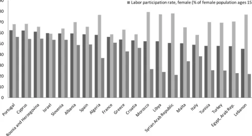
The low labor force participation rates in Turkey present a challenge on her road toward EU accession. As of 2008, Turkey had one of the lowest labor force participation rates among the Organization for Economic Cooperation and Development (OECD) countries ― 48 percent. Turkey is still below 6 percentage points as compared to an average of 54 percent in a group of selected comparison Mediterranean countries that includes EU member and non-member countries. This is due to the very low labor force participation rate of women, in Turkey as seen from Figure 1.
Figure 1. Labor force participation rates: International context
5 Portugal Cyprus
Bosnia and Herzegovina Israel
Slovenia Albania Spain Algeria France Greece Croatia Morocco Libya Syria Malta Italy Tunisia Turkey Egypt 0 10 20 30 40 50 60 0 5000 10000 15000 20000 25000 30000 35000 40000 45000 50000 Fe m al e LF P (% o f fe m al e po pu la ti on a ge s 15 +)
GDP per capita (current US$)
Source: World Development Indicators, 2008
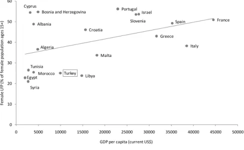
The female labor force participation rate in Turkey was 25 percent as of 2008, whereas this rate was 70 percent for males. The female participation rate in Turkey was 39 and 37 percentage points lower than the EU and OECD average, respectively. Even when compared with the average female labor force participation rate of selected Mediterranean countries included in Figure 1; Turkey was still 15 percent below this 40 percent average. Figure 2 illustrates more clearly this distinctly lower female labor force participation rate in an international context. Among the countries that had a similar GDP per capita as of 2008; Turkey had one of the lowest participation rates for women, together with Syria, Libya, Egypt, Morocco and Tunisia. In the EU member Mediterranean countries, the average female labor force participation rate was 47 with the lowest Malta, 38 percent. Turkey was, still, 22 percentage points below this average.
Figure 2. Femalelabor force participation rates: International context
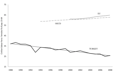
The Turkish Government, on her road toward EU accession, implemented a series of national policies aimed at increasing female labor force participation. The 9th Development Plan has set goals to increase the number of women who are actively employed. Within this framework, the New Labor Act enacted in 2003 examined women’s position in the Turkish labor market and a National Action Plan followed. The National Action Plan for Gender Equality (2008) emphasizes that “using women’s talents and skills in the labor market not only provides families with more economic independence, but also increases women’s self confidence and social respectability”. However, despite all these legislation changes that are likely to have a positive effect on female labor force participation, what is puzzling is depicted in Figure 3 ― the female
6 15 25 35 45 55 65 75 1988 1990 1992 1994 1996 1998 2000 2002 2004 2006 2008 C iv il ia n la bo ur f or ce f em al es % o f po p 15 -64
Source: OECD, Employment and Labour Market Statistics
EU
OECD
TURKEY
labor force participation rate in Turkey has been decreasing, from 37 percent in 1988 to 25 percent in 2008.
Figure 3. Femalelabor force participation rates: 1988-2008
This result is surprising, considering that most of the OECD countries and EU member countries experienced a steady increase in female participation during this period. In 2009, the World Bank published, with the collaboration of the Turkish State Panning Organization, a report that considers “the puzzle of low female labor force participation” in Turkey. The report reveals the two main determinants of this decline: urbanization and the decline in agricultural employment. Urbanization resulted in women migrating from rural areas where they held the status of unpaid family workers in agriculture, to urban areas where they became unpaid household workers. However during these years, Turkey has experienced important structural and social changes that would be expected to facilitate women integration in the labor market: the social attitude toward working women has changed in recent years, women are becoming more educated, women are getting married at a later age, and fertility rates are declining (World Bank, 2009).
The share of illiterate women declined from 33.9 percent to 19.6 percent, and the proportion of university graduate women increased from 1.8 percent to 5.8 over the past 20 years. In addition, the fertility rates in Turkey have been declining since the 1960’s. Women were expected to give birth on average to 5.7 children in 1960; 3 in 1988; and 1.9 in 2008 (World Bank, 2009). Despite these changes that most likely have a positive impact on the female labor force participation rate, its steady decline in the past 20 years is certainly an empirical question. For
7
this reason, the status of women in the Turkish labor market and the barriers to women who are already in the labor force, constitute a central issue and the major motivation of this study.
III. DATA: STRUCTURE OF EARNINGS SURVEY 2006
This study is based on the data given by the Structure of Earnings Survey 2006, Turkish Statistical Institute (TURKSTAT). At present, the Structure of Earnings Survey 2006 is a unique dataset for Turkey, as it provides information on the level, structure and development of wage and earnings. The survey is conducted on a total of 18 232 establishments associated with enterprises with ten or more employees, which were selected by simple random stratified sampling method in overall Turkey. The number of employee records is 308 214 and 77 percent of the employees covered in the survey were males while 23 percent were females. The reference month and year of the survey is November 2006. General information relating to employees is referred to November 2006 and questions on annual payments to employees are referred to the year 2006.
The survey covers employees’ demographic characteristics (age, gender, and education level) and employment variables (occupation, labor status, managerial responsibility, seniority, wages and salaries, working hours) in the survey month and during the year 2006. The variables related to establishments such as size, coverage of collective agreement, as well as the information pertaining to employees throughout the year covering the C-K and M-O sections of the European Union Economic Activity Classification (NACE Rev.1.1) are included in the dataset. The analyses focus on full time employees, comprising 99.3 percent of all employees in the dataset (because the sample size of part time employees is not adequate to achieve reliable statistical inference, we have chosen to consider the more homogeneous group of full-timers). Only workers with type of employment indefinite and fixed term are considered (that is 99 percent of the full time employees), leaving out the paid stagers and apprentices. Furthermore, the sample is restricted to individuals of working age, between 15 and 64 years old.
Table 1 presents the distribution of employees; contractual working hours per week, monthly paid hours, hourly average gross wage, monthly average basic gross wage and monthly average gross wage by sex and educational attainment. The monthly basic gross wage includes the agreed upon and calculated gross wages paid to employees in November 2006 for days worked and not worked, excluding bonuses, premiums, social contributions, and overtime payments,
8
Table 1. Average working hours and monthly average gross wage by sex and educational
attainment
Educational attainment (ISCED,
1997) The distribution of employees Contractual working hours per week Monthly paid hours Hourly average gross wage Monthly average basic gross wage Monthly average gross wage (%) (hours) (TRY) Total 100,0 44,8 197,9 5,2 936 1 023
Primary school and below 30,8 45,1 199,1 3,8 687 750 Primary education and
secondary school 15,5 45,1 199,1 3,8 686 741 High school 23,4 44,9 198,0 4,4 799 864 Vocational high school 10,7 44,8 200,8 5,7 965 1 145 Higher education 19,6 44,1 193,1 9,4 1 673 1 797
Males 100,0 44,9 198,5 5,2 931 1 026
Primary school and below 34,2 45,1 199,2 3,9 700 768 Primary education and
secondary school 16,7 45,1 199,2 3,8 701 762
High school 22,0 44,9 198,6 4,4 805 877
Vocational high school 11,0 44,8 201,8 6,0 995 1203 Higher education 16,1 44,2 194,0 10,1 1786 1931
Females 100,0 44,6 195,6 5,3 955 1 011
Primary school and below 18,8 45,2 198,9 3,2 601 630 Primary education and
secondary school 11,3 45,1 198,5 3,2 602 630 High school 28,3 44,8 196,5 4,3 781 828 Vocational high school 9,3 44,8 196,6 4,6 833 896 Higher education 32,3 43,9 191,5 8,3 1 470 1 557
whereas the monthly gross wage includes the sum of monthly basic wages, overtime payments, payments for shift work/night work and other regular payments paid to employees in November 2006. Monthly paid hours include the sum of contractual working hours pertaining to basic wage and overtime hours worked in November 2006. The hourly wage is calculated by a simple division of monthly wage by monthly paid hours in November 2006.
According to Table 1 female employees covered in the survey are more educated than their male counterparts. The male employees are concentrated in primary school education and below (34 percent), while women are concentrated in higher education (32 percent). The average weekly contractual working hours in Turkey was 44.8. There is not too much variation between education attainment levels and gender in terms of contractual working hours. On the other hand, when the monthly paid hours are compared across gender, there is more variation than in contractual working hours, which in turn implies that males worked more overtime
9
hours in November 2006 relative to their female counterparts in each educational attainment group.
As Table 1 presents, the monthly average gross wage was 1,023 TRY in November 2006, 1,026 and 1,011 TRY for males and females respectively. In other words, women earn 98.5 percent of the wages that men earn on average. It can be seen that the monthly basic wage constitutes more than 90 percent of the monthly gross wage for both genders. When basic wages are compared, we observe that women earn on average 2.5 percentage points more than males. However, in each educational attainment group, the monthly average basic gross wage of females is lower than males’. The higher average female monthly basic wage is the consequence of a composition effect, as women employees are concentrated in the higher education group. As it is clear from the table, there is a direct relation between educational attainment and wages, with wages increasing with education. The hourly average gross wage shows a similar pattern. The distribution of employees by economic activity, firm size, occupational group, type of employment and managerial responsibility is displayed in Table 2. Manufacturing shows the highest concentration of workers for both genders. The wholesalers and retail traders come next. Transport, storage and communication; real estate, renting and business activities; hotels and restaurants are sectors where both genders are almost equally concentrated. 7.5 percent of the female employees work in financial intermediation, a relatively high share when compared with the share of the male employees in this sector, 2.7 percent. Similarly, the mass of male employees is quite low in education, health and social work relative to their female counterparts. On the other hand, mining and quarrying; electricity, gas and water supply; construction seem to be almost exclusively male sectors. In terms of number of employees per firm, the mass of female and male employees are equally concentrated in each firm size group. Most of the employees that are covered in the survey are working in small size firms with 10-49 employees (46.7 percent).
The occupation groups that are covered in the survey are based on the International Standards of Occupation (ISCO, 88). The skilled agricultural and fishery workers constitute only 0.3 percent of the employees in the sample. For this reason, they are considered under the elementary occupations in Table 2 and in the rest of this study. It can be noted that craft and related trade workers; plant and machine operators and assemblers are occupations where males are highly concentrated. On the other hand, 21.8 percent of the female employees are working
10
Table 2. The distribution of employees by gender (%)
Variable Total Males Females
Economic activity (NACE Rev. 1.1) 100,0 100,0 100,0
(C) Mining and quarrying 2,5 3,0 0,7
(D) Manufacturing 42,9 44,5 37,4
(E) Electricity, gas and water supply 3,2 3,7 1,0
(F) Construction 5,2 5,9 2,5
(G) Wholesale and retail trade; repair of motor vehicles, personal and household goods
17,5 16,8 19,7
(H) Hotels and restaurants 4,6 4,6 4,4
(I) Transport, storage and communication 7,6 8,0 6,0
(J) Financial intermediation 3,7 2,7 7,5
(K) Real estate, renting and business activities 6,0 5,7 7,2
(M) Education 2,8 1,9 6,2
(N) Health and social work 2,1 1,1 5,6
(O) Other community, social and personal service activities 2,0 2,0 1,9 Firm Size 100,0 100,0 100,0 10-49 46,7 47,0 45,8 50-249 23,5 23,3 24,2 250-499 10,3 10,3 10,4 500-999 8,1 8,0 8,4 1000+ 11,3 11,3 11,2
Occupational group (ISCO, 88) 100,0 100,0 100,0
1 Legislators, senior officials and managers 5,2 5,3 5,0
2 Professionals 7,1 5,4 13,0
3 Technicians and associate professionals 15,6 14,1 20,7
4 Clerks 10,9 7,9 21,8
5 Service workers and shop and market sales workers
10,6 11,0 9,4
6 Craft and related trade workers 20,7 23,2 11,5
7 Plant and machine operators and assemblers 14,3 16,6 6,0
8 Elementary occupations 15,7 16,5 12,7
Type of employment 100,0 100,0 100,0
Indefinite 95,9 95,6 97,2
Fixed term 4,1 4,4 2,8
Managerial Responsibility 100,0 100,0 100,0
With managerial responsibility 14,7 14,9 14,2
Without managerial responsibility 85,3 85,1 85,8
as clerks and 20.7 of them as technicians and associate professionals. Legislators, senior officials and managers are occupations where both genders are equally concentrated.
For informative purposes, Table 2 includes the distribution of employees with respect to the variable managerial responsibility. 14.7 percent of the employees that are covered in the survey
11
Table 3. Sample means by gender
Total Female Male
Number of observations 302714 65 516 237 198 Hourly wage 5,22 5,27 5,21 (5,80) (5,94) (5,77) P90/P10 3,72 3,72 3,72 P90/P50 3,31 3,34 3,31 P50/P10 1,13 1,11 1,13
Contractual working hrs per week 44,80 44,58 44,86
(2,98) (3,15) (2,92)
Age 32,93 30,53 33,60
(8,57) (8,27) (8,53)
Seniority 3,71 3,03 3,89
(5,21) (4,30) (5,42)
Note: Standard deviations are in paranthesis
had the managerial responsibility as of year 2006. Among men, this share was 14.9, while 14.2 percent of the women employees had the managerial responsibility.
The number of observations that are used in the analyses and the selected descriptive statistics of the relevant variables for this study are presented in Table 3. Table 3 also displays the 90/10, 90/50 and 50/10 percentile ratios of hourly wages for men and women. The smaller the ratio is the more compression takes place. As the 50/10 percentile ratio is quite lower relative to the 90/50 ratio, it can be said that the more compression took place on the lower tail of the wage distribution in November 2006 for both men and women.
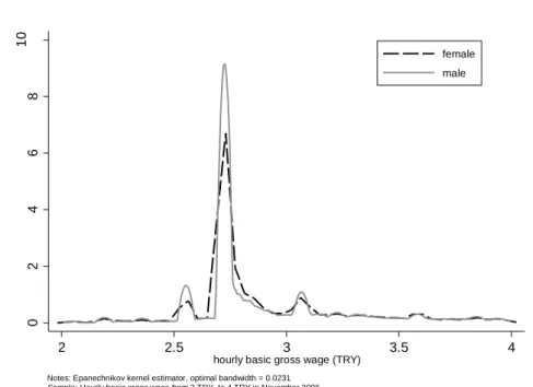
Lastly Figure 4 presents kernel density estimates of the distributions of hourly basic gross wages for females and males, to have a visual summary of the wage distributions. Figure 4 shows the distinction between female’ and males’ wage distributions. The males’ wage distribution peaks relatively high with a lower dispersion around the mode compared to females’. The females’ wage distribution lies within the males’ distribution around the mode. Both genders’ wage distributions peak at the 25th and 75th quantiles and females’ wage distribution lies under the males’ distribution around these quantiles. The two genders’ hourly wage distributions overlap at the upper and lower tail for the interval 2 TRY and 4 TRY.
12
Figure 4. Kernel density estimates of the wage distributions
IV. QUANTILE REGRESSION MODEL
A new growing quantile regression empirical literature shows that the wage distribution needs a more complex analysis than considering the impact of covariates only upon the mean of the conditional wage distribution. The quantile regressions model, introduced by Koenker and Bassett (1978), seeks to extend the analysis to the whole wage distribution and provides a more complete picture of the covariate effects. In this section, the quantile regression method for modeling the wage distributions and the corresponding decomposition technique is discussed. For this purpose, let {𝑦𝑖|𝑖 = 1,2, … , 𝑛} be a random sample of (log) wage units in the population of size 𝑛 with the distribution function 𝐹. For any 𝜃in the interval (0,1) the 𝜃th quantile of the (log) wage distribution can be defined as any number 𝜉𝜃 ∈ ℝthat fulfills:
𝐹𝑌(𝜉𝜃−) = 𝑃(𝑌 < 𝜉𝜃) ≤ 𝜃 ≤ 𝑃(𝑌 ≤ 𝜉𝜃) = 𝐹𝑌(𝜉𝜃). (1)
The smallest element of the solution set to the (1) is chosen to avoid the problems that may arise due to the non-uniqueness problem. Then the quantile function is defined as:
𝑄 𝑌(𝜃) = 𝐹𝑌−1𝑖𝑛𝑓{𝑦| 𝐹𝑌(𝑦) ≥ 𝜃}, 0 < 𝜃 < 1 (2) and the empirical quantile function is:
𝑄̂ 𝑌(𝜃) = 𝐹̂𝑌−1𝑖𝑛𝑓 {𝑦| #(𝑦𝑖≤𝑦) 𝑛 ≥ 𝜃} , 0 < 𝜃 < 1 (3) 0 2 4 6 8 10 D e n s it y 2 2.5 3 3.5 4
hourly basic gross wage (TRY)
female male
Notes: Epanechnikov kernel estimator, optimal bandwidth = 0.0231 Sample: Hourly basic gross wage from 2 TRY to 4 TRY in November 2006
13
𝜉𝜃
Koenker and Bassett (1978) proposed an alternative method to this procedure such that the quantile in question is the solution to the following optimization problem:
𝑄̂ 𝑌(𝜃) = 𝑎𝑟𝑔𝑚𝑖𝑛 [∑𝑖∈{𝑖:𝑦𝑖≥𝜉𝜃}𝜃|𝑦𝑖 − 𝜉𝜃|+ ∑𝑖∈{𝑖:𝑦𝑖<𝜉𝜃}(1 − 𝜃)|𝑦𝑖 − 𝜉𝜃|] (4) This new approach to determine empirical quantiles is convenient for an extension to regression settings. For this purpose let 𝑋 = {𝑥𝑖𝑗|𝑖 = 1,2, … , 𝑛, 𝑗 = 1,2, … , 𝑘} be the matrix of 𝑘 covariates of this sample, which includes a constant, a gender dummy, educational attainment level, age, age squared divided by 100 and seniority. Then the 𝜃th quantile of the (log) wage distribution conditional on the covariates is symbolized as 𝑄𝜃(𝑦𝑖|𝑋) and defined by:
𝑄𝜃(𝑦𝑖|𝑋) = 𝑥𝑖′𝛽(𝜃), 𝜃 ∈ (0,1). (5) where 𝛽(𝜃) is a vector of 𝜃th quantile regression coefficients and 𝑥
𝑖′ is the 𝑖𝑡ℎ row of matrix 𝑋. For a given 𝜃 ∈ (0,1), the quantile regression estimator of 𝛽(𝜃), 𝛽̂(𝜃) is the solution of the following minimization problem (Koenker and Bassett, 1978):
𝛽̂(𝜃) = 𝑎𝑟𝑔𝑚𝑖𝑛 [∑𝑖∈{𝑖:𝑦𝑖≥𝑥𝑖′𝛽(𝜃)}𝜃|𝑦𝑖 − 𝑥𝑖′𝛽(𝜃)|+ ∑𝑖∈{𝑖:𝑦𝑖<𝑥𝑖′𝛽(𝜃)}(1 − 𝜃)|𝑦𝑖 − 𝑥𝑖𝛽(𝜃)|]
= 𝑎𝑟𝑔𝑚𝑖𝑛 ∑ 𝜌𝑖 𝜃(𝑦𝑖− 𝑥𝑖′𝛽(𝜃)) (6)
where 𝜌𝜃(𝑢) = [(𝜃 − Ι(𝑢 < 0))𝑢] is a check function and Ι(∙) is the usual indicator function. In other words, the 𝜃th quantile regression estimator of 𝛽, 𝛽̂(𝜃), can be estimated by minimizing the average of asymmetrically weighted absolute errors, with 𝜃 weight on positive errors and
(𝜃 − 1) on negative errors.
However as the check function is not differentiable at the origin, the minimization problem shown at equation (6) does not have an explicit solution. But it can be shown that the quantile regression can be reformulated in a linear programming representation2. This linear programming representation guarantees the quantile regression estimator to be obtained in a finite number of simplex iterations. The number of simplex iterations is significantly reduced
2 See Buchinsky (1998).
𝛽(𝜃)
14
by the manipulations based on the several equivariance properties of the quantile regression estimator3.
The interpretation of the quantile regression estimator is similar to the least square estimator. Considering the partial derivative of the 𝜃th quantile of the (log) wage distribution conditional on the covariates with respect to one of the regressors, say 𝑗𝑡ℎ, 𝜕𝑄𝜃(𝑦𝑖|𝑋) 𝜕𝑥⁄ 𝑖𝑗 represents the marginal change at the 𝜃th quantile of 𝑦
𝑖 due to a (ceteris paribus) marginal change in the 𝑗th covariate 𝑥𝑖𝑗. The standard errors and confidence intervals for the quantile regression coefficient estimates can be obtained by either using the asymptotic standard error of the estimator or by bootstrapping (Koenker and Hallock, 2000). The elementary asymptotic theory provided by Koenker and Bassett (1978) is based on the assumption of independently and identically distributed errors (𝑖. 𝑖. 𝑑.). In the more realistic case, when the errors are not 𝑖. 𝑖. 𝑑., estimators can be obtained by various re-sampling methods, namely bootstrapping.
V. DECOMPOSITION ANALYSIS USING QUANTILE REGRESSIONS
Following the traditional Oaxaca (1973) decomposition of effects on mean wages, Machado and Mata (2005) proposed a decomposition method combining quantile regressions and the bootstrapping approach. This decomposition method is based on, in the first step, the estimation of the conditional wage distribution by quantile regressions and in the second, the estimation of the marginal density functions of wages that is consistent with the conditional distribution defined by equation (6). For this purpose, Machado and Mata (2005) employed the integral theorem from elementary statistics: if 𝑈 is a uniform random variable on [0,1], then 𝐹−1(𝑈)
has the distribution of 𝐹. Thus if 𝜃1, 𝜃2, … , 𝜃𝑚are randomly drawn from a uniform (0,1) distribution, the 𝑚 estimates of the conditional quantiles at a given 𝑋, {𝑥𝑖′𝛽̂(𝜃𝑖)}𝑖=1
𝑚 will constitute a random sample from the estimated conditional distribution of 𝑦𝑖 at given 𝑋. Then, to get a sample from the marginal, rather than keeping 𝑋 fixed, a random sample of the covariates can be drawn from the population. Formally, the steps of this procedure can be summarized as:
1. Generate a random sample of size m from a 𝑈[0,1]: 𝜃1, 𝜃2, … , 𝜃𝑚.
3 See Koenker and Bassett (1978), Buchinsky (1998), Koenker and Hallock (2000) for equivariance properties of the quantile regression estimator.
15
2. For the data set and each {𝜃𝑖}𝑖=1𝑚 estimate 𝑄𝜃𝑖(𝑦|𝑋) to get 𝑚 estimates of quantile regression coefficients 𝛽̂(𝜃𝑖), 𝑖 = 1,2, … , 𝑚.
3. Generate a random sample of size 𝑚 with replacement from the covariates, denoted by
{𝑥̃𝑖}𝑖=1𝑚 .
4. Finally {𝑦̃𝑖 = 𝑥̃𝑖′𝛽̂(𝜃𝑖)}𝑖=1𝑚 is a random sample of size 𝑚 from the desired distribution. In particular we are interested in two types of counterfactual wage distribution, males’ and females’. In other words, to reveal the gender wage gap, we want to simulate the marginal wage distribution that would have prevailed for females if all covariates had been distributed as males’. In this case the above procedure is run as:
1. Generate a random sample of size m from a 𝑈[0,1]: 𝜃1, 𝜃2, … , 𝜃𝑚.
2. For the data set and each {𝜃𝑖}𝑖=1𝑚 estimate the quantile regression coefficients: 𝛽̂𝑓𝑒𝑚𝑎𝑙𝑒(𝜃
𝑖) ,
𝛽̂𝑚𝑎𝑙𝑒(𝜃𝑖), 𝑖 = 1,2, … , 𝑚 , for females and males respectively.
3. Generate for each gender a random sample of size m with replacement from the covariates, denoted by {𝑥̃𝑖𝑓𝑒𝑚𝑎𝑙𝑒} 𝑖=1 𝑚 and {𝑥̃𝑖𝑚𝑎𝑙𝑒} 𝑖=1 𝑚 . 4. {𝑦̃𝑖𝑓𝑒𝑚𝑎𝑙𝑒 = 𝑥̃𝑖𝑓𝑒𝑚𝑎𝑙𝑒′𝛽̂𝑓𝑒𝑚𝑎𝑙𝑒(𝜃 𝑖)} 𝑖=1 𝑚 and {𝑦̃𝑖𝑚𝑎𝑙𝑒 = 𝑥̃𝑖𝑚𝑎𝑙𝑒 ′𝛽̂𝑚𝑎𝑙𝑒(𝜃 𝑖)} 𝑖=1 𝑚 are random samples of size 𝑚 from the marginal wage distributions consistent with the linear model defined in equation (5).
5. Generate a random sample of the counterfactual distribution. {𝑥̃𝑖𝑚𝑎𝑙𝑒′𝛽̂𝑓𝑒𝑚𝑎𝑙𝑒(𝜃𝑖)}
𝑖=1 𝑚
is a random sample from the wage distribution that would have prevailed for females if all covariates had been distributes as males’.
The step 5 can be repeated to generate the second counterfactual density by simply reversing the roles of females and males. This way, two counterfactual densities are obtained: (1) the female log wage density that would arise if women were given men’s characteristics but having their own wages and (2) the density that would arise if women retained their own characteristics but were paid like their male counterparts (Albrecht, et al., 2003).
Then the decomposition of the difference between quantiles of the male and female wage distribution is given by:
16
where the first component is the contribution of the covariates and the second component is the contribution of the coefficients to the difference between the 𝜃th quantile of the male wage distribution and the 𝜃th quantile of the female wage distribution.
VI. RESULTS FROM QUANTILE REGRESSION AND DECOMPOSITION
ANALYSIS
In this section the results from quantile regression estimates and the decomposition of observed gender wage gaps are presented. Firstly, following Albrecht et al. (2003), for various specifications, a series of quantile regression estimations is performed to explore the gender gap that remains unexplained at the various quantiles of the wage distribution by using the pooled dataset of males and females. Secondly, the quantile regressions for females and males are estimated separately and the difference between returns of individual and firm characteristics at the various points in female and male wage distributions is presented. Lastly, the decomposition results of the difference between the male and female wage distribution is displayed.
Pooled Quantile Regression Results with Gender Dummies
In this part of the analyses, a series of quantile regressions are estimated using the total male and female mixed sample. The coefficient estimates and the standard errors of the gender dummy in each specification for the fifth, tenth, twenty-fifth, fiftieth, seventy-fifth, ninetieth and ninety-fifth percentiles are presented in Table 4. The standard errors of the quantile regression coefficients in parentheses are obtained by bootstrapping method4. For comparison,
the OLS estimate of the gender dummy coefficient in each model is displayed in the last column of the Table 4. The gender dummy coefficients in Table 4 present the gender gap that remains unexplained at the various quantiles of the wage distribution after controlling for the covariates
4 Among the commercial software packages, Stata provides basic functionalities to estimate the quantile regression estimators and their standard errors. The command qreg provides the asymptotic standard errors based on the assumption of 𝑖. 𝑖. 𝑑. errors. In particular, the reported standard errors in this study are based on the pair wise bootstrapping where pairs, (𝑦𝑖, 𝑥𝑖)𝑖 = 1,2, … , 𝑛, are randomly drawn from the original sample with replacement. As the observations of our analyses come from a simple random stratified sampling method, the pair wise bootstrapping approach, which is based on the independently but not identically distributed setting, is consistent. For this purpose, the command for simultaneous quantile regressions sqreg is used and the re-sampling procedure is repeated 100 times, to yield a sample whose covariance matrix is a consistent estimator of the covariance matrix of the original estimator.
17
in each specification. A negative coefficient implies that a negative unexplained gender gap remains even after the labor market characteristics in the model are controlled for. The lower the coefficient is, the more disadvantageous the women are. On the other hand, expanding the controls from one model to another, aims at exploring the change in the gender dummy coefficient from the simplest model to the expanded model in various quantiles.
The first specification named as observed gender gap is the basic model where log hourly wage is regressed on the gender dummy. Basic control variables include the individual specific characteristics, such as age, age square divided by 100, seniority and educational attainment. Extended controls further include the employment type variable. Firm characteristics include the size and the coverage of the workplace under collective labor bargaining. The eight occupation dummies are based on one-digit classification and the twelve economic activity dummies are based on the two digit classification.
When the rows of the Table 4 are compared, it can be seen that expanding the model has an impact on the gender dummy coefficient. Firstly, the comparison of second and third rows of the Table 4 suggests that adding employment type to the model has no clear impact on the gender gap at the lower quantiles. At the upper tail of the wage distribution, the gender gap slightly increases after adding employment type as a control variable. Secondly, the pair wise comparison of the third and fourth models in Table 4 shows that, when economic activity is controlled for, the gender wage gap at the upper tail of the wage distribution (90th and 95th quantiles) increases. Conversely, including economic activity as an explanatory variable decreases the gap at the median and at the 75th quantile. Moreover, adding occupation as a control variable increases the gender wage gap, as revealed by the pair wise comparison of models four and five at each quantile in which this coefficient is significant. On the other hand, the OLS coefficient suggests that there is no effect of controlling for employment type and occupation at the mean of the wage distribution. The fifth and sixth models comparison suggest that controlling for the firm characteristics increases the gap at the bottom and the median, as well as the mean, while decreasing it at the top of the wage distribution.
One of the striking features of the results in Table 4 is that the gender dummy coefficient is decreasing in each model, except the first specification, as the quantile increases. In other words, the gender wage gap that remains unexplained is higher in the upper tail of the wage distribution than at the median and the lower tail. In the first specification, where none of the controls are taken into account, women seem to be positively discriminated in the upper tail.
18 Table 4. Gender dummy coefficients using alternative specifications
Specification Quantile regressions (percentage of the conditional wage distribution) OLS
5th 10th 25th 50th 75th 90th 95th mean
(1) Observed gender gap 0,000 0,000 0,000 -0,010** -0,018** 0,002 0,074*** -0,002
(0,000) (0,000) (0,000) (0,004) (0,008) (0,007) (0,008) (0,003)
(2) Gender gap with basic control variables -0,000 -0,000 -0,009*** -0,024*** -0,058*** -0,077*** -0,067*** -0,051***
(0,001) (0,000) (0,001) (0,001) (0,002) (0,004) (0,007) (0,002)
(3) Gender gap with extended control variables -0,000 -0,000 -0,010*** -0,023*** -0,058*** -0,078*** -0,069*** -0,051***
(0,001) (0,000) (0,001) (0,001) (0,002) (0,004) (0,006) (0,002)
(4) Gender gap with extended control variables and sector -0,000 -0,001* -0,009*** -0,019*** -0,056*** -0,082*** -0,082*** -0,055***
(0,001) (0,000) (0,001) (0,001) (0,002) (0,004) (0,007) (0,002)
(5) Gender gap with extended control variables, sector and occupation -0,000 -0,002*** -0,010*** -0,023*** -0,058*** -0,095*** -0,096*** -0,055***
(0,001) (0,001) (0,001) (0,001) (0,002) (0,004) (0,007) (0,002)
(6) Gender gap with extended control variables, sector, occupation and firm
characteristics -0,006*** -0,007*** -0,014*** -0,024*** -0,043*** -0,062*** -0,075*** -0,047***
(0,001) (0,001) (0,001) (0,001) (0,002) (0,004) (0,005) (0,002)
Source: TUIK, Structure of Earnings Survey, 2006.
Note: Standard errors are in parentheses. For quantile regressions bootstrapped standard errors (100 replications) are reported.
*, ** and *** significant at 1, 5 and 10 % significance level respectively
1. Observed gender gap includes gender dummy without any control variables. Basic control variables include age, age2/100, and seniority and education level. Extended controls include additional to basic
controls dummy for employment type. Firm characteristics are firm size and cover of collective bargaining.
2. 8 major occupation group (ISCO, 88) dummies are: 1. Legislators, senior officials and managers, 2. Professionals, 3. Technicians and associate professionals, 4. Clerks, 5. Service workers and shop and market
sales workers, 6. Craft and related trade workers, 7. Plant and machine operators and assemblers, 8. Elementary occupations
3 12 economic activity (NACE Rev. 1.1) dummies are: 1. Mining and quarrying, 2. Manufacturing , 3. Electricity, gas and water supply, 4. Construction, 5. Wholesale and retail trade; repair of motor vehicles,
motorcycles and personal and household goods, 6. Hotels and restaurants, 7. Transport, storage and communication, 8. Financial intermediation, 9. Real estate, renting and business activities, 10. Education, 11. Health and social work, 12. Other community, social and personal service activities
19
However, when we start to control for relevant labor market characteristics, this result is reversed, already after the basic controls (second row of Table 4). This effect, as described in Section III, is a consequence of the composition of employees. As women are concentrated in the higher education groups, the observed raw gender gap suggests that women are positively discriminated at the upper tail of the wage distribution.
Another salient feature of the results displayed in Table 4 is the insignificance of the gender dummy coefficient for the fifth percentile in most of the models, and for the tenth in some, except the one that controls for the firm characteristics (6th row of Table 4). This implies that there is no significant evidence for a gender wage gap at the lowest quantile of the wage distribution when firm characteristics are not controlled for. Despite the gender dummy not being significant at the 5th quantile in any model, the coefficient turns significant already from the 25th quantile onwards. When the firm characteristics are added to the controls, interestingly, the gender wage gap increases in the lower quantiles, namely, 5th, 10th and 25th while it is reduced in absolute terms in higher, 90th and 95th, quantiles. Considering the significant effect of the firm characteristics to the marginal effect of gender dummy on log wage distribution, in the further steps of the analyses the last specification in Table 4 is preferred. In so doing, we are able to control observed firm specific factors, which have a significant effect on the magnitude of the gender wage gap along the wage distribution.
Lastly, the equality of the gender dummy coefficients is tested for various combinations of quantile pairs in each model presented in table 4. In all specifications, the equality of the seven gender dummy coefficients is rejected at one percent significance level. Furthermore, in all models, except the last two, the gender dummy coefficient at the 5th-10th and 90th-95th quantile pairs are not statistically different, at the 1% significance level. The difference between gender dummy coefficients at the 90th and 95th quantiles in the fifth model is not statistically significant, while in the sixth specification this difference is not statistically significant only at the 5th and 10th quantiles.
On the other hand, the estimated OLS coefficient for gender dummy is between – 4.7% and -5.5% if we consider all the specifications from the second to the sixth. For each specification this coefficient is close to the one that is estimated from the 75th quantile regression. However, the coefficients at the lowest and highest quantiles, even at the median, are quite different than the OLS estimates. In other words, OLS estimates are not sufficient to capture the marginal effect of the gender dummy on log hourly wages at the lower and the upper tails of the wage distribution, irrespective to the specification.
20
The complete set of quantile regression and OLS estimates of the coefficients for regression on the extended control variables, sector, and occupation as well as firm characteristics is displayed in Table 55. As Table 5 presents, the effects of age and age square on log hourly wages are constant at the 5th, 10th and 50th quantile, whereas it increases at the upper tail of the distribution. The marginal effect of seniority on wages is 0.7 % at the 5th quantile and 10th quantiles. This effect increases to around 3 % at the upper tail of the wage distribution. At each quantile, estimated returns to education increase with the level of education. The same applies for the OLS estimation results. For instance, the wage of an employee who completed the primary education or attended a secondary school is 0.7% higher than for a worker who either attended primary school or no school, at the 5th quantile, controlling for age, gender, seniority, education, occupation and sector as well as firm characteristics. Whereas this difference is 5.4 percentage points between a university graduate and a worker who either attended primary school or no school. Similarly, at the 95th quantile this difference turns to be 9.8% for an employee who completed the primary education or attended a secondary school and 93.4% for a university graduate. Then again, at each education level, estimated returns to education are similar for the lower quantiles, while it starts to increase at the median noticeably and continue to increase as we move up the wage distribution.
The coefficient of the fixed term employment is – 0.024 at the 5th quantile while it is – 0.001 at the median and – 0.063 at the highest quantile. This implies that employees working with a fixed term contract are earning 2.4 percentage points less than the ones who are working with an indefinite contract at the 5th quantile, controlling for age, seniority, education, occupation and sector as well as firm characteristics. The fixed term penalty decreases through the wage distribution up to median but start to increase after it as we move up to the upper tail of the wage distribution.
Moreover at each quantile, there is a pay advantage of workers who work in large workplaces. Accordingly, of two workers with the same gender, age, seniority, level of education, type of contract, working in the same sector and occupation, and both covered with the collective labor agreement, the one in the largest workplace earns 10.6% more than the one in a workplace with less than 50 employees at the 5th quantile. This gap is 32.6% at the median and 43.6% at the highest quantile.
5 The complete set of estimations in the rest of the specifications are presented in Tables A.1, A.2, A.3 and A.4 in appendix.
21 Table 5. Pooled quantile regressions with gender dummy
Variables Quantile regressions (percentage of the conditional wage distribution) OLS
5th 10th 25th 50th 75th 90th 95th mean Female -0,006*** -0,007*** -0,014*** -0,024*** -0,043*** -0,062*** -0,075*** -0,047*** (0,001) (0,001) (0,001) (0,001) (0,002) (0,004) (0,005) (0,002) Age 0,002*** -0,000 -0,001*** 0,003*** 0,011*** 0,032*** 0,046*** 0,023*** (0,000) (0,000) (0,000) (0,000) (0,001) (0,001) (0,002) (0,001) Age2/100 -0,001** 0,001*** 0,002*** -0,002*** -0,010*** -0,028*** -0,042*** -0,022*** (0,001) (0,000) (0,000) (0,000) (0,001) (0,002) (0,003) (0,001) Seniority 0,007*** 0,007*** 0,013*** 0,025*** 0,034*** 0,033*** 0,032*** 0,026*** (0,000) (0,000) (0,000) (0,000) (0,000) (0,000) (0,001) (0,000)
Primary education and
secondary school 0,007*** 0,006*** 0,011*** 0,018*** 0,042*** 0,085*** 0,098*** 0,049***
(0,001) (0,001) (0,001) (0,001) (0,002) (0,004) (0,007) (0,002)
High school 0,014*** 0,010*** 0,016*** 0,026*** 0,067*** 0,154*** 0,207*** 0,084***
(0,001) (0,001) (0,001) (0,001) (0,002) (0,004) (0,006) (0,002)
Vocational high school 0,035*** 0,032*** 0,038*** 0,071*** 0,186*** 0,276*** 0,336*** 0,173***
(0,002) (0,001) (0,001) (0,002) (0,004) (0,005) (0,008) (0,003)
Higher education 0,054*** 0,056*** 0,078*** 0,342*** 0,617*** 0,823*** 0,934*** 0,447***
(0,002) (0,001) (0,001) (0,006) (0,006) (0,010) (0,011) (0,003)
Fixed term employment -0,024*** -0,008*** -0,002 -0,001 -0,016*** -0,051*** -0,063*** -0,029***
(0,006) (0,002) (0,001) (0,002) (0,003) (0,006) (0,009) (0,004) 50-249 employees 0,040*** 0,022*** 0,029*** 0,045*** 0,164*** 0,234*** 0,235*** 0,151*** (0,001) (0,001) (0,001) (0,001) (0,003) (0,005) (0,006) (0,002) 250-499 employees 0,067*** 0,052*** 0,058*** 0,148*** 0,307*** 0,344*** 0,311*** 0,256*** (0,001) (0,001) (0,001) (0,003) (0,004) (0,005) (0,009) (0,003) 500-999 employees 0,085*** 0,066*** 0,074*** 0,197*** 0,344*** 0,358*** 0,326*** 0,290*** (0,001) (0,001) (0,002) (0,004) (0,005) (0,006) (0,008) (0,003) 1000+ employees 0,106*** 0,089*** 0,209*** 0,326*** 0,440*** 0,461*** 0,436** 0,376*** (0,002) (0,001) (0,004) (0,004) (0,006) (0,007) (0,008) (0,003) Collective agreement 0,124*** 0,227*** 0,418*** 0,384*** 0,270*** 0,229*** 0,210*** 0,258*** (0,003) (0,005) (0,004) (0,004) (0,005) (0,006) (0,007) (0,003) Constant 0,866*** 0,936*** 1,033*** 1,282*** 1,483*** 1,391*** 1,300*** 0,901*** (0,009) (0,005) (0,006) (0,011) (0,014) (0,026) (0,035) (0,012) Number of observations 302 714 302 714 302 714 302 714 302 714 302 714 302 714 302 714 Pseudo-R2 0,06 0,07 0,15 0,33 0,43 0,42 0,41 0,53 Source: TUIK, Structure of Earnings Survey, 2006.
Note: Standard errors are in parentheses. For quantile regressions bootstrapped standard errors (100 replications) are reported. *, ** and *** significant at 1, 5 and 10 % significance levels respectively
1.The regressions include 8 major occupation group (ISCO, 88) dummies: 1. Legislators, senior officials and managers, 2. Professionals,
3. Technicians and associate professionals, 4. Clerks, 5. Service workers and shop and market sales workers, 6.Craft and related trade workers, 7. Plant and machine operators and assemblers, 8. Elementary occupations
2.The regressions include 12 economic activity (NACE Rev. 1.1) dummies: 1. Mining and quarrying, 2. Manufacturing , 3. Electricity,
gas and water supply, 4. Construction, 5. Wholesale and retail trade; repair of motor vehicles, motorcycles and personal and household goods, 6. Hotels and restaurants, 7. Transport, storage and communication, 8. Financial intermediation, 9. Real estate, renting and business activities, 10. Education, 11. Health and social work, 12. Other community, social and personal service activities
22
If a similar analysis is performed for the coefficient estimate of the coverage of the workplace under collective labor agreement, there is a pay advantage for the workers who are working in a workplace that is under the collective labor agreement. The highest is at 25th quantile of the wage distribution with 41.8% difference and second at the median with 38.4%. The lowest difference exists at the bottom and the top of the difference, 12.4% and 21% at the 5th and 95th quantiles, respectively.
Quantile Regression Results by Gender
In the analyses, the quantile regressions are estimated separately for females and males to examine if a difference between the returns to individual and firm characteristics for women and men exists at the various points of their respective wage distributions. Table 6 displays the estimated coefficients of the extended control variables, such as age, age squared, seniority, education and type of contract, as well as the firm characteristics, by the quantile log wage regressions separately for males and females at various quantiles.
For both genders, the coefficients on age are higher at the upper tail of the wage distribution than the lower tail and the median while for women these coefficients are higher than for men at all the quantiles of the wage distribution. An additional year of seniority is associated with a similar increase in pay for males and females at the lower tail of the wage distribution, at the median and at the 75th quantile. However at the upper tail of the distribution there is a pay advantage of women who have an additional year of seniority than men around 0.4% at the 90th quantile and 0.7% at the 95th quantile. On the other hand women get a higher return to education than men at all the quantiles for the primary education level. The same applies for the high school graduates. In contrast, among vocational high school and university graduates, men realize higher return to education than women at the lower tail and the median of the wage distribution. For vocational high school graduates at the 75th quantile, for the higher education level at the 95th quantile women start to get a bigger payoff than men.
The coefficient of the fixed term employment is – 0.016 and – 0.044 at the 5th quantile while it is – 0.049 and – 0.054 at the 90th quantile for men and women respectively. This implies that female employees that are working with a fixed term contract are earning 0.5% less than their male counterparts at the 90th quantile. This gap is even higher at the lower quantiles, with 2.8% at the 5th quantile.
23 Table 6. Quantile regressions by gender
Variables
Quantile regressions (percentage of the conditional wage distribution) O OLS
5th 10th 25th 50th 75th 90th 95th mean
Male Female Male Female Male Female Male Female Male Female Male Female Male Female Male Female
Age 0,001* 0,004*** -0,001** 0,002*** -0,002*** 0,003*** 0,001*** 0,009*** 0,006*** 0,027*** 0,028*** 0,049*** 0,041*** 0,061*** 0,019*** 0,038*** (0,001) (0,001) (0,000) (0,001) (0,000) (0,001) (0,000) (0,001) (0,001) (0,001) (0,001) (0,003) (0,002) (0,004) (0,001) (0,001) Age2 -0,000 -0,005*** 0,002*** -0,002*** 0,004*** -0,003*** -0,000 -0,011***** -0,004*** -0,032*** -0,024*** -0,054*** -0,036*** -0,063*** -0,017*** -0,042*** (0,001) (0,001) (0,000) (0,001) (0,000) (0,001) (0,000) (0,001) (0,001) (0,002) (0,002) (0,004) (0,003) (0,007) (0,001) (0,002) Seniority 0,007*** 0,006*** 0,007*** 0,006*** 0,013*** 0,012*** 0,025*** 0,025*** 0,033*** 0,033*** 0,033*** 0,037*** 0,030*** 0,037*** 0,025*** 0,026*** (0,000) (0,000) (0,000) (0,000) (0,000) (0,001) (0,000) (0,001) (0,000) (0,001) (0,001) (0,001) (0,001) (0,002) (0,000) (0,000) Primary education
and secondary school 0,006*** 0,010*** 0,006*** 0,011*** 0,010*** 0,018*** 0,016*** 0,035*** 0,033*** 0,091*** 0,067*** 0,155*** 0,084*** 0,193*** 0,041*** 0,108***
(0,002) (0,003) (0,001) (0,002) (0,001) (0,002) (0,001) (0,002) (0,002) (0,005) (0,004) (0,009) (0,007) (0,013) (0,003) (0,007) High school 0,012*** 0,015*** 0,010*** 0,014*** 0,013*** 0,024*** 0,021*** 0,043*** 0,050*** 0,124*** 0,131*** 0,230*** 0,175*** 0,308*** 0,069*** 0,139*** (0,002) (0,003) (0,001) (0,002) (0,001) (0,002) (0,001) (0,002) (0,003) (0,006) (0,006) (0,012) (0,008) (0,015) (0,002) (0,006) Vocational high school 0,040*** 0,013*** 0,036*** 0,016*** 0,038*** 0,033*** 0,072*** 0,064*** 0,177*** 0,210*** 0,268*** 0,298*** 0,331*** 0,355*** 0,168*** 0,189*** (0,002) (0,004) (0,001) (0,002) (0,001) (0,002) (0,003) (0,003) (0,005) (0,012) (0,007) (0,016) (0,010) (0,020) (0,003) (0,008) Higher education 0,055*** 0,046*** 0,057*** 0,049*** 0,091*** 0,067*** 0,380*** 0,281*** 0,641*** 0,590*** 0,828*** 0,819*** 0,938*** 0,942*** 0,458*** 0,437*** (0,002) (0,004) (0,001) (0,003) (0,004) (0,003) (0,006) (0,008) (0,008) (0,012) (0,010) (0,016) (0,014) (0,017) (0,003) (0,007) Fixed term employment -0,016** -0,044*** -0,004** -0,021*** 0,002 -0,019*** -0,000 -0,005 -0,013*** -0,029*** -0,049*** -0,054** -0,078*** 0,014 -0,025*** -0,059*** (0,007) (0,008) (0,002) (0,004) (0,002) (0,005) (0,002) (0,005) (0,003) (0,007) (0,006) (0,018) (0,010) (0,027) (0,004) (0,010) 50-249 employees 0,040*** 0,043*** 0,020*** 0,025*** 0,027*** 0,035*** 0,042*** 0,053*** 0,186*** 0,104*** 0,252*** 0,154*** 0,252*** 0,169*** 0,150*** 0,159*** (0,002) (0,003) (0,001) (0,001) (0,001) (0,002) (0,001) (0,002) (0,004) (0,005) (0,005) (0,010) (0,008) (0,012) (0,002) (0,004) 250-499 employees 0,068*** 0,063*** 0,051*** 0,050*** 0,056*** 0,060*** 0,164*** 0,112*** 0,340*** 0,199*** 0,371*** 0,227*** 0,338*** 0,220*** 0,262*** 0,239*** (0,002) (0,003) (0,002) (0,002) (0,001) (0,003) (0,004) (0,006) (0,006) (0,010) (0,007) (0,013) (0,009) (0,015) (0,003) (0,006) 500-999 employees 0,087*** 0,081*** 0,068*** 0,059*** 0,081*** 0,064*** 0,226*** 0,118*** 0,377*** 0,228*** 0,381*** 0,272*** 0,352*** 0,258*** 0,302*** 0,261*** (0,002) (0,003) (0,001) (0,002) (0,002) (0,003) (0,005) (0,007) (0,005) (0,013) (0,007) (0,017) (0,010) (0,019) (0,003) (0,007) 1000+ employees 0,111*** 0,097*** 0,097*** 0,073*** 0,235*** 0,121*** 0,360*** 0,218*** 0,482*** 0,282*** 0,495*** 0,298*** 0,470*** 0,307*** 0,395*** 0,312*** (0,002) (0,003) (0,002) (0,002) (0,005) (0,008) (0,005) (0,007) (0,006) (0,013) (0,009) (0,017) (0,011) (0,017) (0,003) (0,006)
24 Collective agreement 0,134*** 0,080*** 0,250*** 0,122*** 0,426*** 0,286*** 0,375*** 0,345*** 0,259*** 0,268*** 0,225*** 0,216*** 0,211*** 0,200*** 0,258*** 0,221*** (0,003) (0,007) (0,007) (0,011) (0,005) (0,012) (0,004) (0,010) (0,005) (0,012) (0,006) (0,022) (0,007) (0,022) (0,003) (0,008) Constant 0,873*** 0,857*** 0,943*** 0,916*** 1,049*** 0,984*** 1,284*** 1,243*** 1,526*** 1,296*** 1,416*** 1,121*** 1,356*** 0,989*** 0,962*** 0,663*** (0,010) (0,019) (0,005) (0,010) (0,006) (0,017) (0,012) (0,035) (0,016) (0,045) (0,027) (0,063) (0,039) (0,099) (0,014) (0,033) Number of observations 237 198 65 516 237 198 65 516 237 198 65 516 237 198 65 516 237 198 65 516 237 198 65 516 237 198 65 516 237 198 65 516 Pseudo-R2 0,06 0,05 0,08 0,04 0,17 0,11 0,35 0,28 0,44 0,40 0,43 0,41 0,42 0,41 0,54 0,48
Source: TUIK, Structure of Earnings Survey, 2006.
Note:Standard errors are in parentheses. For quantile regressions bootstrapped standard errors (100 replications) are reported. *, ** and *** significant at 1, 5 and 10 % significance levels respectively
1.The regressions include 9 major occupation group (ISCO, 88) dummies: 1. Legislators, senior officials and managers, 2. Professionals, 3. Technicians and associate professionals, 4. Clerks, 5. Service workers and shop and market sales
workers, 6. Craft and related trade workers, 7. Plant and machine operators and assemblers, 8. Elementary occupations
2.The regressions also include 12 economic activity (NACE Rev. 1.1) dummies: 1. Mining and quarrying, 2. Manufacturing, 3. Electricity, gas and water supply, 4. Construction, 5. Wholesale and retail trade; repair of motor vehicles,
motorcycles and personal and household goods, 6. Hotels and restaurants, 7. Transport, storage and communication, 8. Financial intermediation, 9. Real estate, renting and business activities, 10. Education, 11. Health and social work, 12. Other community, social and personal service activities
25
In terms of firm characteristics, first, women have a pay penalty in large firms with more than 500 employees. In the small and medium size firms, at the lower tail of the wage distribution men have a pay penalty, but men start to get a bigger payoff than women at the small size firms starting from the 75th quantile and at firms with 250-499 employees starting from the median. Second, after controlling for the age, seniority, level of education, type of contract, sector and occupation, and size of the workplace, male employees have a pay advantage than women in workplaces those covered under collective bargaining agreements, except the 75th quantile at which women have an advantage of 0.9%.
The OLS estimates of the coefficients are reported in the last two columns of Table 6. It is clear that, OLS is not adequate to analyze these patterns of differences between the returns of individual and firm characteristics at the various points of female and male wage distributions.
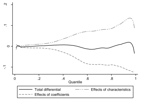
Decomposition Results for Gender Wage Gap Using Quantile Regressions
So far we have dealt with the quantile regression estimates but now we turn our attention to the decomposition of the observed gender gap into two components: one due to the characteristics and the other to the coefficients6. Given the size of the dataset and the computational limitations, it was
not feasible to perform the decomposition on the whole sample. Therefore, in this part of the analysis a random sample of the data consisting of 20% of the whole data set is used.
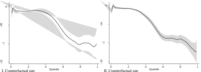
For decomposition analyses, first, the counterfactual densities for several alternative specifications are constructed assuming that women have the male labor market characteristics but are rewarded for these characteristics as female employees. Table 7 shows the counterfactual gap that is the gap between male log wage density and the counterfactual density for several alternative specifications presented in the previous section. The first row of the Table 7 gives the observed gender gap at the various quantiles of the wage distribution that is identical to the one in Table 4. The counterfactual gender gaps in Table 7 are the gaps between male log wage densities and the counterfactual densities constructed by estimating the betas using only women and then assuming that women have the male distribution of labor market characteristics.
6 The decomposition of differences in wage distributions is applied using the Stata command rqdeco (See Melly, 2007). Melly (2006) shows that this procedure is numerically identical to the Machado and Mata (2005) decomposition method when the number of simulations used in Machado and Mata procedure goes to infinity. In the decomposition procedure of our study, rather than taking 𝑚 random draws from (0,1) and estimating 𝑚 quantile regression coefficients, the decomposition is performed for the 99 percentile differences in wages between men and women. 100 quantile regressions are estimated in the first step and the standard errors for the counterfactual densities are obtained by repeating the procedure 100 times.