D
ISSERTATION
Statistical analysis of concentration-dependent
high-dimensional gene expression data
Submitted to
the Department of Statistics
of the University of Dortmund
in Fulfillment of
the Requirements for the Degree of
Doktor der Naturwissenschaften
By
Marianna Grinberg
Dortmund, June 2017
Referees:
Prof. Dr. Jörg Rahnenführer
Prof. Dr. Guido Knapp
Prof. Dr. J. Hengstler
1 Introduction 1
2 Biological background 4
2.1 Central dogma of molecular genetics . . . 4
2.2 Affymetrix GeneChip Technology . . . 6
2.3 Data Preprocessing . . . 9
2.4 Data sets . . . 13
2.4.1 TG-GATEs database . . . 13
2.4.2 UKN1 test system . . . 17
2.4.3 NRW database . . . 18
3 Statistical methods 20 3.1 Principal component analysis . . . 20
3.2 Heatmap . . . 24
3.3 Limma: LinearModels forMicroarray Data . . . 26
3.4 Statistics for concentration-dependent analyses . . . 29
3.4.1 Progression profile index . . . 29
3.4.2 Progression profile error indicator . . . 30
3.4.3 Modified progression profile error indicator . . . 30
3.4.4 Selection value . . . 30
3.4.5 Overlap ratio . . . 31
3.5 Dose-response theory . . . 32
3.5.1 Four-parameter log-logistic model (4pLL) . . . 33
3.5.2 Re-parametrization of the EC50 . . . 34
3.5.3 The ALEC and its confidence interval . . . 35
ii Contents
3.5.5 Test statistic for the effect level . . . 38
3.5.6 Lowest Effective Concentration (LEC) . . . 39
3.5.7 Measures of toxicity . . . 41
4 Toxicogenomics directory of chemically exposed human hepatocytes 43 4.1 Batch effects . . . 43
4.2 Reproducibility . . . 44
4.3 Number of deregulated genes . . . 46
4.4 Concentration progression . . . 48
4.5 Stereotypic versus compound-specific gene expression responses . . . 55
4.6 Unstable baseline genes . . . 58
4.7 Further analyses . . . 58
5 Consensus gene signature of rat hepatocytes tested in in vitro and in in vivo test systems 60 5.1 Data structure of the NRW database . . . 60
5.2 Consensus signature . . . 71
5.3 Data structure of the TG-GATEs database . . . 76
6 Statistical analysis of dose-expression data 84 6.1 Simulation study and setup . . . 84
6.2 Results of the simulation study . . . 87
6.2.1 Comparison of the distributions . . . 87
6.2.2 Comparison of the quantile distributions . . . 95
6.2.3 Comparison of the deviations . . . 96
6.2.4 Direct comparison of the two estimates . . . 98
6.3 Results of a real data study . . . 107
7 Summary 114
Bibliography 119
List of Figures 1
A Derivation 6 A.1 Derivation of∇h(φ) . . . 6 A.2 Derivation of∇f(x, φ) . . . 7 A.3 Derivation ofγ =F(tν) . . . 8 B Tables 9 C Figures 35
1 Introduction
Understanding the behavior of genes as a response to external influences, such as radiation or chemicals, on a fundamental level is one of the great challenges of modern biology. In specific, the investigation of chemically-induced toxicity is of major importance since it is crucial for the identification of biomarkers and the development of drugs. One approach to accomplish this objective utilizes toxicogenomics which is based upon the combination of toxicology and the analysis of genome-wide gene expression data. This research field uses the technology of microarrays which allows the simultaneous measurement of the expression of tens of thousands of genes. Nowadays, toxicogenomics has evolved to an established practice in the still emerging field of chemical hazard identification. It comprises the analysis of large-scale gene expression data in order to identify and characterize different modes of action associated with certain expression changes. Such deregulations, which occur as a response to chemical exposure, provide initial evidence of the involved toxic mechanisms. Based upon it, the key aspect is to detect those genes which improve the understanding of molecular mechanisms on a protein level. It is this particular understanding of the linkage between the entirety of all genes, transcriptome, proteome and eventually metabolome which qualifies for the assessment of biological processes within the human organism. Hence, especially the pharmaceutical sector applies the methods used within toxicogenomics for the research on drugs and, here, particularly the correct dosage is of vital importance.
Often, concentrations that cause gene alterations are associated with adverse effects. According to the saying ”The dose makes the poison” (Latin: ”sola dosis facit venenum”) which goes back to Paracelsus (founder of toxicology), who said ”All things are poison and nothing is without poison; only the dose makes a thing not a poison”, the dosis is decisive for the effect of a compound. The principle is based on the finding that all substances can cause toxic effects if consumed in high (excessive) quantities. For instance, a high salt consumption can lead to renal insufficiency. Still, sodium chloride is not considered as a toxic substance since it is commonly consumed in moderate amounts. In general, most chemicals, especially in forms of drugs, cause
only toxic reactions when overdosed extremely. To ensure the desired effect, the right dosage is essential. Because of this, dose finding and dose selection are ubiquitous topics in many fields, such as pharmacology, pharmacokinetics, toxicology or clinical research. Methods for modeling dose-response relationships are used to measure the effectiveness and toxicity of a compound. Often, dose-response studies are conducted to determine the lowest effective concentration at which first signs of cytotoxicity become detectable. In this context, Jiang (2013) has proposed to estimate the Absolute Lowest Effective Concentration (ALEC), which is the concentration at which a fixed and pre-specified effect level is reached exactly (point estimate), by fitting a log-logistic model to the data.
In the framework of this thesis, the model-based approach is applied to gene expression data to detect concentrations with critical changes in gene expression. Typically, only measured concentrations are considered as potential candidates for alert concentrations. Based on the assumption that the response dependency of the dose can be described by a sigmoidal function, a four-parameter log-logistic (4pLL) model is fitted to the data. Two alert concentrations referring to critical compound concentrations are estimated from the fitted average trend and compared with those of the classical naïve approach where for each measured concentration separately it is tested if the critical effect level is exceeded. The results are evaluated in a simulation study and in a real dose-response study.
Modeling gene expression data is only one topic of the thesis. Besides this, the work deals with two further issues that often arise in the context of gene expression analysis: The identification and characterization of genes associated with certain modes of action and the detection of biomarker candidates in the in vitro system for the prediction of toxicity in vivo. To better understand the key principles of transcriptome changes, a genome-wide gene expression analysis is performed. Special attention is drawn to statistical challenges arising from working with large data sets. Besides the curse of dimensionality (many more variables than observations) and the small number of replicates, the statistical analysis is faced with additional complexity including batch effects and implausible concentration progressions. To address this issue in a general manner, a pipeline involving several curation steps and a systematic strategy for the identification of consensus genes is proposed.
Thus, the main objective of this thesis is to gain a better understanding to whether a model-based approach yields more accurate results in terms of predicting critical concentrations than the classical one which is used in this work for the analysis of large-scale toxicogenomics data sets.
3
The structure of the thesis is as follows: In Chapter 2 the biological basics relevant to the understanding of the gene reactions investigated later in this work are presented. In the context of gene expression analysis, the Affymetrix GeneChip Technology and the RMA+ algorithm for pre-processing Affymetrix microarray data are described. In addition, a thorough description of the used data is given.
In Chapter 3 the statistical methods applied for data analysis within this work are described. This includes methods of descriptive analysis for large-scale gene expression data sets as well as methods for analyzing concentration-dependent expression progressions in the context of dose-finding studies. In the context of differential expression analysis theLimmat-test is outlined. Within a model-based approach for detecting critical expression changes, the (absolute) lowest effective concentration (A)LEC, derived from a dose-response model, is introduced. Methods for constructing confidence intervals for the (A)LEC and the effect level are presented. Moreover, the
t4pLL-test for the detection of critical expression changes in dose-response analysis is introduced.
All methods are based on the application of the four-parameter log-logistic (4pLL) model. The data is analyzed within the Chapters 4-6 using the aforementioned methods. In Chapter 4 and Chapter 5 the data of human and rat hepatocytes (in vitro) and rat liver cells (in vivo) is evaluated. Chapter 6 deals with simulated and real dose-response data. The thesis finishes with a comprehensive conclusion and an outlook on further research in Chapter 7.
This chapter serves as an introduction to microarray analysis, beginning with the fundamentals of molecular genetics and ending with the generation of gene expression data. Section 2.1 gives a brief insight into the biological basics. Herein, the central dogma of molecular genetics according to which the genetic information is transferred from DNA to RNA to protein, is explained. High density oligonucleotide array technologies allow the simultaneous measurement of the expression of tens of thousands of genes. The Affymetrix GeneChip Technology is one of the most commonly applied methods for generating gene expression data. Section 2.2 describes the Affymetrix GeneChip array design and elucidates the principles of the photolithographic process for synthesizing DNA on microarray. The Affymetrix microarray data has to be pre-processed before it can be used for statistical analysis. There exist a number of pre-processing algoritms among which RMA is the most widely used pre-processing method for Affymetrix microarray data. Section 2.3 introduces an extended version of the RMA algorithm, the RMA+ algorithm, which is used for the normalization of the Affymetrix gene expression arrays analyzed within this work. The data sets used for analysis are introduced in Section 2.4.
2.1 Central dogma of molecular genetics
The deoxyribonucleic acid (DNA) is a nucleic acid that contains the genetic information which is essential for the development of all organisms. The DNA contains the genetic instructions that are necessary for the production of ribonucleic acid molecules whose essential function are the implementation of the information into proteins. The segments of the DNA that carry this information are calledgenes. The other sequences of the DNA, the non-coding segments, are either responsible for the regulation of the functional processes or just sequences with so far unknown functions. Within cells, DNA is organized in long structures calledchromosomes. A chromosome is a single piece of coiled DNA containing many genes, regulatory elements and other nucleotide sequences. Humans have a diploid set of homologous chromosomes
2.1 Central dogma of molecular genetics 5
consisting of 22 autosomes and one set of haploid chromosomes consisting of two gonosomes, one chromosome from each parent. The combination of all gene variants, i.e. the whole set of genes, is known asgenotype.
The DNA consists of two strands which are spirally wrapped around one another forming the structure of a double helix. The so-called nucleotidesform the molecular backbone of a DNA strand. They consist of a sugar molecule (desoxyribose), a phosphate group and one of four organic bases: Guanine (G), adenine (A), thymine (T) and cytidine (C). The two strands are connected via hydrogen bonds which are formed during the binding process of two complementary bases, A↔T and C↔ G. The ribonucleic acid (RNA) differs from the deoxyribonucleic acid in its sugar molecule (ribose). The base thymine is replaced by uracil as complementary base to adenine. With the help of the RNA the genetic information is decoded and translated into proteins. The process in which the genotype is realized into its phenotype is known asgene expression. In Figure 2.1 the DNA and RNA strands are shown.
Figure 2.1:Illustration of the DNA and RNA structure. The deoxyribonucleic acid (DNA, right
panel) consists of two long strands which are coiled around one another in a double helix. The molecular backbone of each single strand is composed of deoxyribonucleotides. The
nucleotides are differentiated by four bases: Adenine (A)↔thymine (T) and cytosine
(C)↔guanine (G). The ribonucleic acid (RNA, left panel) is, in contrast, to the DNA
single-stranded, contains ribose instead of deoxyribose and replaces the base thymine by uracil (BK101, 2017).
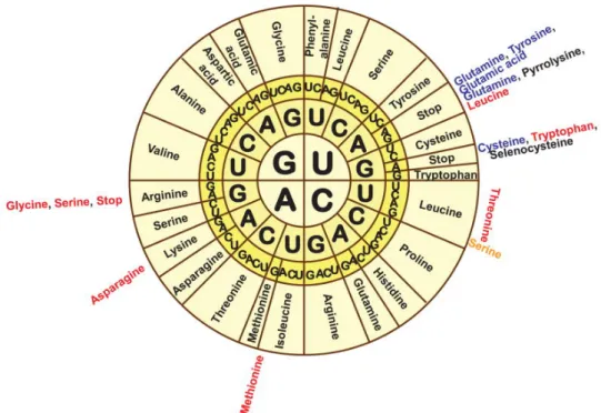
The array of a base sequence defines the sequence of an amino acid which in turn defines the structure of a protein. Proteins are chains that are linked together by amino acids which differ in their length and array. They are synthesized according to their base order in the DNA. One of 20 possible amino acids is encoded by a base triplet (codon). The assignment of the base triplet to its respective amino acid is specified by the genetic code, see Figure 2.2. Some amino acids are encoded by more than one codon.
The protein biosynthese is one of the most important life processes in cells of living organisms. It consists of two subprocesses, the transcription and translation process (see Figure 2.3). During the transcription process the DNA sequence is transcribed into complementary mRNA. In contrast to the double-stranded DNA, the RNA is single-stranded. As the DNA consists of coding and non-coding sequences, theexonsandintrons, the transcribed non-coding sequences are excised from the pre-mRNA (preliminary messengerRNA) while the exons are retained. This process, known assplicing, plays a decisive role in regulating gene expression. However, due the accidental deletion of single exons during the splicing process, mRNA molecules of the same pre-mRNA may differ from one another. The variations resulting from the different composition of the exons in the mRNA might alter the protein structure. Thus, the splicing permits a wide variation of possible nucleotide combinations in the mRNA. These slightly modified proteins are calledisoformes. Although isoformes are encoded by the same gene, they might execute different functions. The structural differences can either prevent the gene from functioning properly or just result in silent mutations, that means meaningless protein variants. Splicing is the reason why the human genome consists of much more proteins than genes. Moreover, allelic differences in mRNA splicing are often associated with genetic disease susceptibility.
Once the mRNA chain is generated, the synthesis of proteins can start. This process, known as translation, is the key process of the protein biosynthesis. The base sequence of the mRNA is translated sequentially into the corresponding amino acid sequence. Amino acids are bonded together by peptide bonds. Two amino acids join together to form dipeptides, more than ten amino acids form polypeptides, and more than 100 amino acids build proteins.
2.2 Affymetrix GeneChip Technology
Microarray technologies belong to the group of high throughput technologies which are used to generate expression data of tens of thousands of genes simultaneously. In the early 1990s, the US company Affymetrix developed the world’s first commercial high-density chip for the analysis of
2.2 Affymetrix GeneChip Technology 7
Figure 2.2:The genetic code: The wheel is read from the inside out with each triplet coding for one
particular amino acid. The sequence AUG encodes the start codon and the sequences UAA, UAG, and UGA encode the stop codons (Lobanov et al., 2010).
gene expression data, the so-called GeneChip. Since then, microarrays are increasingly applied in the field of biomedical research. In practice, two kinds of microarrays are used, one based on cDNA (complementaryDNA) and one based on oligonucleotides. They mainly differ in the way how the base sequences are synthesized on the chip. Affymetrix makes use of the latter method which synthesizes the single-stranded oligonucleotides on the chip base by base by a photolythographic procedure. Technologies using cDNA chips, in contrast, synthesize the complementary DNA sequence as a whole. The latter type of technologies are not part of this work and are therefore not discussed any further. Within this work, only Affymetrix microarray data is used for analysis. Thus, only their GeneChip technology is described in detail.
DNA microarrays allow to capture gene specific sequences in a cell. Conclusions on the phenotype can be drawn by means of sequential composition. Tens of thousands of such RNA transcripts can be captured and measured simultaneously using the Affymetrix’s GeneChip. Depending on the analyzed organism, different GeneChips are used for transcription. The Human Genome U133 Plus 2.0 GeneChip, for example, is used for transcribing the human genome. The chip covers over 50 000 transcripts coding for more than 20 000 genes. Data from rat cells can be analyzed using the Rat Expression Set 230 Array GeneChip or its extended version 230 2.0, each comprising more than 15 000 and 30 000 transcripts and variants from
Figure 2.3:From DNA to protein: The DNA sequence is transcribed into the corresponding RNA sequence by transcribing the base sequence of the gene into its complementary RNA nucleotide sequence. A base triplett encodes for a particular amino acid and the chain of amino acids defines the structure of a protein (oerpub/epubjs-demo book, 2017).
over 10 000 and 13 000 genes, respectively. All those chips consist of hundreds of thousands of microscopically small probe cells, each containing millions of copies of a base sequence artificially synthesized of 25 nucleotides. This oligonucleotide sequence is complementary to the base sequence of the target mRNA. 11-20 of such oligonucleotide probes represent one specific transcript. To detect non-specific hybridizations, and to ensure high accuracy and reproducibility of the data, Affymetrix makes use of a paired design to match and mismatch transcripts (see Figure 2.4). The first probe is referred to as a perfect match (PM) probe and perfectly matches the target sequence, i.e. it is completely complementary to the target mRNA. Each PM is paired with a mismatch probe (MM) that is created by replacing the middle (13th) base by its complement. Thus, at this position it should come to no or a substantially weaker binding. The oligonucleotide probes referring to one probe set differ from one another in terms of their base sequences, such that 11-20 different exon regions of a gene are covered. To avoid spatial effects, the probe pairs of a particular probe set are spread all over the chip.
First of all mRNA is extracted from the tissue of interest. Then it is reverse transcribed into complementary DNA (cDNA). This newly created cDNA serves as template for the amplification of the mRNA. The resulting cRNA molecules are fragmented, labeled with a fluorescent dye and are fixed onto the array such that they can hybridize with their complementary probes on the array. The more the probes on the array coincide with the cRNA molecule, the higher the required temperature to disconnect the match. With a temperature increase non-specific hybridizations can be reduced. It is not uncommon that cRNA fragments hybridize with probes they are not
2.3 Data Preprocessing 9
Figure 2.4:GeneChip expression array design. Structure of a probe set with 16 probe pairs. One
probe pair consists of a perfect-match (PM) and a mismatch (MM) of which each consists
of 21 oligonucleotides. Both sequences are identical except for the 13th base which
is replaced by the corresponding complementary base. The PM probe is completely complementary to the base sequence of the target mRNA, whereas the MM probes serve as control. A probe set is represented by multiple probe pairs (PBworks, 2016).
intended to hybridize. The MM probes serves as controls for measuring background signals. In the case that only sub-sequences of the cRNA are complementary to the probes, less hydrogen bonds are formed during the binding process such that this kind of bindings can be released easier than the intended ones. As soon as the fluorescently stained cRNAs have interacted with their complementary oligonucleotides a light signal is provided. The unbound cRNA fragments are washed out and the hybridization pattern can be read off from the light distribution. A high definition laser scanner scans the intensity of the fluorescent signals which is used as a measure for the quantity of hybridized target RNA. The intensity values are combined into one raw
expression valueper probe set and stored as CEL files (see Figure 2.5 for procedure overview).
2.3 Data Preprocessing
As previously described, multiple probe pairs quantify one probe set which represents a gene. A gene in turn can be encoded by multiple probe sets. The step, in which the scanned data is reduced from probe level to gene level, is referred to as pre-processing. There exist a number of pre-processing algorithms which all summarize single probe set intensities to one representative expression value. Robust Multiarray Analysis (RMA) proposed by Irizarry et al. (2003a) is one of the most commonly used pre-processing algorithms for Affymetrix microarray data. In a three-stage process the data is background-corrected, normalized and finally summerized to
Figure 2.5:Affymetrix microarrays: Photolithographic synthesis of oligonucleotides on microarrays. A chip consists of hundreds of thousands of microscopically small probe cells. Each cell contains millions of copies of oligonucleotide sequences which serve as template for the hybridization of the probes with their fluorescently labeled mRNA targets. The fluorescent signals are read by a high definition laser scanner and are combined into one raw expression value per probe set (Affymetrix, 2017).
one value. However, the simultaneous analysis of data requires the simultaneous pre-processing of the respective microarrays. This interdependency of multiple microarrays has one obvious disadvantage: The inclusion of new microarrays implicate the re-pre-processing of the original data set which has to be pre-processed together with the new microarrays, and this process changes again the gene expressions of the original data. Thus, separate pre-processed data sets are not comparable. To ensure the comparability of results across different arrays wihtout changing the expression values of previously pre-processed microarrays Harbron et al. (2007) propose an extended version of the RMA algorithm, which they refer to as RMA+ algorithm. The idea is based on the calculation of reference parameters estimated from a reference set of microarrays which are stored and used for the normalization process of future microarrays. In this manner, the key properties of the RMA algorithm are maintained and new microarrays can be normalized in addition to the already pre-processed ones without re-estimating the reference parameters. This extension of the RMA algorithm allows the joint analysis of arrays analyzed in
2.3 Data Preprocessing 11
different batches. The RMA+ algorithm is being implemented in the packageRefPlusfor the open source statistical software R (Chang et al., 2016).
The RMA+ algorithm makes use of theExtrapolation Strategywhich splits the data into two sets of microarrays: One set is used as the reference set and the other one as the future set. The reference parameters are estimated from the reference set and are applied to the future set. They are obtained from fitting an RMA model to the reference set. This is accomplished by the aforementioned three-step procedure. Background correction is performed on each array individually and is therefore not discussed here. The reader is referred to Irizarry et al. (2003b) for a detailed explanation of the background correction procedure. After the intensity values have been background-corrected, a normalization step is required to achieve comparability across all arrays. As the slightest differences in the test execution, be it in the target preparation or in the hybridization procedure, might lead to a wide dispersion of the intensity values between arrays, RMA uses quantile normalization to normalize the probe intensities to a common set of quantiles, such that the intensities of all arrays have the same distribution. In the last step, the background-corrected and normalized probe set intensities are summarized to one expression value.
Letidenote the microarray andjthe probe of a probe set, then thelog2background-corrected and normalized intensityNij of probej on arrayiis given by:
Nij =Pj+Ii+ij, (2.1)
whereP is the effect of the jth probe, I is the expression of the probe set on array i and ij
indicates the error term. The expression value is estimated for each probe set separately by using Tukey’s median polish which is an algorithm for calculating a robust average over all probes and arrays.
The probe set intensities of the reference set are stored together with their estimated quantiles and probe effects. The future microarrays undergo the same three-step procedure as the reference set: Background-correction, quantile normalization and aggregation to one expression value. But this time the microarrays are normalized to the reference quantiles. Assuming that the probe effects of the future set equal those of the reference set, the probe set intensityI˜f of a future
arrayf is estimated from the model in (2.1) and given by
˜
whereNf jindicates the background-corrected and normalized intensity of probejon arrayf
andPj represents the effect of thejthreference probe.
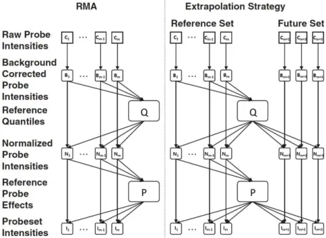
Figure 2.6 compares the RMA algorithm with its extended version, the RMA+ algorithm.
Figure 2.6:Illustration of the RMA and RMA+ algorithm. Both algorithms uses background
cor-rection, quantile normalization and a linear model fit to the normalized data to obtain an intensity value for each probe set. In contrast to the RMA algorithm which uses the information of the complete microarray set the RMA+ algorithm makes use of the extrapolation strategy which splits the data into two sets of microarrays, the reference-and the future set. The reference set is used for the estimation of the reference parameters which are stored and used for the future set. The reference parameter are obtained from fitting a RMA model to the reference set. (Slightly modified version of a figure provided by Harbron et al. (2007)).
2.4 Data sets 13
2.4 Data sets
Within the scope of this work, several data sets were used for analysis. All analyses were performed on the basis of Affymetrix gene expression data. For the normalization of the arrays, the Robust Multi-Array Average (RMA+) algorithm was applied. As reference, different normalization parameters were used which depended on the used model organism. The respective parameters were obtained from fitting a RMA model to previously analyzed data of the same GeneChip. The estimated parameters were stored and applied to the currently analyzed arrays.
After normalization, the difference in gene expression between treated- and corresponding untreated samples was calculated for each test condition separately. The subtraction procedure was based on averaged replicate values. As gene expression data is measured on alog2-scale, the difference between logarithmized average values corresponds to the logarithmized fold change FCi of genei: log (FCi) = log ¯ xExpi ¯ xCtrl i ! = log v u u t n Y j=1 xExpij −log v u u t n Y j=1 xCtrl ij = log xExpi1 ·. . .·xExpin 1 n −logh xCtrli1 ·. . .·xCtrlin 1 ni = 1 n " n X j=1 log xExpij # − 1 n " n X j=1 log xCtrlij # ,
wherexExpij denotes the gene expression for genei,i= 1, . . . , nPS, and arrayj,j = 1, . . . , n,
andxCtrl
ij the corresponding control value. The termsx¯ Exp
i andx¯Ctrli indicate the geometric mean
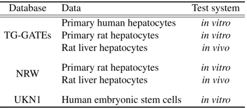
of the exposed samples and the controls, respectively. The fold change is used as a measure for the exposure-related effect of a compound. All analyses base on the fold change values of a gene. However, the termgene expressionis used in that context. Table 2.1 provides an overview of the data sets used for analysis.
2.4.1 TG-GATEs database
TGP (TheToxicogenomicsProject) is a project funded by both the Japanese government and the private sector. The National Institute of Biomedical Innovation (NIBIO, 2017), the National
Institute of Health Sciences (NIHS, 2017) as well as the pharmaceutical industry contributed to its establishment. Between 2002 and 2006, gene array data was generated within the project testing ≈150 compounds, including hepatotoxic and non-hepatotoxic ones, in primary human and rat hepatocytes as well as rat liver and kidney cellsin vivo. That data was used to generate a large-scale toxicogenomic database. The TG-GATEs (ToxicoGenomics Project-GenomicsAssisted
ToxicityEvaluationSystem) database was then finally created by integrating further options into
the existing database system. The extended database offered possibilities of performing targeted analyses for the prediction of toxicity of the test compounds. TGP2 (The Toxicogenomics Informatics Project 2) was a follow-up project of TGP that was initiated in 2007 by the same founder. In the period from 2007 to 2011 30 safety biomarkes were detected within the framework of this project by using the TG-GATEs database. The new data gained by TGP2 was included into TG-GATEs. Open TG-GATEs is a publicly available database for the use of non-profit purposes. The raw microarray data (CEL files) for all analyzed compounds and conditions can be downloaded from the Open TG-GATEs website (http://toxico.nibiohn.go.jp/english/index.html). The portal has been developed to give scientists the opportunity to use the research results of TGP and TGP2. The user is free to use the data for both scientific and private purposes, including the publication of results and the disclosure of the information to third parties. The database compiles Affymetrix HG U133 Plus 2.0 gene expression microarray data on 170 compounds. The search for data is enabled via compound name or pathological findings by organ. Access to phenotype data is provided as well. The documents contain information about the experimental setup, the histopathological findings and the research results of the TGP project which are supplied as PDF file and can be viewed directly or downloaded from the homepage. Currently, the documents are only available in Japanese (NIBIOHN, 2017).
Table 2.1:Overview of the data sets used in the analyses.
Database Data Test system
Primary human hepatocytes in vitro
Primary rat hepatocytes in vitro
TG-GATEs
Rat liver hepatocytes in vivo
Primary rat hepatocytes in vitro
NRW
Rat liver hepatocytes in vivo
2.4 Data sets 15
Primary human hepatocytes
The primary human hepatocytes were treated with different test compounds using three con-centrations (Low, Middle, High) and three incubation periods (2h, 8h, and 24h). For cytotoxic compounds the highest tested concentration was chosen such that it represented approximately the EC10(the concentration that produces 10%reduction of the maximal effect). Each
concen-tration was assessed using two replicate experiments. Table 2.2 provides an overview of the experimental design. A subset of compounds was tested under all conditions (n=52), while most of the compounds were tested only under some of the conditions. The compounds were tested either for only one or two exposure periods, or with only two concentrations, as shown in Table B.1 in the Appendix. Experiments without replication, as well as experiments including cytokines and LPS (lipopolysaccharide), were excluded from the analyses. Cytokines are proteins involved in the regulation of proliferation and differentiation processes in cells. Seven of the tested compounds were cytokines and due to their molecular functionality excluded. Table 2.2 shows the number of compounds tested under the indicated condition with and without cytokines in brackets.
Table 2.2:Matrix of the compounds tested in primary human hepatocytes. The table provides the
numbers of compounds tested under the indicated condition, for each combination of concentration and exposure period, before and after (in brackets) excluding cytokines and LPS (lipopolysaccharide) from the analyses.
2h 8h 24h Overlap
Low 53 (48) 82 (75) 81 (75) 52 (48) Middle 53 (48) 153 (146) 157 (151) 52 (48) High 53 (48) 153 (146) 153 (148) 52 (48) Overlap 53 (48) 82 (75) 77 (72) 52 (48)
Primary rat hepatocytes
The cultured rat hepatocytes were tested in duplicates with the indicated compounds using a low, middle and high concentration for the incubation periods 2h, 8h, 24h. For a detailed overview of the data the reader is referred to Table B.2 in the Appendix. The highest tested concentration was again chosen close to cytotoxic levels. Table 2.3 shows the number of compounds tested at the indicated concentration and time sets. The same exclusion criteria as those for the human hepatocytes were applied to the data from the rat model, for both thein vitroand in vivotest system.
Table 2.3:Matrix of the compounds tested in primary rat hepatocytes. The table provides the numbers of compounds tested under the indicated conditions for each combination of concentration and exposure period, before and after (in brackets) excluding cytokines and LPS (lipopolysaccharide) from the analyses.
2h 8h 24h Overlap
Low 140 (138) 140 (138) 145 (143) 140 (138) Middle 140 (138) 140 (138) 140 (138) 140 (138) High 138 (137) 139 (138) 138 (137) 138 (137) Overlap 138 (138) 139 (137) 138 (138) 52 (48)
Rat liver hepatocytes
Rat liver samples were treated with the compounds listed in Tables B.3 and B.4 which are given in the Appendix. Each compound was tested at three concentrations (Low, Middle, High) and sacrificed at different time periods after exposure. This time eight incubation times (3h, 6h, 9h, 24h, 4 days, 8 days, 15 days, 29 days) were investigated, using three replicates in each experiment. Table 2.4 summarizes the compounds with available data with respect to the indicated test condition.
Table 2.4:Matrix of the compounds tested in rat liver cells. The tables provide the numbers of
compounds tested under the indicated conditions for each combination of concentra-tion and exposure period, before and after (in brackets) excluding cytokines and LPS (lipopolysaccharide) from the analyses.
3h 6h 9h 24h Overlap
Low 153 (151) 153 (151) 153 (151) 157 (155) 153 (151) Middle 152 (150) 153 (151) 153 (151) 157 (155) 152 (150) High 151 (149) 151 (149) 151 (149) 153 (151) 150 (148) Overlap 150 (148) 150 (148) 150 (148) 152 (150) 149 (147) 4 days 8 days 15 days 29 days Overlap Low 141 (141) 141 (141) 141 (141) 141 (141) 141 (141) Middle 141 (141) 141 (141) 141 (141) 141 (141) 141 (141) High 143 (143) 143 (143) 139 (139) 127 (127) 127 (127) Overlap 141 (141) 141 (141) 138 (138) 126 (126) 126 (126)
The reader is referred to the Tables B.1-B.4 in the Appendix which provide a detailed compound-specific summary for the three model organisms. The tables give full and abbrevi-ated compound names as well as the concentration in µM (µg/mL, µg/kg) and the number of
2.4 Data sets 17
independent replicates of gene array data available after incubation with a low, middle and high concentration for the indicated exposure period.
2.4.2 UKN1 test system
Embryonic stem cell (ESC)-based systems have been developed to recapitulate in vitro the differentiation of stem cells into neuronal cells. Stem cells have the property of pluripotency, i.e. the ability to differentiate into all types of cells. During the differentiation process different mechanisms such as cell proliferation, migration and apoptosis are induced. Cultures of differen-tiating human embryonic stem cells (hESC) offer the opportunity to observe, study and control the early steps of human development. External stimulus influences, such as drug exposure, can interfere with early developmental stages. In that context, different human ESC (hESC)-basedin
vitrosystems have been developed to recapitulate the different phases of early tissue specification
and neural development. The UKN1 test system is one of them and was developed to model the stage of differentiation of neuroepithelial precursor cells (NEP) from hESC. Figure 2.7 visualizes the test system’s treatment protocol. In that system the cells were exposed to the test compounds within 6 days. In the present study two compounds, valproic acid (VPA) and methylmercury (MeHg), were tested to detect chemically-induced gene expression alterations. VPA is used as an anti-epileptic drug and known to cause neural tube defects, just as MeHg. Earlier analyses have shown that exposure-related effects strongly depend on the concentration of the test compound. Therefore, the compounds were tested with different concentrations covering non-toxic to toxic concentrations. The highest concentration was chosen according to a benchmark concentration representing the EC10. For more details on the test systems the reader is referred to Krug et al.
(2013).
VPA chronic concentration study
The VPA concentration study was conducted to investigate the development of human embryonic stem cells (hESC) to neuroectoderm. The cells were treatedin vitrowith valproic acid (VPA) using eight different concentrations (25-1000 µM). Each concentration was assessed using three replicate experiments (see Table 2.5). The compound was exposed to the cells during the entire differentiation process. In addition, six untreated measurements were available. Replicates of controls were averaged before subtracting from corresponding exposed samples (paired design). The study was carried out within the framework of the European Commission-funded research
consortium (ESNATS) which targets the prediction of toxicity of drug candidates for the use of embryonic stem cell-based novel alternative tests.
Figure 2.7:Overview of the UKN1 test system’s treatment protocol. The test system recapitulates
the differentiation process of human embryonic stem cells (hESC) to neuroepithelial precursor cells (NEP). The cells were treated with valproic acid (VPA). The bars below the test system provide information on replating, medium change, toxicant exposure and day of array analysis, as indicated in the legend to the right (Krug et al., 2013).
Table 2.5:Overview of the number of replicates used in the VPA chronic concentration study.
Concentration in µM
0 25 150 350 450 550 650 800 1000
6 3 3 3 3 3 3 3 3
2.4.3 NRW database
The NRW data set comprises 30 compounds that have been tested in rats in vivo (Ellinger-Ziegelbauer et al., 2008) and 29 compounds that have been tested in cultivated rat hepatocytes (Schug, 2011). With the exception of one compound (Phenobarbital) that was only exposed to rat cellsin vivo, the other 29 test compounds were the same. Male Wistar rats were used as model organism for both test systems.
2.4 Data sets 19
In vivo rat cell culture
Primary rat hepatocytes within vivorat liver data were treated with each compound in 3 replicates and sacrificed after 6h, 12h, 24h, 48h, 3 days, 7 days and 14 days after exposure. Incubation peri-ods of 6h, 12h and 48h were not considered any further as only one compound (Acetaminophen) was tested for these time periods. Table B.5 in the Appendix contains an overview of the number of replicates used in thein vivo experiments. The rat liver cells were obtained from five animals treated daily with each compound. The treatment of animals was performed in different experimental series. Therefore, ’experimental series’- and ’exposure period’-matched controls were subtracted from the corresponding treated samples. The concentrations used for the individual compounds during the entire incubation period are indicated in Table B.5 as well. For transcriptional analysis therae230aarray was used which comprises 15 923 probe sets, corresponding to approximately 10 045 annotated genes. As no reference parameters are provided for this chip, the arrays of the treated samples were normalized to the complete set of control arrays. The study was originally conducted to predict the toxicity class of unknown compounds. A classifier that separated genotoxic from non-genotoxic carcinogens was built from a set of training compounds (n=13) and applied to an independent set of validation compounds (n=16). The training and validation sets together form the database for thein vivoanalyses. The classification into the annotated categories is given in the Appendix in Table B.5.
In vitro rat cell culture
Cultured rat hepatocytes were also tested with three replicates using three concentrations (Low, Middle and High) and one incubation period (24h). The highest concentration represents the EC20. Similar to thein vivoexperiments, not all concentration- and time sets are complete. Some
of the compounds were tested only for two conditions as shown in Table B.6 in the Appendix. The experiments were organised in 6-well-dishes. Per concentration, 3-wells were incubated with the test compound and 3-wells were used as controls. According to that test design, the controls were 6-well dish- matched subtracted from the corresponding exposed samples. Transcriptional analysis was performed by using the rat2302-GeneChip 31 099 probe sets encoding 13 685 genes. For comparability reasons, the analyses was restricted to those transcripts that have been measured on the rae230a-GeneChip which was used for the in vivoexperiments. For the normalization of the entire set of expression arrays the RMA+ algorithm was used which provided reference parameters for future data sets, such as the TG-GATEs rat data sets.
This chapter provides an overview of the statistical methods used for data analysis in this thesis. First, multivariate methods for pattern recognition are introduced. The basic principle of principal component analysis is explained and the heatmap is introduced as a visualization method for high-dimensional data. In Section 3.3 the Limma t-test, which is used for the analysis of high-dimensional gene expression data, is outlined. In the context of dose-finding studies, several indices for the description of concentration-dependent progressions are presented (Section 3.4). Section 3.5 deals with the theory of dose-response models. Within this section, the four-parameter-log-logistic model (4pLL) together with its estimate for the Absolute Lowest Effective Concentration (ALEC) is presented. Moreover, it is elucidated how to construct confidence intervals for the effect level (response) and to how calculate the lowest effective concentration (LEC) by means of hypothesis testing.
3.1 Principal component analysis
Principal component analysis (PCA) is a multivariate procedure for the detection of structures in large data sets. The method targets to reduce the dimensionality of data by projecting the data into a lower-dimensional space while aiming for preservation of information. The approach implies the construction of uncorrelated linear combinations representing the principal components which are sorted according to the proportion of their explained variance in descending order. Thereby the total variance serves as a measure for the information content. LetX> = [X1, . . . , Xp]be
ap-dimensional vector of ann×pdata matrix withnobservations andpvariables. The idea is to transform the coordinate system that is spanned by the random variablesX1, . . . , Xp by
rotation into a new coordinate system, the vector subspaceRk(k < p). The objective is to find a set of linearly uncorrelated components that are orthogonal to each other and sorted in order of their magnitude, i.e. such that the first principal component explains most of the data variability, the second component contains the next most information and the last components provide the
3.1 Principal component analysis 21
slightest information. If a sufficiently large proportion of total variance is covered by the first
kprincipal components, they prove to be sufficient to reproduce the data variability with little loss of information. The remainingp−kcomponents make only an insignificant contribution to the overall variance and can therefore be neglected. The coordinate system spanned by the
k principal components allows a simplified depiction of the data structure or their covariance matrix, respectively, in ak-dimensional space.
Consider now the vector X> = [X1, . . . , Xp] with covariance matrix Σ and eigenvalues λ1 ≥. . .≥λp >0. Further, letA= (a1, . . . , an)be an orthogonalp×pmatrix, i.e.A>A=Ip.
Then the principal componentsY1, . . . , Yp are obtained by the transformation of X> → Y>
given by Y1 =a1>X =a11X1+a12X2+. . .+a1pXp Y2 =a2>X =a21X1+a22X2+. . .+a2pXp (3.1) .. . ... Yp =ap>X =ap1X1+ap2X2+. . .+appXp,
wherea1> = (a11, . . . , a1p), . . . ,ap> = (ap1, . . . , app)are the vectors of weights. SinceAis
orthogonal the transformation corresponds to a rotation of the n points in thep-dimensional space.
The first principal component minimizes the sum of the Euclidean distances between the projected data points and the original ones and maximizes the variance of the projections. Hence, the variance of Y1 = a>1X must be maximized subject to a>1a1 = 1. A method for the
optimization of a function subject to a constraint is the method of Lagrange multipliers. The functionLto be maximized is given by
L(a1, λ1) =a>1Σa1 | {z } fct. to max. −λ1(a>1a1−1) | {z } constraint , (3.2)
whereλ1 ∈Rdenotes a Lagrange multiplier. The function in (3.2) is differentiated with respect toa1 andλ1 and subsequently set equal to zero:
1)∂λ∂L 1 = 1−a1 >a 1 2)∂∂La1 = 2Σa1−2λ1a1 ! = 0. (3.3)
The system of equations in (3.3) shows that the vector a1 has to satisfy a>1a1 = 1 and
Σa1 = λ1a1. The second term equals an eigenequation with the Langrange multiplier as
eigenvalue meaning that a1 is the normalized eigenvalue of the covariance matrix Σ with
eigenvalue λ1. Hereafter, let ei denote the eigenvector to eigenvalue i. The first principal
component is obtained by the projection ofX> ontoe1which is the eigenvector corresponding
to the largest eigenvalueλ1. The remaining principal components are constructed recursively
to the preceding ones such that the projections onto thekthprincipal component have maximal variance and are orthogonal to the firstk−1principal components, i.e.ai>ak = 0,1≤i < k.
Thus, the second principal component has to maximize
L(a1,a2, µ, λ2) =a2>Σa2 | {z } fct. to max. −µa2>a1 | {z } constraint −λ2(a2>a2−1) | {z } constraint , (3.4)
whereµ∈Randλ2 ∈Rindicate the multipliers. Differentiating function (3.4) with respect to all parameters and setting the partial derivatives equal to zero, delivers the second most important linear combinatione>2X which maximizesVar e>2X
subject to the required constraints. The remaining components are constructed analogously, i.e. theithlinear combination maximizes
Var e>i X
with respect to both constraints,e>i ei = 1andCov e>i X, e>kX
= 0fork < i. By induction, it can be shown that the first k principal components correspond to the first k
eigenvalues.
Replacing the coefficients ai, i = 1, . . . , p from equation (3.1) with the normalized and
orthogonal eigenvectorseileads to the besti-dimensional approximations
Yi =ei>X =ei1X1+ei2X2+. . .+eipXp, i= 1, . . . , p
with the following properties
i) Var (Yi) =e>i Σei =λie>i ei =λi, i= 1, . . . , p
ii) Cov (Yi, Yk) = ei>Σek = 0, i, k = 1, . . . , p,
subject to the constrainte>i ei= 1.
The covariance matrixΣcan be rewritten asΣ=UΛU> by means of Spectral Decomposi-tion (SD), whereΛis a diagonal matrix whose diagonal entries are the eigenvaluesλ1, . . . , λp
3.1 Principal component analysis 23
detailed description of the theory of SD, the reader is referred to Johnson and Wichern (1998). The matrixU has the property:U U> =U>U =I.
The vectorse1, . . . ,epprovide an orthogonal basis, i.e.U corresponds to the vector subspace
into whichX> is projected: Y> =X>U. As a rotation is obtained by the multiplication of a scalar with a orthogonal matrix, the transformationX> → Y> corresponds to the rotated coordinate system.
The vector e>i = (ei1, . . . , eik, . . . , eip) can be interpreted as the score vector of the
prin-cipal component whose components eik, i, k = 1, . . . , p, indicate how good the kth variable
is approximated by the ith principal component. The firstk principal components explain a proportion of
Pk
i=1λi
Pp
j=1λj
of the total variance.
The equation in (3.6) for the correlation ofYi und Xk can be justified by choosing a>k = [0, . . . ,0,1,0, . . . ,0] | {z } kthposition such that Xk=a>kX, Cov (Xk, Yi) = Cov a>kX,e>i X =a>kΣei =a>kλiei=λieik. (3.5)
The variance ofYi andXksatisfy: Var (Yi) =λiandVar (Xk) =σk, respectively. It follows
ρYi,Xk = Cov (Yi, Xk) p Var (Yi) p Var (Xk) = √λieik λi √ σk = eik √ λi √ σk , i, k = 1, . . . , p. (3.6)
If the variables are not measured in the same scale unit, it is recommended to perform the PCA on the basis of the correlation matrix rather than the covariance matrix, since the variables are not comparable with each other. With respect to microarray analysis, standardization of the data is not required as the variables representing the expression values are measured on the same scale (log2). Usually, PCA is used as a prestep in a comprehensive analysis to obtain a first overview of the data. Often, the first two components are sufficient to reveal features such as batches or outliers.
3.2 Heatmap
Heatmaps are a commonly used graphical method for the visualization of gene expression data where rows and columns represent the genes of interest with respect to the analyzed arrays. A heatmap compresses large amounts of information into a compact display area and, hence, allows the visual detection of coherent patterns. A matrix containing the expression values of genes is color encoded according to the values’ order of magnitude and displayed as color image. Usually, heat colors are used for illustrating the data which is the reason for the name of the heatmap. Many software systems such as the statistical softwareRuse the heat colors as default. Generally, different color schemes can be used to visualize the colormap. In the context of gene expression data, it is useful to map the range of values to colors ranging from blue to red with blue colors indicating low expression levels and red colors high expression values.
Coherent patterns of color are generated by hierarchical clustering. The rows and columns of the data matrix are permuted such that objects with similar expression profiles are clustered together. Cluster relationships are indicated by dendrograms generated for both axes. The resulting patterns indicate functional relationships between the arrays and genes (Wilkinson and Friendly, 2009). Heatmaps can be produced by using theRstandard packagestats(R Core Team, 2015). It is up to the user to decide which agglomeration rule and metric should be used for the cluster analysis. Thecomplete linkage methodis used by default to reorder the dendrograms. Alternatively, both dendrograms can be reordered by a prescribed vector of values or be completely omitted. By default, the Euclidean distance is used as distance measure for the calculation of pairwise distances. Thegplotpackage implements an extended version of the standardRfunction which offers a number of additional features such as acolor keyillustrating the range of values together with their distribution, or a side bar that may be used to classify the objects with respect to any characteristics (Warnes et al., 2015).
Figure 3.1 shows an example for a heatmap, where rows represent genes and columns indicate samples. For illustration purposes, gene expression data of human embryonic stem cells (hESCs) after VPA (valproic acid) exposure was used. Originally, the cells were treated with eight different concentrations (25-1000 µM withn=30) using three replicates (for more details on the study see Section 2.4). For generating the exemplary heatmap only a subset of the measured concentrations was used (150 µM, 550 µM, 800 µM, 1000 µM withn=12 samples). The absolute gene expression levels (log2-scaling) of the ten transcripts with highest variance across the
3.2 Heatmap 25
12 samples were color-coded for display. The samples have been classified with respect to concentration level and replicate number. Up- and downregulation is indicated by blue and red coloring. Replicate Concentration 1 3 2 4 5 6 7 9 8 10 12 11 MAB21L2 RSPO2 ARX HAPLN1 MUC15 MUC15 SLC40A1 HAPLN1 SIX1 CR1L 4 6 8 10 Value Color Key Replicate 1 2 3 Concentration 150µM 550µM 800µM 1000µM
Figure 3.1:Example of a heatmap. Each row represents a gene, while each column stands for a
sample. Red color indicates up- and blue color downregulated genes as indicated by the color key in the upper left. The rows and columns are reordered according to their respective dendrograms which are generated by hierarchical clustering. The samples have been classified according to concentration level and replicate number which are indicated by the column side bar and the legends in the upper right and upper left.
3.3 Limma: Linear Models for Microarray Data
Limma is anR/Bioconducterpackage which is used for the analysis of gene expression data (Ritchie et al., 2015). TheLimmat-test is a moderatedt-test for detecting gene expression changes which are associated with a particular treatment condition. The simplet-test is altered in the sense that the information of the complete set of genes is used in the estimation of the gene-wise variances in place of the ordinary variances. The basic idea ofLimmais to shrink the gene-wise residual sample variances towards a common value by an empirical Bayes approach. The effect of sharing information has, especially in case of small sample sizes, the advantage of more accurate estimators and therefore less unbiased test results.
Consider a microarray experiment withn arrays where yg> = (yg1, . . . , ygn)denotes the
response vector which contains the expression values of geneg. This means that the response of geneg corresponds to thegthrow of the expression matrix. LetX be the design matrix with
rows representing the arrays andαg the vector of coefficients. LetC denote the contrast matrix
whose rows correspond to the coefficients and whose columns contain the contrasts. In case that only one contrast is of interest, a contrast vector is defined. The contrast matrix allows to adjust for covariates, batch- or interaction effects. In terms of a linear model
E(yg) =Xαg.
The variance of the response vectorygis given by
var(yg) = Wgσg2,
where Wg is a positive definite weight matrix which allows the incorporation of unequal
variances for more accurate test results, and σg2 indicates for gene g the residual variance of the model with dg residual degrees of freedom. Samples can be individually weighted
according to their reliability (Smyth, 2005). The contrasts of interest are defined by βg =
C>αg. Given the expression- and design matrix the lmFit() function fits a linear model
to gene g. The same model is applied to the other genes of the microarray experiment. The coefficientcomponent contains the estimated coefficients forαg. Given the fitted model,
thecontrast.fit()function estimates the coefficients and standard errors forβg. Unlike
3.3 Limma: Linear Models for Microarray Data 27
dependent. That means that the number of contrasts does not necessarily have to be the same as that of the coefficients. It is quite possible that the contrasts correspond to a subset of the original coefficients. As the coefficients themselves are usually of no further interest, but certain contrasts of them, they are re-calculated together with their standard deviations and their covariance matrix into the corresponding contrast objects. In the special case that the design matrix consists of a singlen-dimensional column of onesX> = (1, . . .1), theLimmat-test equals a simplet-test but adjusted for the gene-wise variance estimator which comprises both, the information of the gene alone and the pooled one of all genes. The contrast matrix is redundant in that case and can be omitted. The simplest experimental design is a microarray experiment with two treatment groups comparing experiment and controlRNA. If the entries in the gene expression matrix correspond to thelog2-fold changes, i.e. the differences in gene expression between experiment and control, the coefficient vectorαgconsists only of one elementαg. The coefficient estimator
corresponds to the meanlog2-fold changes of thegthgene. In that special case, the coefficientαg
corresponds to the contrast of interest, namely the treatment effect.
As mentioned above, the coefficient estimatorαbg, the estimators2gof the residual varianceσg2
and the estimated covariance matrix ofαbg:varc( ˆαg) =Wgs 2
g are re-calculated in terms of the
contrastsβˆg =C>αbg. Given the contrast matrixCand the weight matrixWg, the covariance
matrix ofβg is estimated by c var( ˆβg) =C>WgC | {z } Ug s2g.
Unlike the responsesyg, for which no distributional assumptions are made, the contrast estimators are assumed to be at least approximately normally distributed with mean βg and covariance matrixC>WgCσg2. LetUg = C>WgC be the matrix whose diagonal entries correspond to
the unscaled variances ofβˆg, then thejthdiagonal entryugj denotes the variance ofβˆgj and the
ordinaryt-statistics for thejth contrast is given by
tgj = ˆ βgj sg √ ugj , (3.7)
which ist-distributed withdg degrees of freedom.
Thus, thejth component of the estimated contrast vectorβˆg satisfies
ˆ
βgj
and s2gσg2 ∼ σ2 g dg χ2dg, wheres2
g is approximatelyχ2-distributed withdg degrees of freedom.
The empirical Bayes approach uses a hierarchical model to estimate the posterior residual variances. The basic idea is to incorporate the common information provided by all genes together into the gene-wise sample variance. The residual varianceσ2g is assumed to be a priori inverseχ2-distributed withd
0 degrees of freedom 1 σ2 g ∼ 1 d0s20 χ2d0, (3.8) wheres2
0 is a further hyperparameter which is estimated from the data, similar tod0. It can be
shown that theχ2-distribution in (3.8) can be rewritten as gamma distribution:
d0s20 σ2 g ∼χ2d0 ⇒ 1 σ2 g ∼Γ k= d0 2 , θ= 2 d0s20 .
The estimators for both parameters,s2
0andd0, are obtained from the observed sample variances s2g. Hence, the inverse posterior estimator for the residual variance ˜s1
g corresponds to the mean of the gamma distribution which is the a posteriori distribution of σ12
g (Rempel, 2015): 1 σ2 g (s20, d0, s2g)∼Γ k = d0+dg 2 , θ= 2 d0s20+dgs2g . It follows 1 ˜ s2 g =E 1 σ2 g s20, d0, s2g = d0+dg d0s20+dgs2g ⇒s˜2g = d0s 2 0+dgs2g d0+dg .
For more details the reader is referred to Rempel (2015).
Substituting the prior standard deviationsg in the ordinaryt-statistic, given in (3.7), by the
posterior standard deviations˜g, results in the moderatedt-statistic
˜ tgj = ˆ βgj ˜ sg √ ugj ,
which ist-distributed with(d0+dg)degrees of freedom under the null hypothesisH0 : βgj = 0.
3.4 Statistics for concentration-dependent analyses 29
the other genes to adjust the individual genes in terms of the global variance. In case ofd0 = 0,
˜
tgj =tgjholds (Ritchie et al., 2015).
3.4 Statistics for concentration-dependent analyses
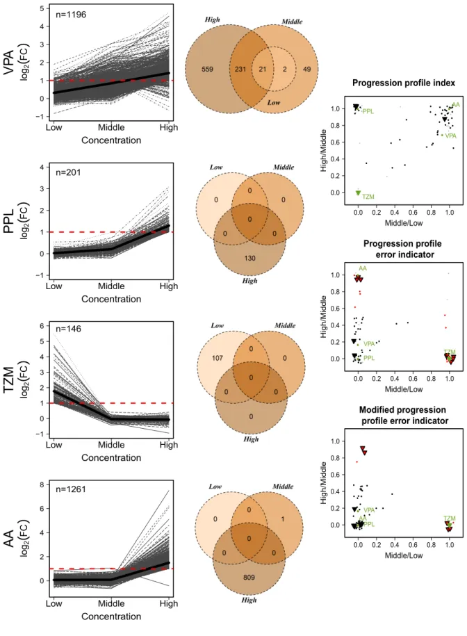
In concentration-dependent gene expression studies a convincing concentration progression is a criterion for data quality. Genes that are deregulated by a compound at a certain tested concentration are usually also deregulated at the next higher concentration. Therefore, genes with a deviating expression profile, i.e. genes with a non-monotonous concentration progression, may be indicative of low-data quality and, hence, should be treated with caution. In order to improve the data reliability, Grinberg et al. (2014) has introduced two indices for the progression analysis of gene alterations over increasing concentration levels, theprogression profile index
and the progression profile error indicator. Both statistics return exclusivity indices for the comparison of adjacent concentrations. They are calculated for each compound and incubation time point separately. Mathematically, the indices are defined as the probability of being not deregulated at a certain concentration level subject to the condition of being deregulated at an other concentration level.
Let C1 andC2 denote two concentration levels andGDiffC1 and G
Diff
C2 the events of being
dif-ferentially expressed at C1 and C2. The complement GDiffC1 indicates the event of being not
differentially expressed atC1. The conditional probability ofGDiffC1 givenG
Diff
C2 is then defined as
the ratio of the probability of the intersection of the eventsGDiff
C1 andG
Diff
C2 , and the probability of
the eventGDiff
C2 : P GDiff C1 |G Diff C2 = PGDiff C1 ∩G Diff C2 P GDiff C2 . (3.9)
This quantity is estimated by replacing the events with the corresponding relative proportions of genes that are deregulated.
3.4.1 Progression profile index
The progression profile index is defined as the ratio of two proportions, the proportion of genes that are deregulated exclusively at the higher concentrationC2, and the proportion of genes that
are deregulated in total at C2. In formula in (3.9) this corresponds to the situationC1 < C2.
concentration, whereas values close to one indicate many additional genes deregulated at the higher concentration.
3.4.2 Progression profile error indicator
The progression profile error indicator is defined vice versa to the progression profile index, namely as the ratio of the proportion of genes that are deregulated exclusively at the lower concentration, and the proportion of genes that are deregulated in total at the lower concentration. In terms of formula (3.9), it holds C1 > C2. Values close to one indicate that a high fraction
of genes are deregulated exclusively at a lower but not at the respective higher concentration. Values close to zero indicate the revers case. Compounds with values above 0.5 are considered as indicative of an implausible concentration progression.
3.4.3 Modified progression profile error indicator
The modified progression profile error indicator is an adjustment of the progression profile error indicator and has been introduced for the case that only a few genes are altered in total. As a certain amount of false positive genes is to be expected, a tolerance limit, i.e. a minimum amount of differentially expressed genes, should be set before including the respective genes in the calculations of the progression profile error indicator. Therefore the number of genes deregulated in total is incorporated in the calculation of that index. The progression profile error indicator is altered in the sense if the value of the index is larger than 0.5 and the number of genes deregulated at the respective lower concentration is below 20, the value of the index is set to zero. The interpretation of the modified index is the same as for the progression profile error indicator.
3.4.4 Selection value
To systematically analyze stereotypic versus compound-specific gene expression responses, the selection value principle has been introduced in Grinberg et al. (2014). A stereotypic response means that an expression alteration is induced by many compounds, while a specific expression response is induced by individual compounds or small numbers of compounds. For a gene, the selection value determines the number of compounds that induces a change in its expression. Compounds are ranked gene-wise in order of magnitude, in case of upregulated genes compounds are ranked from high to low fold changes and in case of downregulated genes from low to high
3.4 Statistics for concentration-dependent analyses 31
values. The selection valuexfor a gene (Svx) defines the rank of the compound, indicating that the gene is induced by at leastxcompounds. The threshold for the critical change is pre-specified. In case of small replicate numbers, it is recommended to consider higher thresholds to keep the number of false positive genes as low as possible. The probability of false positive alerts decreases with increasing fold change. The higher the selection value the less compound-specific is the response. For a given fold change the so-called Sv 20 genes refer to those genes which respond to at least 20 compounds reflecting a stereotypical response. By contrast, a compound-specific response is here specified by Sv 3 genes, i.e. genes which are deregulated by at least three compounds. Note, that genes of higher selection values always overlap with genes of lower selection values, i.e. Sv 20 genes are a subset of Sv 3 genes.
Based on the selection value concept a consensus Svxsignature of genes comprises the Svx
gene lists of all individual test conditions. That means, the consensus Svxlist includes all those genes that show for at least one of the tested conditions a change in expression. Consensus genes are often used for the comparison of different model organisms, test systems, or data sets.
3.4.5 Overlap ratio
The overlap ratio is introduced to approach the question whether the overlap of genes between two test conditions, condition 1 and condition 2, corresponds to a randomly expected result. The ratio quantifies to which degree genes in the overlap are overrepresented, whereby a value of 1.0 indicates a random overlap and values higher than 1.0 are indicative of an overlap which is higher than expected by chance in case of independence. A ratio of 2.0, for example, indicates that twofold more genes are in the overlap than randomly expected. The overlap ratio is defined as follows:
Overlap ratio= O·nGene universe
nCondition 1·nCondition 2
,
wherenGene universe represents the total number of genes on the array (array=ˆ sample),nCondition 1
represents the total number of genes that are altered under the influence of test condition 1,
nCondition 2indicates the total number of genes differentially expressed under test condition 2, and
O represents the number of genes in the overlap. Significance of overrepresentation is calculated by the Fisher test. The basic idea of the overlap ratio was first presented in Shinde et al. (2017).
3.5 Dose-response theory
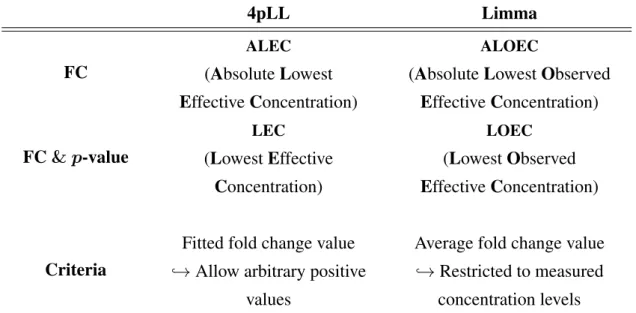
To this date, differential expression analysis was only performed using the classical naïve approach, where for each measured concentration separately it is tested if the critical effect level is exceeded (Limma t-test). This procedure has the disadvantage that only measured concentrations can be considered as potential candidates for alert concentrations . But in practice, it is highly unlikely that such a deregulation is first triggered at exactly one of the measured concentrations. To this end, a model-based method is introduced which allows arbitrary positive values as alert levels.
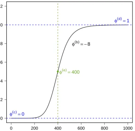
Dose-response models are used in various application fields, such as pharmacology, pharma-cokinetics, toxicology and clinical research. Typically, dose-response data exhibit a monotonic relationship between dose and response which can be modeled by a parametric regression model. Often, a sigmoidal dose-response trend is observed in the data which is characterized byS-shaped curves. Besides, there are other curves which can describe the response dependency of a dose, e.g.J-shaped or invertedU-shaped curves. These kind of curves are used for describing dose-response dependencies with a so-calledhormesis effectwhich is, in toxicology, associated with low dosis effects and high dosis inhibitions. In the context of gene expression data, such curve progressions might be a hint for the use of cytotoxic concentrations which trigger cell death as response to compound exposure. However, this work addresses only the modeling of log-logistic functions which are by far the most commonly used models for describing dose-response rela-tionships of toxicological background. Besides the log-logistic model, which exists in different parameterizations, there are other models, based for example on the log-normal- or Weibull distribution, that can be equally used to describe sigmoidal dose-response dependencies (Ritz, 2010).
All methods introduced in this section are based on an application of the four-parameter log-logistic model (4pLL). The 4pLL model is fitted to the data in order to estimate the Absolute Lowest Effective Concentration (ALEC) for a fixed and pre-specified effect level which is the concentration at which a pre-specified expression change is observed. The ALEC is derived from the fitted average trend (Jiang, 2013). Due to the fact that the critical concentration (ALEC) results from a simple point estimator, the uncertainty of the effect level is entirely neglected. But as it is vital to provide confidence intervals, the method introduced by Jiang (2013) is