Simultaneous Analysis in S-PLUS: The SimultAn Package

(1)

April 2011, Volume 40, Issue 11. http://www.jstatsoft.org/

Simultaneous Analysis in

S-PLUS

: The

SimultAn

Package

Amaya Z´arraga

Universidad del Pa´ıs Vasco/ Euskal Herriko Unibertsitatea

Beatriz Goitisolo

Universidad del Pa´ıs Vasco/ Euskal Herriko Unibertsitatea

Abstract

In this paper we describe the SimultAn package dedicated to simultaneous analysis.

Simultaneous analysis is a new factorial methodology developed for the joint treatment of a set of several data tables. Since the first stage of simultaneous analysis requires a correspondence analysis of each table the package comprises two parts, one for correspon-dence analysis and one for simultaneous analysis. The package can be used to perform classical correspondence analysis of frequency/contingency tables as well as to perform simultaneous analysis of a set of frequency/contingency tables. In this package, functions for computation, summaries and graphical visualization in two dimensions are provided, including options to display partial rows and supplementary points.

Keywords: correspondence analysis, simultaneous analysis, contingency tables, singular value

decomposition.

1. Introduction

In this paper we present theSimultAnpackage, a package for simultaneous analysis (SA) with

S-PLUS (Insightful Corp. 2003). The main reason for developing this package is to provide users with a tool for applying this new methodology which is not available elsewhere.

SA is a factorial method developed for the joint treatment of a set of several data tables, especially frequency tables whose row margins are different, for example when the tables are from different samples or different time points, without modifying the internal structure of each table. In the data tables rows must refer to the same entities, but columns may be different.

SA combines the basic idea of intra-analysis (Escofier and Drouet 1983) to maintain the internal structures of each contingency table in overall analysis and certain characteristics of

(2)

multiple factor analysis (MFA) (Escofier and Pag`es 1984, 1998) to balance the influence of the tables in the overall analysis and provides a joint description of the different structures contained within each table as well as a comparison of them.

More details about this method and its several applications can be found inGoitisolo (2002) and inZ´arraga and Goitisolo(2002,2003,2006,2008)

TheSimultAn package contains the following functions: CorrAn and SimAn, which allow the

user to perform correspondence analysis (CA) and SA, respectively. Despite there being seve-ralS-PLUSfunctions to perform data analysis (Everitt 2005), (Heiberger and Holland 2004), (Crawley 2002) as well as to perform CA (Beh 2003), (Venables and Ripley 1999), (Everitt

1994) theCorrAnfunction is implemented in the package because the first stage of SA entails

a CA of each frequency or contingency table. Nevertheless, users can perform the CA of any table or even of the concatenation of the tables. If the user wants to perform a direct SA of all the tables, there is no need first to perform the CA of each table since CorrAn is also implemented inSimAn. Thesummary.CorrAnandplot.CorrAnandsummary.SimAnand

plot.SimAnfunctions give summaries and graphical representations of CA and SA,

respec-tively.

This paper consists of three further sections. Section2briefly describes simultaneous analysis. Section3 demonstrates the application of the parameters of CorrAn and SimAn, what values they can take and what the parameters do. Section4 provides some concluding remarks. The package has been written usingS-PLUSversion 6.2 (Insightful Corp. 2003) for Windows (Professional Edition). The basics of S-PLUScan be found inKrause and Olson (2002).

2. Simultaneous analysis

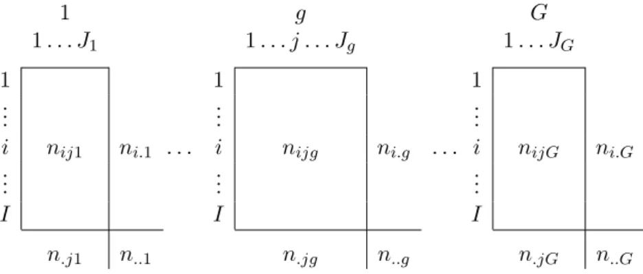
LetG={1, . . . , g, . . . , G}be the set of contingency tables to be analyzed (Figure 1).

Each of them classifies the answers ofn..g individuals with respect to two categorical variables.

All the tables have one of the variables in common, in this case the row variable with categories

I={1, . . . , i, . . . , I}. The other variable of each contingency table can be different or the same variable observed at different time points or in different subsamples. On concatenating all these contingency tables, a joint set of columnsJ={1, . . . , j, . . . , J}is obtained. The element nijg corresponds to the total number of individuals who simultaneously choose the categories

i ∈ I of the first variable and j ∈ Jg of the second variable, for table g ∈ G. Sums are

1 g G

1. . . J1 1. . . j . . . Jg 1. . . JG

1 1 1

..

. ... ...

i nij1 ni.1 . . . i nijg ni.g . . . i nijG ni.G

..

. ... ...

I I I

n.j1 n..1 n.jg n..g n.jG n..G

(3)

denoted in the usual way, for example,ni.g=Pj∈Jgnijg, andndenotes the grand total of all Gtables.

In order to maintain the internal structure of each tableG, SA begins by obtaining the relative frequencies of each table as usually done in CA:

f_ijg = nijg n..g , (1) so thatP i∈I P j∈Jgf g

ij = 1 for each tableg.

SA is carried out in two stages.

2.1. Stage one: CA of each contingency table

Because in SA it is important for each table to maintain its own structure, the first stage carries out a classical CA of each of theG contingency tables. The separate analyses of the Gtables also allow us to check for the existence of structures common to the different tables. From these analyses it is possible to obtain the weighting used in the next stage.

CA is a well-known exploratory multivariate technique for the graphical and numerical anal-ysis of contingency tables. The bibliography of publications on CA is so wide that we will not focus on its methodology. We direct interested readers to various texts where CA is described, notably Benz´ecri (1973, 1992), Greenacre (1984, 1993), Lebart, Morineau, and

Warwick (1984) andLebart, Morineau, and Piron (2006).

CA on thegth contingency table can be carried out by calculating the singular value decom-position (SVD) of the matrix Xg, whose general term is:

q f_i.g f g ij−f g i. f g .j f_i.g f_.jg ! q f_.jg. (2)

LetDg_r andDg_c be the diagonal matrices whose diagonal entries are respectively the marginal row frequenciesf_i.g and column frequenciesf_.jg. From the SVD of each tableXg we retain the first squared singular value (or eigenvalue, or principal inertia), denoted byλg₁.

2.2. Stage two: Joint analysis of the tables

In the second stage, in order to balance the influence of each table in the joint analysis, as measured by the inertia, and to prevent the joint analysis from being dominated by a particular table, SA includes a weighting on each table,αg. The choice of the weightingαg depends on

the aims of the analysis and on the initial structure of the information, and different values may be used (Z´arraga and Goitisolo 2006). The most frequently used isαg = 1/λg1, whereλ

g

1

denotes the first eigenvalue (square of first singular value) of tableg.

As a result, SA proceeds by performing a principal component analysis (PCA) of the matrix: X =h√α1X1 . . . √ αgXg . . . √ αGXG i . (3)

(4)

The PCA results are also obtained using the SVD of (3), giving singular values√λson thesth

dimension and corresponding left and right singular vectorsus andvs.The squared singular

values or eigenvalues are called principal inertias in the context of CA and their sum P sλs

is equal to the total inertia or total variance in the data table.

The projections on thesth axis of the columns are calculated as principal coordinates:

Gs = p

λsD−c1/2 vs, (4)

where Dc (J ×J), is a diagonal matrix of all the column masses, that is all theDgc.

One of the aims of the joint analysis of several data tables is to compare them through the points corresponding to the same row in the different tables. These points are referred to here

aspartial rowsand denoted byig_.

The projection on the sth axis of each partial row is denoted by Fs(ig) and the vector of

projections of all the partial rows for table gis denoted by F(sg):

F(_sg) = (Dg_r)−1/2

0 . . . √αgXg . . .0 vs. (5)

Comparison of partial rows is complicated, especially when the number of tables is large. Therefore each partial row is compared with the (overall) row, projected as:

Fs = (Dw)−1 h√ α1X1 . . . √ αgXg . . . √ αGXG i vs = (Dw)−1 X vs, (6)

where Dw is the diagonal matrix whose general term is Pg∈G

q

f_i.g. The choice of this matrixDw allows us to expand the projections of the (overall) rows to keep them inside the

corresponding set of projections of partial rows, and is appropriate when the partial rows have different weights in the tables. With this weighting, the projections of the overall and partial rows are related as follows:

Fs(i) = X g∈G q f_i.g X g∈G q f_i.g Fs(ig). (7)

Thus, the projection of a row is a weighted average of the projections of partial rows. It is closer to those partial rows that are more similar to the overall row in terms of the relation expressed by the axis and have a greater weight than the rest of the partial rows. The dispersal of the projections of the partial rows with regard to the projection of their (overall) row indicates discrepancies between the same row in the different tables.

Notice that if f_i.g is equal in all the tables, thenFs=Pg∈GG1F

(g)

s , that is, the overall row is

projected as the average of the projections of the partial rows.

The projection of a partial row on axis sis, except for the factorqαg/λs, the centroid of the

projections of the columns of table g: Fs(ig) = √ αg √ λs X j∈Jg f_ijg f_i.g Gs(j). (8)

(5)

The projection of an overall row on axissis, except for the coefficientsqαg/λs, the weighted

average of the centroids of the projections of the columns for each table:

Fs(i) = X g∈G r_α g λs q f_i.g X g∈G q f_i.g   X j∈Jg f_ijg f_i.g Gs(j)  . (9)

To compare the different tables, SA provides measurements of the relation between the factors of the different analyses. For seeking the relation between factors of the individual CA of the tables, the correlation coefficient can be used to measure the degree of similarity between the factors of the separate CA of different tables. This is possible when the marginals f_i.g are equal.

The relation between the factorssands0of the tablesgandg0respectively would be calculated with the correlation coefficient:

rFg_s,Fg_s00 = X i∈I F_sg(i) √ λgs f_i.g F g0 s0(i) q λg_s00 , (10)

where F_sg(i) and F_sg00(i) are the projections on the axes s and s0 of the separate CA of the

tablesgand g0 respectively and whereλg_s and λg_s00 are the inertias associated with these axes.

When f_i.g are not equal, the generalized correlation (Z´arraga and Goitisolo 2003) is used to calculate the relation between the factors sand s0 of the tables gand g0 respectively:

rFg_s,Fg_s00 = X i∈I F_sg(i) √ λgs q f_i.g q f_i.g0 F g0 s0(i) q λg_s00 . (11)

This measurement allows us to verify whether the factors of the separate analyses are similar and check the possible rotations that occur.

Likewise, it is possible to calculate for each factor s of the SA the relation with each of the factors s0 of the CA separate analyses of the different tables:

r Fg_s0,Fs = X i∈I F_sg0(i) q λg_s0 q f_i.g   X g∈G q f_i.g   F_√s(i) λs . (12)

If all the analyzed frequency tables have the same row weights this measurement is reduced to: r Fg_s0,Fs = X i∈I f_i.g F_sg0(i) Fs(i) s X i∈I f_i.g F_sg0(i) 2 s X i∈I f_i.g (Fs(i))2 , (13)

that is the classical correlation coefficient between the factors of the separate CA and the factors of SA.

(6)

The relation between the overall rows and the partial rows can be calculated in order to verify whether a table is well represented in each of the factors of the simultaneous analysis. The generalized correlation between the projections of the partial rows,F(sg), and the projections

of the overall rows,Fs, is calculated as:

rF(_sg),Fs = X i∈I q f_i.g Fs(ig) s X i∈I f_i.g(Fs(ig))2   X g∈G q f_i.g   Fs(i) p λs . (14)

By considering the tables as groups of columns, in the sense of MFA (Escofier and Pag`es 1998), it may be also interesting to project the tables on the axes of SA. The projection of table g onto thesth axis,Hs(g), is obtained as:

Hs(g) = X j∈Jg

f_.jg G2_s(j) = Inertias(g), (15)

where Inertias(g) represents the sum of the projected inertias of columns of tableg on axiss.

Because of the weighting αg = 1/λg1, the projections Hs(g) take values between 0 and 1

and the contributions of each table to the formation of the axiss, Hs(g)/λs, show that the

influence of the tables in the joint analysis is balanced.

A value ofHs(g) close to 1 would indicate that the axis of the joint analysis is a direction of

major inertia for tableg, whereas a weak value would indicate that the axis is a direction of very weak inertia for tableg.

Consequently, adding the projections of all the tables gives the projected inertia on the axis:

X g∈G Hs(g) = X g∈G Inercias(g) =λs. (16)

As the projection of each group on the first axis is less than or equal to one, the projected inertia onto it is between zero andG, the number of tables.

3. Application

To illustrate the outputs and graphs of SimultAn we show two examples – one for CA and one for SA – using the traffic.dat dataset, which is available in the package. The dataset contains the number of drivers involved in road accidents with fatalities in 2005, classified according to the age and sex of the drivers and the vehicles involved. This information is taken from the Spanish Traffic Authority: http://www.dgt.es/portal/es/seguridad_ vial/estadistica/accidentes_30dias/datos_desagregados.do (Grupo 4 – 2005, on Sheet 4.2.C).

The categories of vehicles driven are the following: Bicycles, mopeds, motorcycles, public service cars up to 9 seats, private cars, vans, trucks weighing less than 3500 kg, agricultural tractors, trucks and articulated vehicles weighing more than 3500 kg, buses and other un-specified vehicles. The age categories envisaged in the study are the following: 18 to 20, 21 to 24, 25 to 34, 35 to 44, 45 to 54, 55 to 64, 65 to 74, over 74 years and unknown age (UA).

(7)

The labels of the age categories are preceded byMandFto distinguish which table they belong to (i.e.,M18to20for males andF18to20 for females).

In order to study the interaction between the kind of vehicle driven and the driver’s age group for each gender we consider the analysis of two tables, one for each gender, where the 11 rows correspond to the kinds of vehicle driven and the 9 columns to the drivers’ age groups.We therefore have one table for the 57420 male drivers and another for the 12573 female drivers involved in road accidents (Z´arraga and Goitisolo 2009).

The SimultAn package comprises two parts. The first is for the classical CA of each of

the two tables or the classical CA of the concatenation of the tables including (or not) the supplementary elements. TheCorrAn function computes the CA. The second part allows the simultaneous analysis of the two tables to be performed using theSimAnfunction.

3.1. Correspondence analysis

The first step in the analysis is to read the dataset and select the rows and columns to be used as active or supplementary elements in the analysis.

The instruction for reading the data is:

S> data <- read.table(file = "traffic.dat")

The instruction for selecting rows and columns from the dataset depends on the aim of the user. Let us assume that the user is interested in analysing the table corresponding to male drivers as active, i.e., all 11 rows corresponding to vehicles and the first 9 columns corresponding to the ages of male drivers.

The selection of the data would be:

S> dataCA <- data[1:11, 1:9]

TheCorrAn function computes the CA of the selected data. The instruction to perform the

CA is:

S> CorrAn.out <- CorrAn(data = dataCA)

The following output of CA is given by

S> summary(CorrAn.out)

$"Total inertia": Total inertia

0.09032129

$"Eigenvalues and percentages of inertia": values percentage cumulated

s=1 0.0559327 61.9264161 61.92642

s=2 0.0154225 17.0751337 79.00155

s=3 0.0086134 9.5363933 88.53794

(8)

s=5 0.0019874 2.2003224 99.71335

s=6 0.0001531 0.1694929 99.88284

s=7 0.0000886 0.0980538 99.98090

s=8 0.0000173 0.0191048 100.00000

s=9 0.0000000 0.0000000 100.00000

corresponding to the total inertia, as a measure of the total variance of the data table, to the eigenvalues or principal inertias as well as to the percentages of explained inertia and cumulated percentages of explained inertia for all possible dimensions.

The output also contains, for rows and columns, the masses in %(100fi, 100fj), the chi-squared distances of points to their average (d2) and, by default restricted to the first two dimensions s = 1, 2, the projections of points on each dimension or principal coordinates (Fs, for rows, Gs for columns), contributions of the points to the dimensions and squared correlations (ctrsand cors, respectively).

$"Output for rows":

100fi d2 F1 F2 ctr1 ctr2 cor1 cor2

Bicycle 1.14 0.25 0.04 0.40 0.03 11.58 0.01 0.63 Moped 3.64 0.80 0.83 -0.09 44.85 1.98 0.86 0.01 Motorcycle 6.56 0.23 -0.31 -0.34 11.10 48.89 0.42 0.50 Car,PS 0.65 0.08 -0.13 0.23 0.20 2.32 0.21 0.68 Private car 65.39 0.01 0.08 -0.01 6.74 0.12 0.69 0.00 Van 8.28 0.03 -0.14 0.07 3.11 2.28 0.66 0.13 Truck-3500 3.24 0.11 -0.31 0.03 5.63 0.20 0.86 0.01 Tractor 0.58 0.56 0.11 0.61 0.12 13.78 0.02 0.66 Truck+3500 8.13 0.21 -0.42 0.07 25.86 2.61 0.85 0.02 Bus 0.72 0.25 -0.43 0.16 2.34 1.26 0.73 0.11 Other 1.67 0.54 -0.03 0.37 0.02 15.00 0.00 0.26

$"Output for columns":

100fj d2 G1 G2 ctr1 ctr2 cor1 cor2 M18to20 5.65 0.59 0.72 -0.11 52.73 4.26 0.89 0.02 M21to24 10.67 0.06 0.18 -0.06 6.44 2.51 0.57 0.06 M25to34 29.68 0.03 -0.09 -0.13 4.37 34.81 0.28 0.61 M35to44 21.76 0.03 -0.17 0.01 10.83 0.08 0.85 0.00 M45to54 14.56 0.04 -0.16 0.11 6.55 10.89 0.58 0.27 M55to64 9.18 0.04 -0.01 0.19 0.01 20.45 0.00 0.79 M65to74 4.98 0.20 0.35 0.20 10.94 13.54 0.60 0.21 M75plus 1.95 0.30 0.48 0.14 8.12 2.58 0.78 0.07 MUA 1.57 0.56 -0.02 0.33 0.01 10.89 0.00 0.19

All the arguments of theCorrAn function can be consulted by the function names():

(9)

which gives the parameters:

"data" "sr" "sc" "nd" "dp"

The CorrAn function offers the inclusion of supplementary elements, the parameters sr and

scindicate the supplementary rows and supplementary columns, respectively. The parameter

ndindicates the dimensionality of the solution, which by default isnd = 2, and the parameter

dpindicates the number of decimal places for numerical results, which by default is dp = 2, except for eigenvalues and percentages of inertia.

Assume that the CA is performed on the traffic data where the category of vehicle Other

(i.e., the eleventh row) and the category of unknown age for males driversMUA(i.e., the ninth column) are treated as supplementary points. The instruction to perform this CA is:

S> CorrAn.out <- CorrAn(data = dataCA, sr = 11, sc = 9)

In the corresponding section of the output of

S> summary(CorrAn.out)

the following results for the supplementary elements are given:

$"Output for supplementary rows":

100fi d2 F1 F2 cor1 cor2

Other 1.55 0.04 0.02 0.16 0.01 0.65

$"Output for supplementary columns":

100fj d2 G1 G2 cor1 cor2

MUA 1.44 0.03 0.01 0.04 0 0.06

Supplementary points have no influence in the calculation of the axes. They are projected onto the axes afterwards. Thus, contributions are not applicable for these points but squared correlations are meaningful measures of how well supplementary elements are represented by the axes.

The graphical representation of the results of CA is created with the following instruction:

S> plot(CorrAn.out, s1 = 1, s2 = 2)

where the parameters s1 = 1 and s2 = 2 indicate that the graph is given for the first two dimensions. A plot of e.g., the second and the third dimensions is obtained by setting s1

= 2 and s2 = 3. Notice that in this case the argument nd of the CorrAn function must

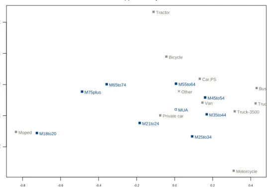
be at least 3. If there are supplementary elements in the analysis, theplot.CorrAnfunction provides two graphical outputs, one for the active elements and the second one for both active and supplementary elements. Figure2shows the display of active and supplementary points in the first two dimensions.

A list of all available results given byCorrAn()can be obtained with the instruction:

(10)

-0.8 -0.6 -0.4 -0.2 0.0 0.2 0.4 -0.2 0.0 0 .2 0.4 0 .6

CA

Axis 1 ( 69.14 %) Axis 2 ( 17.69 %)

Active and supplementary elements

Bicycle Moped Motorcycle Car,PS Private car Van Truck-3500 Tractor Truck+3500 Bus M18to20 M21to24 M25to34 M35to44 M45to54 M55to64 M65to74 M75plus Other MUA

Figure 2: Correspondence analysis: Active and supplementary elements.

The output is structured as a list object:

totalin Total inertia.

eig Eigenvalues.

resin Results of inertia.

resi Results of active rows.

resj Results of active columns.

resisr Results of supplementary rows.

resjsc Results of supplementary columns.

X Matrix X to be diagonalized.

totalk Total of data table.

I Number of active rows.

(11)

fi Marginal of active rows.

Fs Projections of active rows.

d2i Chi-square distance of active rows to their average.

J Number of active columns.

namej Names of active columns.

fj Marginal of active columns.

Gs Projections of active columns.

d2j Chi-square distance of active columns to their average.

Isr Number of supplementary rows.

nameisr Names of supplementary rows.

fisr Marginal of supplementary rows.

Fssr Projections of supplementary rows.

d2isr Chi-square distance of supplementary rows to the average.

Xsr Matrix X for supplementary rows.

Jsc Number of supplementary columns.

namejsc Names of supplementary columns.

fjsc Marginal of supplementary columns.

Gssc Projections of supplementary columns.

d2jsc Chi-square distance of supplementary columns to the average.

and the values of all the objects are obtained with:

S> CorrAn.out

The value of each object, for example the total inertia of the table, is obtained with:

S> CorrAn.out$totalin

3.2. Simultaneous analysis

In order to perform the SA of a set of tables, after reading the data with the instruction:

(12)

it is necessary to select which tables are to be jointly analyzed and which are the active and supplementary elements (if any).

Remember that the traffic.dat dataset contains two tables, one for each gender, where the 11 rows correspond to the kinds of vehicle driven and the 18 columns to the drivers’ age groups. Columns 1 to 9 correspond to male drivers’ age groups and columns 10 to 18 to female drivers’ age groups.

The SimAnfunction computes the SA of the tables:

S> SimAn.out <- SimAn(data = dataSA, G = 2, acg = list(1:9, 10:18), + weight = 2, nameg = c("M", "F"))

where data = dataSA indicates which data set is to be analyzed, the parameter Gindicates the number of tables to be jointly analyzed, G = 2 in this example, and acg indicates the active columns of each table. The parameterweight refers to the weightingαg (Section2.2).

Three values are possible, weight = 1means αg = 1,weight = 2 means αg = 1/λg1, where

λg₁denotes the first eigenvalue (square of first singular value) of tablegand is given by default,

and weight = 3 meansαg = 1/Total Inertia (g). Since in SA the rows are the same for all

the tables, the parameter nameg allows the user to distinguish in the interpretation of the results as well as in the graphical representations which partial rows belong to each table. In this example we have chosenMfor the first table, the table of male drivers, and Ffor the second one, the table of female drivers. By default, if this parameter is not indicated, partial rows of the first table will be identified asG1 followed by the name of the row, partial rows of the second table as G2 followed by the name of the row and so on. The nameg argument also allows the different tables in the analysis to be identified.

More optional arguments for theSimAn() function include an option for setting the dimen-sionality of the solution (nd), an option for setting the number of decimal places for numerical results (dp) and options for selecting rows and /or columns as supplementary elements (sr

andsc, respectively). By default, the parameters nd and dptake the value 2. All the above parameters are given by:

S> names(SimAn)

The following instruction gives the summary output ofSimAn:

S> summary(SimAn.out)

In its first stage SA performs a CA of each table (Section 2.1), so the output contains the separate CA of each table, as provided by the CorrAn function in Section 3.1, i.e., total inertia, explained inertias by the dimensions and, for rows and columns, the masses, distances, principal coordinates, contributions of the points to the dimensions and squared correlations. The following output is given for the table of male drivers (table M) and for the table of female drivers (table F):

[1]"CA table M" $"Total inertia":

Total inertia 0.09032129

(13)

s=1 0.0559327 61.9264161 61.92642

s=2 0.0154225 17.0751337 79.00155

s=3 0.0086134 9.5363933 88.53794

...

s=9 0.0000000 0.0000000 100.00000

$"Output for rows":

MBicycle 1.14 0.25 0.04 0.40 0.03 11.58 0.01 0.63

MMoped 3.64 0.80 0.83 -0.09 44.85 1.98 0.86 0.01

MMotorcycle 6.56 0.23 -0.31 -0.34 11.10 48.89 0.42 0.50

...

MOther 1.67 0.54 -0.03 0.37 0.02 15.00 0.00 0.26

100fj d2 G 1 G 2 ctr1 ctr2 cor1 cor2 M18to20 5.65 0.59 0.72 -0.11 52.73 4.26 0.89 0.02 M21to24 10.67 0.06 0.18 -0.06 6.44 2.51 0.57 0.06 M25to34 29.68 0.03 -0.09 -0.13 4.37 34.81 0.28 0.61 ... MUA 1.57 0.56 -0.02 0.33 0.01 10.89 0.00 0.19 "CA table F" $"Total inertia": Total inertia 0.03389271

s=1 0.0219155 64.6612977 64.66130

s=2 0.0057888 17.0797638 81.74106

...

s=9 0.0000000 0.0000000 100.00000

$"Output for rows":

FBicycle 0.45 0.75 -0.04 -0.82 0.03 51.56 0.00 0.89

FMoped 2.42 0.83 0.91 -0.02 91.29 0.13 1.00 0.00

FMotorcycle 0.88 0.20 -0.17 0.12 1.22 2.14 0.15 0.07

...

FOther 0.93 0.23 0.00 -0.36 0.00 21.10 0.00 0.57

(14)

F18to20 5.33 0.33 0.57 -0.02 79.67 0.55 1.00 0.00

F21to24 13.23 0.02 0.10 0.06 5.95 8.47 0.57 0.21

F25to34 36.86 0.00 -0.04 0.04 2.78 10.41 0.36 0.35

...

FUA 1.39 0.15 -0.02 -0.24 0.03 13.53 0.00 0.38

The joint analysis of all the tables is performed in the second stage of the SA (Section 2.2). The output of SimAn contains the total inertia, the eigenvalues, percentages of explained inertia and cumulated percentages of explained inertia for all dimensions.

$"Total inertia": [1] 3.16134

s=1 1.7681305 55.9297826 55.92978 s=2 0.4723711 14.9421178 70.87190 s=3 0.4360638 13.7936387 84.66554 s=4 0.2372980 7.5062463 92.17179 s=5 0.1105581 3.4971907 95.66898 s=6 0.0596409 1.8865696 97.55555 s=7 0.0394521 1.2479561 98.80350 s=8 0.0198511 0.6279337 99.43144 s=9 0.0101133 0.3199042 99.75134 s=10 0.0071411 0.2258888 99.97723 s=11 0.0007199 0.0227715 100.00000

In SA, with the weight used by default αg = 1/λg1, the total inertia is a weighted average of

the inertias of the tables and the first eigenvalue takes values between 1 and the number of tables, in this case 2. The first eigenvalue is 1.77, close to its maximum value of 2. This value indicates that the first axis of the SA is an axis of major inertia in the two data tables. As with simple CA (Section 3.1), the output also contains, for the overall rows and for the columns of the two tables, the masses (pi, 100fjg), chi-squared distances (d2) and, by default restricted to the first two dimensions s = 1, 2, projections of points on each dimension or principal coordinates (Fs, for rows,Gs, for columns), contributions of the points to the dimensions and squared correlations (ctrsand cors, respectively).

$"Output for rows":

pi d2 F1 F2 ctr1 ctr2 cor1 cor2 Bicycle 0.03 6.74 0.11 2.18 0.02 30.34 0.00 0.71 Moped 0.12 12.01 -3.38 0.02 77.30 0.01 0.95 0.00 Motorcycle 0.12 2.85 0.87 -0.97 5.21 24.62 0.26 0.33 Car,PS 0.02 1.70 0.06 0.87 0.01 4.00 0.00 0.45 Private car 3.10 0.04 -0.06 -0.04 0.58 1.31 0.09 0.05 Van 0.22 0.71 0.56 0.30 3.90 4.09 0.44 0.12 Truck-3500 0.06 1.69 0.98 -0.02 3.05 0.01 0.57 0.00 Tractor 0.01 8.47 0.43 1.77 0.11 6.82 0.02 0.37

(15)

Truck+3500 0.12 2.86 1.08 0.32 7.98 2.61 0.41 0.04

Bus 0.02 4.36 1.43 0.17 1.84 0.10 0.47 0.01

Other 0.05 5.05 0.06 1.55 0.01 26.09 0.00 0.48

100fjg d2 G1 G2 ctr1 ctr2 cor1 cor2 M18to20 5.65 10.47 -3.21 -0.24 32.83 0.66 0.98 0.01 M21to24 10.67 1.06 -0.55 -0.37 1.81 3.12 0.28 0.13 M25to34 29.68 0.53 0.36 -0.51 2.18 16.58 0.25 0.50 M35to44 21.76 0.59 0.55 0.06 3.74 0.15 0.52 0.01 M45to54 14.56 0.77 0.58 0.39 2.77 4.65 0.44 0.20 M55to64 9.18 0.78 0.14 0.59 0.10 6.79 0.02 0.45 M65to74 4.98 3.64 -1.03 0.81 3.00 6.96 0.29 0.18 M75plus 1.95 5.32 -1.68 0.66 3.11 1.80 0.53 0.08 MUA 1.57 10.06 -0.01 1.84 0.00 11.28 0.00 0.34 F18to20 5.33 15.02 -3.60 0.18 39.16 0.35 0.86 0.00 F21to24 13.23 0.79 -0.75 -0.27 4.21 2.02 0.71 0.09 F25to34 36.86 0.21 0.25 -0.30 1.34 7.03 0.31 0.43 F35to44 22.78 0.37 0.42 -0.04 2.30 0.09 0.48 0.00 F45to54 13.10 0.72 0.56 0.24 2.36 1.56 0.44 0.08 F55to64 5.11 2.07 0.59 1.18 1.02 14.98 0.17 0.67 F65to74 1.68 3.55 -0.15 1.08 0.02 4.16 0.01 0.33 F75plus 0.52 24.30 -0.36 3.25 0.04 11.56 0.01 0.43 FUA 1.39 6.71 0.10 1.46 0.01 6.25 0.00 0.32

Partial rows only play a role in the analysis in building the overall rows and are projected (Fs) as supplementary elements. Therefore they do not contribute, on their own, to the axes but squared correlations (cors) are still meaningful measures of how well they are represented by the axes and are included in the output. Notice how the parameter nameg = c("M", "F")

allows the partial rows of each table to be identified by putting anMand anFbefore the name of the rows.

$"Output for partial rows":

100fig d2 F1 F2 cor1 cor2

MBicycle 1.14 4.43 -0.04 1.26 0.00 0.36 MMoped 3.64 14.39 -2.60 -0.04 0.47 0.00 MMotorcycle 6.56 4.08 0.85 -0.98 0.18 0.24 MCar,PS 0.65 1.45 0.39 0.69 0.11 0.33 MPrivate car 65.39 0.15 -0.20 -0.03 0.28 0.01 MVan 8.28 0.57 0.42 0.15 0.32 0.04 MTruck-3500 3.24 2.03 0.87 0.07 0.37 0.00 MTractor 0.58 10.00 -0.14 1.71 0.00 0.29 MTruck+3500 8.13 3.74 1.18 0.17 0.38 0.01 MBus 0.72 4.47 1.21 0.43 0.33 0.04 MOther 1.67 9.57 0.09 1.42 0.00 0.21 FBicycle 0.45 34.20 0.35 3.66 0.00 0.39 FMoped 2.42 37.91 -4.33 0.09 0.49 0.00

(16)

FMotorcycle 0.88 9.32 0.91 -0.95 0.09 0.10 FCar,PS 0.60 5.53 -0.28 1.06 0.01 0.20 FPrivate car 90.45 0.02 0.07 -0.06 0.19 0.16 FVan 3.35 3.30 0.77 0.52 0.18 0.08 FTruck-3500 0.31 9.05 1.36 -0.33 0.20 0.01 FTractor 0.06 45.51 2.13 1.97 0.10 0.09 FTruck+3500 0.38 10.34 0.61 1.02 0.04 0.10 FBus 0.17 21.57 1.87 -0.36 0.16 0.01 FOther 0.93 10.45 0.03 1.74 0.00 0.29

The output of summary.SimAn also contains the relations between overall rows and partial rows, the relations between the factors of the CA of the different tables, the relations between the factors of the SA and the factors of the separate CA of the different tables, the projections of the tables and the contributions of each table to the principal axes (Section2.2).

TheSimAnfunction also allows supplementary elements (rows and/or columns) to be included

in the analysis. Assume that row 11 (category of vehicleOther) takes part in the analysis as a supplementary row.

The instruction to perform this SA is:

S> SimAn.out <- SimAn(data = dataSA, G = 2, acg = list(1:9, 10:18), + weight = 2, nameg = c("M", "F"), sr = 11)

In the corresponding section of the output of

S> summary(SimAn.out)

the following results for the overall supplementary row and for supplementary partial rows are given:

$"Output for supplementary rows":

pi d2 F1 F2 cor1 cor2

Other 0.05 5.49 -0.05 0.08 0 0

$"Output for supplementary partial rows":

100fig d2 F1 F2 cor1 cor2

MOther 1.70 10.72 -0.08 0.04 0 0

FOther 0.94 10.79 -0.01 0.14 0 0

The graphical representation of the results from SA is created with the following instruction:

S> plot(SimAn.out, s1 = 1, s2 = 2)

where the parameters s1 = 1 and s2 = 2 (by default) indicate that the graph is given for the first two dimensions. A plot of e.g., the second and the third dimensions is obtained by setting s1 = 2 and s2 = 3. Notice that in the latter case nd, the dimensionality of the solution, must be at least 3. A large number of elements can take part in the SA of a set of tables depending on the number of tables and on the dimensions of the tables. In order to facilitate interpretation, the plot.SimAn function gives several graphical outputs for active

(17)

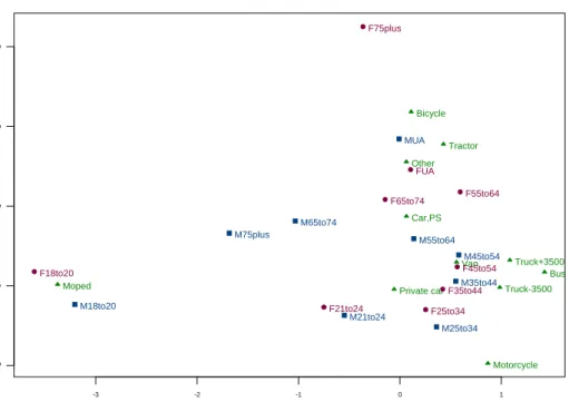
-3 -2 -1 0 1 -1 0 1 2 3

SA: Overall rows and columns

Axis 1 ( 55.93 %) A x is 2 ( 1 4 .9 4 % ) Active elements Bicycle Moped Motorcycle Car,PS Private car Van Truck-3500 Tractor Truck+3500 Bus Other M18to20 M21to24 M25to34 M35to44 M45to54 M55to64 M65to74 M75plus MUA F18to20 F21to24 F25to34 F35to44 F45to54 F55to64 F65to74 F75plus FUA

Figure 3: Simultaneous analysis: Active rows and columns.

-4 -3 -2 -1 0 1 2 -1 0 1 2 3

SA: Overall and partial rows

Axis 1 ( 55.93 %) A x is 2 ( 1 4 .9 4 % ) Active elements Bicycle Moped Motorcycle Car,PS Private car Van Truck-3500 Tractor Truck+3500 Bus Other MBicycle MMoped MMotorcycle MCar,PS

MPrivate car MVan MTruck-3500 MTractor MTruck+3500 MBus MOther FBicycle FMoped FMotorcycle FCar,PS FPrivate car FVan FTruck-3500 FTractor FTruck+3500 FBus FOther

(18)

0.0 0.2 0.4 0.6 0.8 1.0 0.0 0.2 0.4 0.6 0.8 1.0

SA: Tables

Axis 1 ( 55.93 %) A x is 2 ( 1 4 .9 4 % ) M F

Figure 5: Simultaneous analysis: Projections of the tables.

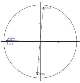
Relation between factors of CA and SA

Axis 1 ( 55.93 %) A x is 2 ( 1 4 .9 4 % ) F1(M) F1(F) F2(M) F2(F)

(19)

and supplementary points (if any) including the ones corresponding to the separate CA of each table. Figures3and4 show, for the analysis in which all the points are active elements, the displays of overall rows and columns and overall rows and partial rows, respectively. Each table is identified with a different color and the columns and partial rows of each table are in the same color and have the same symbol.

Two additional graphs, one for the projections of the tables (Figure5) and one for the relations between factors of CA and SA (Figure6) are also provided by plot.SimAn.

A list of all available results given bySimAn() can be obtained with the instruction:

S> names(SimAn.out)

The output is structured as a list object:

totalin Total inertia.

resin Results of inertia.

resi Results of active rows.

resig Results of partial rows.

resj Results of active columns.

Fsg Projections of each table.

ctrg Contribution of each table to the axes.

riig Relation between the overall rows and the partial rows.

rCACA Relation between separate CA axes.

rCASA Relation between CA axes and SA axes.

Fsi Projections of active rows.

Fsig Projections of partial rows.

Gs Projections of active columns.

allFs Projections of rows and partial rows in an array format.

allGs Projections of columns in an array format.

I Number of active rows.

maxJg Maximum number of columns for a table.

G Number of tables.

namei Names of active rows.

nameg Prefix for identifying partial rows, tables, etc.

(20)

resigsr Results of partial supplementary rows.

Fsisr Projections of supplementary rows.

Fsigsr Projections of partial supplementary rows.

allFssr Projections of rows and partial supplementary rows in an array format.

Isr Number of supplementary rows.

nameisr Names of supplementary rows.

resjsc Results of supplementary columns.

Gssc Projections of supplementary columns.

allGssc Projections of supplementary columns in an array format.

Jsc Number of supplementary columns.

namejsc Names of supplementary columns.

CAret Results of CA of each table to be used in summary and plot functions.

4. Conclusion

We have presented the SimultAn package for simultaneous analysis of a set of contingency tables not available elsewhere. This package also allows the user to perform correspondence analysis of any table, of any combination of tables and even of the concatenation of all tables. All the features of the package are explained and illustrated in this paper using the dataset

traffic.dat, which is available in the package.

Acknowledgments

This work has been supported by the Basque Government under UPV/EHU research grant IT-347-10.

References

Beh EJ (2003). “S-PLUSCode for Simple and Multiple Correspondence Analysis.”

Computa-tional Statistics,20, 415–438.

Benzécri JP (1973). L’ Analyse des Données: L’ Analyse des Correspondances. Dunod, Paris. Benzécri JP (1992). Correspondence Analysis Handbook. Dekker, New York.

Crawley MJ (2002). Statistical Computing. An Introduction to Data Analysis Using S-PLUS. John Wiley & Sons, Chichester.

(21)

Escofier B, Drouet D (1983). “Analyse des Diff´erences entre Plusieurs Tableaux de Fr´equence.”

Cahiers de L’ Analyse des Donn´ees,VIII(4), 491–499.

Escofier B, Pag`es J (1984). “L’ Analyse Factorielle Multiple.”Cahiers du Bureau Universitaire

de Recherche Op´erationnelle,42, 1–68.

Escofier B, Pag`es J (1998). Analyses Factorielles Simples et Multiples. Objetifs, M´ethodes et

Interpr´etation. 2nd edition. Dunod, Paris.

Everitt BS (1994). A Handbook of Statistical Analysis Using S-PLUS. Chapman and Hall, London.

Everitt BS (2005). An Rand S-PLUS Companion to Multivariate Analysis. Springer-Verlag, London.

Goitisolo B (2002). El Análisis Simultáneo. Propuesta y Aplicación de un Nuevo Método de

An´alisis Factorial de Tablas de Contingencia. Basque Country University Press, Bilbao.

Greenacre MJ (1984).Theory and Applications of Correspondence Analysis. Academic Press, London.

Greenacre MJ (1993). Correspondence Analysis in Practice. Academic Press, London. Heiberger RM, Holland B (2004). Statistical Analysis and Data Display. An Intermediate

Course with Examples in S-PLUS, R andSAS. Springer-Verlag, New York.

Insightful Corp (2003). S-PLUS Version 6.2. Seattle, WA. URL http://www.insightful. com/.

Krause A, Olson M (2002). The Basics of S-PLUS. 3rd edition. Springer-Verlag, New York. Lebart L, Morineau A, Piron M (2006). Statistique Exploratoire Multidimensionnelle. 4th

edition. Dunod, Paris.

Lebart L, Morineau A, Warwick K (1984).Multivariate Descriptive Statistical Analysis. John Wiley & Sons, New York.

Venables WN, Ripley BD (1999). Modern Applied Statistics with S-PLUS. 3rd edition. Springer-Verlag, New York.

Zárraga A, Goitisolo B (2002). “Méthode Factorielle pour l’ Analyse Simultanée de Tableaux de Contingence.”Revue de Statistique Appliquée,L(2), 47–70.

Zárraga A, Goitisolo B (2003). “ Étude de la Structure Inter-tableaux à travers l’ Analyse Simultanée.”Revue de Statistique Appliquée,LI(3), 39–60.

Z´arraga A, Goitisolo B (2006). “Simultaneous Analysis: A Joint Study of Several Contingency Tables with Different Margins.” In M Greenacre, J Blasius (eds.),Multiple Correspondence

Analysis and Related Methods, pp. 327–350. Chapman & Hall/CRC, Boca Raton.

Z´arraga A, Goitisolo B (2008). “Factorial Analysis of a Set of Contingency Tables.” In C Preisach, H Burkhardt, L Schmidt-Thieme, R Decker (eds.), Data Analysis, Machine

Learning and Applications, Studies in Classification, Data Analysis, and Knowledge

(22)

Z´arraga A, Goitisolo B (2009). “Simultaneous Analysis and Multiple Factor Analysis for Con-tingency Tables: Two Methods for the Joint Study of ConCon-tingency Tables.”Computational

Statistics and Data Analysis,53(8), 3171–3182.

Affiliation:

Beatriz Goitisolo

Departamento de Econom´ıa Aplicada III (Econometr´ıa & Estad´ıstica) Universidad del Pa´ıs Vasco/Euskal Herriko Unibertsitatea

Avda. Lehendakari Aguirre, 83 48015 Bilbao, Spain

E-mail: [email protected]

Amaya Z´arraga

Departamento de Econom´ıa Aplicada III (Econometr´ıa & Estad´ıstica) Universidad del Pa´ıs Vasco/Euskal Herriko Unibertsitatea

Avda. Lehendakari Aguirre, 83 48015 Bilbao, Spain

E-mail: [email protected]