Fatigue life assessment on composite concrete-steel bridges

(1)

Fatigue life assessment on composite

concrete-steel bridges

Author:

Gonzalo Jurado

Supervisors: Prof. Luis Borges Prof. Carlos Rebelo Prof. Helena Gervasio

University of Coimbra

University of Coimbra Date: 31-01-2017

(2)

ACKNOWLEDGEMENTS

This work has been carried out under the supervision of Prof. Luís Borges, Prof. Carlos Rebelo and Prof. Helena Gervásio and I would like to thank them for all their help and encouragement.

I would like to thank Prof. Luís Simões da Silva, director of ISISE, for his support and for granting me the opportunity to work in an outstanding research environment. To the administrative staff (Manuela, Vera and Bárbora) whose cooperation and assistance throughout the program have been greatly appreciated. My special gratitude goes to my family for their patience and constant support. They have guided, encouraged, loved and consoled me through it all. I love you more than words can express.

To my friends, those who, despite the physical distance, have always been there for me when I needed them the most. The warmth of their words in moments of despair has meant everything to me. Thank you.

My time during SUSCOS program has been memorable thanks to all my colleagues. I would like to thank all of you for the good times we spent both at the university and outside. It has been an incredible experience and I owe it to you.

Finally, to my dear friend who is watching me from heaven.

Coímbra, 31 January 2017 Gonzalo Jurado

‘Life is not waiting for the storm to pass, it’s learning how to dance in the rain’. - Vivian Greene.

(3)

ABSTRACT

Fatigue is an important consideration in the design of bridges, especially those made of steel. Cycles resulting from the passage of a truck over a bridge depend essentially on bridge type, detail location, span length and vehicles axles configuration. Moreover, as bridges form the keystone of transport networks, their safe operation with minimal maintenance closures is paramount for efficient operation. Yearly increases in the volume of heavy traffic mean a higher number of fatigue damaging load cycles, which leads to taking appropriate measures and finding sustainable solutions, with reduced environmental, economic and social impacts.

This work is focused on developing a software tool for the design and assessment of composite concrete-steel bridges under fatigue, according to Eurocodes. The type of bridge used for this project is limited to a road-girder-bridge. Design approaches include both the damage equivalent factor method and the damage accumulation method. For the latter, an algorithm was developed which simulates truck passages over a bridge model and calculates fatigue load effects using the axle positions recorded in real time. This information could serve as an identification tool for bridges where fatigue is likely to be a problem and could form part of a full bridge management framework in the future.

Furthermore, the program is applied into a real case study, in order to compare the results and evaluate its efficiency and accuracy. Finally, conclusions are drawn and future work is proposed, leaving space for improvements and new challenges.

(4)

LIST OF FIGURES

Figure 2.1: Damage equivalent factor (Hirt, 2006). ... 3

Figure 2.2: Fatigue load model 1 according to EN 1991-2 (Al-Emrani et al., 2014). ... 4

Figure 2.3: Fatigue load model 3 according to EN 1991-2 (Al-Emrani et al., 2014). ... 5

Figure 2.4: Fatigue load models for road bridges according to EN 1991-2 (Al-Emrani et al., 2014). ... 8

Figure 2.5: Overview of the application of the λ−coefficient method (Al-Emrani et al., 2014). ... 13

Figure 2.6: Location of mid-span or support section (source EN 1993-2). ... 13

Figure 2.7: The factor λ1 for road and railway bridges as a function of the critical influence line length (Nussbaumer, 2006). ... 14

Figure 2.8: Damage equivalent factor λ1 for road bridge details (Al-Emrani et al., 2014). ... 14

Figure 2.9: Example of transverse distribution of two-girder bridge cross-section in function of lateral load positions (Al-Emrani et al., 2014). ... 16

Figure 2.10: λmax factor for road bridge sections subjected to bending stresses (Al-Emrani et al., 2014). 17 Figure 2.11: An example of variable amplitude loading and stress histogram resulting from the application of cyclic counting method (Al-Emrani et al., 2014). ... 18

Figure 2.12: The application steps of cumulative damage method (Al-Emrani et al., 2014). ... 21

Figure 2.13: Set of fatigue strength (S-N) curves for normal stress ranges (Nussbaumer et al., 2011). .... 22

Figure 2.14: Set of fatigue strength curves for shear stress ranges (Nussbaumer et al., 2011). ... 23

Figure 2.15: Moving load, Moving mass and Sprung mass models, respectively (Yang et al., 2004). ... 26

Figure 3.1: Program’s flowchart. ... 28

Figure 3.2: Mean moment vs days of analysis, considering standard deviation (example). ... 38

Figure 3.3: Equivalent spans, for effective width of concrete flange (EN 1994-2). ... 43

Figure 3.4: Iterative procedure to obtain the position of the neutral axis in class 4 cross-sections (effective). ... 45

Figure 3.5: Typical detail categories (Adapt. from “Ponts Metalliques et Miixtes” – SETRA). ... 45

Figure 3.6: Schematic of fatigue reliability assuming damage tolerant and safe life methods and a failure with high consequence (Nussbaumer et al. [2]). ... 47

Figure 4.1: Elevation of the bridge deck and span distributions (source: OPTIBRI [5]). ... 48

Figure 4.2: Cross-section of the deck with the road platform data (source: OPTIBRI [5]). ... 48

Figure 4.3: Structural steel distribution for the main girder typical span (S355 and S690, respectively) (source: OPTIBRI [5]). ... 49

Figure 4.4: Detailing of main girders’ cross-sections (S355 and S690, respectively) (source: OPTIBRI [5]). ... 49

Figure 4.5: Steel cross-section at intermediate support (x = 140m), and reductions due to local buckling on the web. ... 51

Figure 4.6: Composite cracked effective cross-section (S355) at mid-span (x = 180m). ... 54

Figure 4.7: Composite effective uncracked cross-section (S355) at mid-span (x = 180m). ... 56

Figure 4.8: Influence lines for moment for detail located at intermediate support (blue) and at midspan (red). ... 57

Figure 4.9: Influence lines for shear for detail located at intermediate support (blue) and at midspan (red). ... 57

Figure 4.10: Verification ratio of direct stresses on selected detail, using S355. ... 61

Figure 4.11: Verification ratio of direct stresses on selected detail, using S690. ... 62

Figure 4.12: Verification ratio of direct stresses on selected detail placed at different locations. Comparison between S355 and S690. ... 63

Figure 4.13: Verification ratio of shear head stud connector, using S355. ... 65

Figure 4.14: Charts showing the normal distribution on day and night flow-rates. ... 66

(7)

Figure A.1: Flowchart – Beam Analysis module. ... 74

Figure A.2: Concentrated loads on a beam (Macaulay’s example). ... 75

Figure A.3: Uniformly distributed loads on a beam (Macaulay’s example). ... 75

Figure A.4: Concentrated moment on a beam (Macaulay’s example). ... 76

Figure A.5: Loading and static configuration of continuous beam (example). ... 77

Figure A.6: Bending moments for continuous beam (example). ... 77

Figure A.7: Shear for continuous beam (example). ... 78

Figure B.8: Example of rainflow counting method. ... 79

(8)

LIST OF TABLES

Table 2.1: Indicative numbers of heavy vehicles expected per year and per slow lane (EN 1991-2). ... 6

Table 2.2: Set of equivalent lorries specified for FLM4 (source EN 1991-2, Table 4.7). ... 7

Table 2.3: Recommended values for the partial factor γMf (source EN 1993-1-9, Table 3.1). ... 24

Table 3.1: INPUT tables ... 30

Table 3.2: Truck types: properties and distribution. ... 35

Table 3.3: Initial parameters used to test the traffic simulation on a simple example. ... 37

Table 3.4: Statistics from traffic simulations with variations on time of analysis (example). ... 37

Table 3.5: Simulations with different traffic flows (example). ... 38

Table 3.6: Statistics from traffic simulations with variations on traffic flow (example). ... 38

Table 3.7: Simulations with different time steps (example). ... 39

Table 3.8: Statistics from traffic simulations with variations on time step (example). ... 39

Table 3.9: Initial parameters used for simple example on traffic simulation. ... 40

Table 3.10: Results of total stream of for 1 hour of simulated traffic. ... 40

Table 3.11: Peak and valley slice algorithm (example). ... 46

Table 4.1: Types of cross-sections along the main girders (S355 and S690, respectively). ... 50

Table 4.2: Mechanical properties at ambient temperature for normalized steel. ... 50

Table 4.3: Mechanical properties at ambient temperature for quenched and tempered steel S690. ... 50

Table 4.4: Properties of steel cross-section (S355) at intermediate support (x = 140m). ... 51

Table 4.5: Effective properties parameters of cross-section (S355) at intermediate support (x = 140m). Comparison between hand calculation and program. ... 52

Table 4.6: Modular ratios for different load cases. ... 52

Table 4.7: Concrete effective width (shear-lag effect). ... 53

Table 4.8: Composite cracked cross-section mechanical properties (with S355). ... 54

Table 4.9: Composite cracked cross-section mechanical properties (with S690). ... 54

Table 4.10: Composite uncracked cross-section mechanical properties (with S355). ... 55

Table 4.11: Composite uncracked cross-section mechanical properties (with S690). ... 55

Table 4.12: Comparison of cross-section mechanical properties between program and OPTIBRI (with S355). ... 56

Table 4.13: Comparison between load effects obtained from program and OPTIBRI. ... 58

Table 4.14: Design bending moments due to non-cyclic loads (OPTIBRI). ... 58

Table 4.15: Design bending moments on the main girder. ... 58

Table 4.16: Shear forces due to FLM3. ... 58

Table 4.17: Regions, critical influence line length and factor λ1. ... 59

Table 4.18: Data for traffic mean weight calculation. ... 59

Table 4.19: Factor λ. ... 60

Table 4.20: Fatigue assessment of detail at bottom flange (equivalent damage factor method) using S355. ... 61

Table 4.21: Fatigue assessment of detail at bottom flange (equivalent damage factor method) using S690. ... 62

Table 4.22: Comparison of γFf . ΔσE,2 values obtained from the Program and OPTIBRI, using S355. ... 62

Table 4.23: Comparison of γFf . ΔσE,2 values obtained from the Program and OPTIBRI, using S690. ... 62

Table 4.24: Factor λv. ... 63

Table 4.25: Fatigue assessment of direct stresses in stud connector (equivalent damage factor method), using S355. ... 64

Table 4.26: Fatigue assessment of direct stresses in stud connector (equivalent damage factor method), using S690. ... 64

(9)

Table 4.27: Fatigue assessment of shear stresses in stud connector (equivalent damage factor method),

using S355. ... 64

Table 4.28: Fatigue assessment of shear stresses in stud connector (equivalent damage factor method), using S690. ... 64

Table 4.29: Fatigue assessment of interaction between direct and shear stresses in stud connector (equivalent damage factor method), using S355. ... 64

Table 4.30: Fatigue assessment of interaction between direct and shear stresses in stud connector (equivalent damage factor method), using S690. ... 65

Table 4.31: Initial conditions. ... 65

Table 4.32: Mean and standard deviation for day and night flow-rates. ... 66

Table 4.33: Mean and standard deviation for truck speed. ... 66

Table 4.34: Maximum stress range on selected detail after 1 month simulation, using S355 and S690. .. 66

Table 4.35: Cumulative damage on selected details, using S355 and S690. ... 67

Table 4.36: Truck types with increased GVW (20%). ... 67

Table 4.37: Maximum stress range on selected details after 1 month simulation for an increased-weight scenario, using S355 and S690. ... 68

Table 4.38: Cumulative damage on selected details for an increased-weight scenario, using S355 and S690. ... 68

Table 4.39: Cumulative damage on selected details for an mixed-weight scenario after 100 years, using S355 and S690. ... 68

Table A.1: Inputs for continuous beam (example). ... 77

Table A.2: Results from Beam module compared to FE software (example). ... 78

(10)

1 INTRODUCTION AND OBJECTIVES

Bridges are critical elements within a road network and their safe operation with minimal maintenance closures is paramount for efficient operation. Bridge managers must operate, maintain, and improve their structures whilst providing safety and comfort for the user and adhering to limited financial resources. An increasing part of work on the roadway infrastructures concerns the assessment and maintenance of existing structures.

Fatigue evaluation is an important task in design of bridges because the metallic members of bridges are subjected to variable amplitude loading due to passage of traffic on the bridge. For fatigue evaluation, stress ranges and number of cycles play an important role and should be determined as accurately as possible. However, they are highly dependent of different parameters like bridge type, detail location, span length and vehicles axles configuration. For example, considering the negative moment at the mid support of a two-span continuous bridge and assuming large spans for simplicity, two cycles occur due to passage of one truck. Also, the problem becomes more complicated, assuming presence of more than one truck over the bridge.

The main goals of this research plan are the follows:

I. Assessment of the structural performance of composite concrete-steel bridges over time, focusing of fatigue behavior;

II. Development of a probabilistic approach for the fatigue assessment of bridges taking into account traffic variation over time and a S-N probabilistic curve;

III. Development of a software tool for the implementation of the developed approach.

Two types of fatigue assessment were included: the simple equivalent factor method and the more detailed damage accumulation method.

Moreover, a traffic simulation module which provides a flexible configuration was developed for this purpose. This module allows determining the maximum values of the internal forces by simulating various traffic load models on several types of two lane bridge (bidirectional traffic) as well as two-lane highway bridges (unidirectional traffic). Furthermore, the program is prepared to determine stress histograms as well as cumulative damage on the detail under study.

The thesis is organised in 3 main chapters: first, there is some literature review, where general theoretical concepts as well as some research on the topic are presented; then, the program as a software tool is introduced, taking note to its structure and operation; and, finally, the program is applied to a real case study in order to compare the results and analyse its accuracy. In the end, some conclusions and future improvements are mentioned.

(11)

2 LITERATURE REVIEW

2.1 FATIGUE LOAD MODELS IN EUROCODES

2.1.1 Introduction

Load effects generated by traffic loads on bridges are generally very complex. Not only are the stress ranges generated by these loads of variable amplitudes, but also other parameters that might affect the fatigue performance of bridge details such as the mean stress values and the sequence of loading cycles are rather stochastic.

In order to treat such complex loading situations there is a need to represent the “real” traffic loads in terms of one or more equivalent load models. Expressed in terms of load effects (i.e. stresses and deformation) the variable amplitude stress ranges generated by real traffic loads on bridges should be represented as one or more equivalent constant amplitude stress ranges, which are easier to treat in a design situation. In doing so, the fatigue damage generated by these equivalent load models should be equivalent to that caused by the real traffic load on bridges. The fatigue load models in EN 1990 and EN 1991-2 were derived on the basis of these principles.

In summary, the procedure used to derive the fatigue load models in Eurocode (illustrated graphically in Figure 2.1) is the following:

1. Selection of typical bridges for simulating bridge responses to traffic flow;

2. Selection of typical structural details for fatigue analysis along with their fatigue resistance curves;

3. Using measured traffic data and the influence line for each studied detail, perform a simulation of bridge response to obtain the stress history relevant for fatigue design of the detail;

4. Employing an appropriate cycle counting method to transform the stress history into a stress histogram with a number of constant amplitude stress ranges;

5. Applying damage accumulation rule (e.g. Palmgren-Miner rule) to obtain an equivalent stress range ΔσE, causing the same damage as the stress histogram generated in the traffic simulation. 6. Deriving damage-equivalent fatigue load models, which generate a comparable damage to that

caused by ΔσE.

It goes without saying that an accurate determination of fatigue load models requires an appropriate selection of the geometry of the load model vehicles, its axle loads, axle spacing as well as the composition of traffic and its dynamic effects. All these factors have been considered in the derivation of traffic load models for bridges in Eurocode. A more detailed description of how traffic load models for road bridges was performed can be found in [3].

2.1.2 Fatigue load models for road bridges

The fatigue load models for road bridges recommended in EN 1991-2 were derived according to the procedure presented in the previous section. In EN 1991-2, there are totally five recommended fatigue load models to reflect the actual load conditions accurately when designing road bridges against fatigue. These fatigue load models have been defined and calibrated based on a wide range of European traffic data measurements in which the traffic measured during the two measurement periods, the years 1977 – 1982 and 1984 – 1988. These measurements were recorded on various types of roads and bridges in different European countries [3].

(12)

Figure 2.1: Damage equivalent factor (Hirt, 2006).

EN 1991-2. The Auxerre traffic displays neither the largest axle loads nor the longestmeasurement. However, it has the largest frequency of large axle loads which is an essential factor to derive a characteristic design load for fatigue design of bridges. Another reason for choosing the Auxerre traffic as a common “European traffic” is that the extrapolation method used to determine characteristic values needed a sample of uniform traffic, which was provided by this traffic composition.

All in all, five different load models are proposed in EN 1991-2 for road traffic. The choice of appropriate load model depends on the fatigue verification method used in design. In addition, the use of a specific load model might lead to conservative results in a specific case, while another load model might be more appropriate in a specific situation. In the following sections, a more detailed description of each load model is presented and comments are made on the application of these load models when appropriate.

2.1.2.1 Fatigue Load Model 1 (FLM 1)

Fatigue load model 1 (FLM 1) is intended to be used to check an “infinite fatigue design” situation, i.e. to check whether the fatigue life of the bridge may be considered infinite. This load model generates a “constant amplitude” stress range which is the algebraic difference between the minimum and maximum stress obtained from positioning the load model in the corresponding tow positions.

FLM 1 is directly derived from the characteristic load model 1 (LM 1) used in the ULS design by multiplying the concentrated axle loads (Qik) by 0.7 and the weight density of the uniformly distributed

loads (qik, qrk) by 0.3. Thus, FLM 1 is composed of both concentrated and uniformly distributed loads.

Fatigue verification with FLM 1 is performed by comparing the stress range generated by this model to the Constant Amplitude Fatigue Limit (CAFL). Therefore fatigue design using FLM 1 would yield a very heavy structure.

(13)

The characteristic LM 1 is composed of double-axle concentrated loads (called the Tandem System) applied in conjunction with a uniformly distributed load (UDL). This load model was developed using measured traffic data on the motorway (A6) Paris-Lyon near Auxerre. The vehicle geometry and the axle loads are specified in EN 1991-2. As shown in Figure 2.2, the amount of uniformly distributed load applied on bridge lanes including remaining area is the same except for lane number 1, in which a higher fatigue load is recommended.

Fatigue load model 2 (FLM2) is defined as a set of frequent lorries in Table 4.6 of EN 1991-2. In this table, the set of frequent vehicles is composed of five standard lorries, which represent the most common lorries in Europe. Each lorry is presented with its specific arrangement of axle spacing, axle loads and wheel types for the frequent loading. The loads in fatigue load model 2 and the set of standard lorries was established using the measured traffic data on motorway (A6) Paris-Lyon at Auxerre.

Some notes on the application of FLM1 and FLM2:

 Similar to FLM 1, fatigue load model 2 is intended to be used to determine the maximum and minimum stresses when designing for an unlimited fatigue life. The stress range generated by each lorry should be compared to the CAFL in the fatigue verification.

Figure 2.2: Fatigue load model 1 according to EN 1991-2 (Al-Emrani et al., 2014).

 FLM 2 is intended to be used in situations where the presence of more than one vehicle over the bridge can be neglected. This is the situation for bridge details with short influence lines,

(14)

e.g. local bending effects in orthotropic steel bridge decks. The fatigue verification should therefore be performed for each vehicle in the traffic set as – dependent on the length of influence line for the particular detail – an axle load, a bogie axle or an entire vehicle may cause a loading cycle. Thus for such situations, FLM 2 deliver more accurate results than FLM 1.  Fatigue verification applying FLM 1 and FLM 2 is performed by checking that the stress range

(the algebraic difference between the maximum and minimum stress) for the detail and load effect under consideration does not exceed the CAFL. This exerts a limitation on the application of these two load models as for some details, such as welded details loaded in shear, a constant amplitude fatigue limit is not defined in the code.

Fatigue Load Model 3 (FLM 3) is composed of a single vehicle with four axles of 120kN each (the total weight of the vehicle being 480kN). The vehicle geometry and the axle loads are specified in EN 1991-2 and reproduced in Figure 2.3.

Similar to FLM 1 and FLM 2, FLM 3 was also derived using the measured traffic data on the motorway Paris-Lyon at Auxerre. The total weight of the vehicle in FLM3 is slightly higher than the measured total weight in the Auxerre traffic, which was 469kN. On the other hand, the single axle load of 120kN in FLM 3 is lower than the measured maximum axel load which was 131kN.

Figure 2.3: Fatigue load model 3 according to EN 1991-2 (Al-Emrani et al., 2014).

FLM 3 is used to verify the fatigue life of the investigated details by calculating the maximum and minimum stresses resulting from the longitudinal and transversal location of the load model. The model is thus intended to be used with the simplified λ−method, i.e. to verify that the computed stress range is equal to or less than the fatigue strength of the detail under study. The model is sufficiently accurate for road bridges with spans longer than 10 m, but has an inclination to yield conservative results for shorter spans [4].

FLM 3 crosses the bridge in the mid-line of the slow traffic lane defined in the project. A second 4 axles vehicle, with a reduced load of 36 kN per axle, can follow the first one with a minimum distance equal to 40 m. This can govern the fatigue design of a structural detail located on an intermediate bridge support, each adjacent span being loaded by one of the two lorries.

Since verification can be made with respect to finite fatigue life, there is a need for specifying a number of cycles, which is expressed as a traffic category on the bridge. A traffic category should be defined by at least (EN 1991-2):

 the number of slow lanes,

 the number Nobs of heavy vehicles (maximum gross vehicle weight more than 100kN), observed

(15)

Indicative values are given in EN 1991-2 and reproduced in Table 2.1, but the national annexes may define traffic categories and numbers of heavy vehicles.

Table 2.1: Indicative numbers of heavy vehicles expected per year and per slow lane (EN 1991-2).

On each fast lane (i.e. a traffic lane used predominantly by cars), additionally, 10% of Nobs may be taken into account.

It should be noted that there is no general relation between traffic categories for fatigue verifications and the ultimate strength loading classes and associated adjustment factors. Furthermore, within this fatigue load model are already included effects of the flowing traffic, such as the pavement quality and dynamic responses of the bridges.

Fatigue load model 4 (FLM 4) is a set of 5 different lorries with different geometry and axle loads, which are intended to simulate the effects of “real” heavy traffic loads on road bridges, see Table 2.2. The properties of the lorries in FLM4 are consistent with the most common heavy vehicles on European roadways and are assumed to be representative for standard lorries in Europe. EN 1991-2 provides also the properties of each lorry by the number of axles and spacing represented with an equivalent load for each axle. Different traffic types are accounted for by defining different composition of lorries as percentage of the heavy traffic volume. For the application of fatigue load model 4 on road bridges, a definition of the total annual number of lorries crossing the road bridge (Nobs) has also been defined by the code.

FLM 4 is mainly intended to be used in the time-history analysis in association with a cycle counting procedure to assemble stress cycle ranges when assessing the fatigue life of the structure. In other words, FLM 4 is recommended to be used with the cumulative damage assessment concept.

Some notes on the application of FLM3 and FLM4:

 Since both FLM 3 and FLM 4 are meant to be used for fatigue verification with finite fatigue life (i.e. for a specific design life), the number of cycles needs to be specified somehow (observe that this was not needed for FLM 1 & FLM 2 as they are meant to verify that the fatigue life of the bridge is infinite).

 With slow lane it is meant traffic lanes used predominantly by heavy vehicles. With heavy vehicles it is meant lorries with a gross weight higher than 100kN.

 Except for the additional vehicle that might need to be considered in FLM 3 (for moment over intermediate supports in continuous bridges), each vehicle in FLM 3 and FLM 4 should cross the bridge “alone”, i.e. in the absence of any other traffic vehicles.

(16)

Table 2.2: Set of equivalent lorries specified for FLM4 (source EN 1991-2, Table 4.7). * The type and size of wheels is given in Table 4.8 in EN 1991-2

Fatigue load model 5 (FLM 5) is based on recorded road traffic and a direct application of measured traffic data. This load model is intended to be used to accurately verify the fatigue strength of cable-stayed or suspended bridges, other complex and important bridges or bridges with “unusual” traffic. Fatigue verification with FLM 5 requires traffic measurement data, an extrapolation of this data in time and a rather sophisticated statistical analysis. EN 1991-2 provides additional information in this respect in its Annex B.

2.1.3 Summary

The fatigue load models recommended in EN 1991-2 for road bridges are based on reference influence surfaces for different types of bridge structures, i.e. simply supported and continuous bridges for span length between 3m and 200 m. These load models can be divided in two main groups depending on the required fatigue life. The first group is used to verify infinite fatigue life. This group contains of FLM 1 and FLM 2. The second group of the fatigue load models is aimed for performing fatigue assessing for given fatigue design life using the damage accumulation method based on Palmgren-Miner rule or the damage equivalent concept, also called simplified λ-coefficient method. In this group, FLM 3 is applied when performing the damage equivalent concept and FLM 4 when performing the cumulative damage concept. The grouping of the fatigue load models for road bridges are compiled in Figure 2.4 below.

(17)

Figure 2.4: Fatigue load models for road bridges according to EN 1991-2 (Al-Emrani et al., 2014).

2.2 NOMINAL STRESSES IN STEEL AND CONCRETE COMPOSITE BRIDGES

2.2.1 Nominal stresses

The first step for determining the nominal stresses in a structural detail is to perform the elastic global cracked analysis of the composite steel and concrete bridge according to EN 1994-2, and to calculate the internal forces and moments for the basic SLS combination of the non-cyclic loads which is defined in EN 1992-1-1, 6.8.3:

𝐺𝑘,𝑠𝑢𝑝(𝑜𝑟 𝐺𝑘,𝑖𝑛𝑓) + (1 𝑜𝑟 0)𝑆 + 0.6𝑇𝑘 (Eq. 2.1)

where

Gk characteristic nominal value of the permanent actions effects, S characteristic value of the effects of the concrete shrinkage, Tk characteristic value of the effects of the thermal gradient.

The non-structural bridge equipments (safety barriers, asphalt layer etc.) have to be calculated by integrating an uncertainty on the characteristic value of the corresponding action effects. The corollary is that two values of the internal forces and moments, a minimum and a maximum one, have to be considered in every cross section of the composite bridge. Each bound of this basic envelope should be considered independently for adding the effects of the fatigue load model (usually FLM3 from EN 1991-2) in the combination of actions.

For the second step of the calculation of the nominal stresses, the bridge design specifications should settle the number and the location of the slow traffic lanes on the bridge deck. These assumptions are then used for calculating the transversal distribution coefficient for each lane. The FLM3 crossing the bridge in the slow lane induces a variation of the internal forces and moments in the bridge, which should be added to the maximum (resp. minimum) bound of the envelope for the basic SLS combination of non-cyclic actions. Two different envelopes, named case 1 and 2 in the following, are then defined:

 Case 1:

𝑚𝑖𝑛[𝐺_{𝑘,𝑠𝑢𝑝}(𝑜𝑟 𝐺_{𝑘,𝑖𝑛𝑓}) + (1 𝑜𝑟 0)𝑆 + 0.6𝑇_𝑘] + 𝐹𝐿𝑀3 (Eq. 2.2)

 Case 2:

𝑚𝑎𝑥[𝐺𝑘,𝑠𝑢𝑝(𝑜𝑟 𝐺𝑘,𝑖𝑛𝑓) + (1 𝑜𝑟 0)𝑆 + 0.6𝑇𝑘] + 𝐹𝐿𝑀3 (Eq. 2.3)

The calculation of the nominal stresses should be performed for each bound of these two cases (it means that 4 different values of the internal forces and moments have to be considered, finally leading to 2 values for the stress range). The stress calculation should take the construction sequences into account and if one of these bending moments induces a tension in the concrete slab, the corresponding stress value should be calculated with the cracked properties of the cross section resistance.

(18)

In this work and according to the Eurocode notations, for both previous cases, the bounds of the envelope for the bending moment are noted by pairs MEd,max,f and MEd,min,f respectively.

2.2.2 Stress ranges

According to EN 1994-2, 6.8.4 and EN 1992-1, 6.8.3, the non-cyclic variable actions and the maximum and minimum values for permanent actions are taken as a frequent combination of actions with the cyclic load, as follows:

𝑀_{𝐸𝑑,𝑚𝑎𝑥,𝑓}= 𝑀_{𝑐,𝑚𝑎𝑥,𝐸𝑑}+ 𝑀_{𝐹𝐿𝑀3,𝑚𝑎𝑥} (Eq. 2.4)

𝑀𝐸𝑑,𝑚𝑖𝑛,𝑓= 𝑀𝑐,𝑚𝑖𝑛,𝐸𝑑+ 𝑀𝐹𝐿𝑀3,𝑚𝑖𝑛 (Eq. 2.5)

Considering MEd,min corresponds to bending moments that induce compression in the slab MEd,max corresponds to negative moments, which result in tension in the slab.

Mc,Ed is the value of the bending moment applied in the composite structure, resulting from a frequent combination of actions.

Three different situations are considered for the stress range calculation as follows:

i) MEd,max,f and MEd,min,f cause tensile stresses in the concrete slab.

The effect of the basic SLS combination for non-cyclic loads disappears from the stress range, which should be calculated using the mechanical properties of the composite cross section with cracked concrete (structural steel + reinforcement):

𝜎𝑚𝑎𝑥,𝑓− 𝜎𝑚𝑖𝑛,𝑓= (𝑀𝐹𝐿𝑀3,𝑚𝑎𝑥− 𝑀𝐹𝐿𝑀3,𝑚𝑖𝑛) ∙

𝑣2

𝐼𝑦2 (Eq. 2.6)

where:

v2 distance from the neutral axis to the relevant fibre,

Iy2 second moment of area of the cracked concrete composite cross section around its strong axis. MFLM3 bending moment (minimum or maximum) due to fatigue load model FLM3.

ii) MEd,max,f and MEd,min,f cause compression stresses in the concrete slab.

The effect of the basic SLS combination for non-cyclic loads also disappears from the stress range, which should be calculated using the mechanical properties of the composite cross section with uncracked concrete (structural steel + concrete):

𝜎_{𝑚𝑎𝑥,𝑓}− 𝜎_{𝑚𝑖𝑛,𝑓}= (𝑀_{𝐹𝐿𝑀3,𝑚𝑎𝑥}− 𝑀_{𝐹𝐿𝑀3,𝑚𝑖𝑛}) ∙ 𝑣1

𝐼𝑦₁ (Eq. 2.7)

where v1 is the distance from the neutral axis to the relevant fibre and Iy1 is the inertia of the uncracked concrete composite cross section, calculated with the short term modular ratio n0 = Ea / Ecm.

iii) MEd,max,f causes tensile stresses and MEd,min,f causes compression stresses in the concrete slab.

In this situation, the composite part of the bending moment from the basic SLS combination for non-cyclic loads, Mc,Ed, influences the stress range according to the following equation:

𝜎_{𝑚𝑎𝑥,𝑓}− 𝜎_{𝑚𝑖𝑛,𝑓}= (𝑀_{𝐹𝐿𝑀3,𝑚𝑎𝑥}+ 𝑀_{𝐶,𝐸𝑑,𝑚𝑎𝑥}) ∙ 𝑣2 𝐼𝑦2

− (𝑀_{𝐹𝐿𝑀3,𝑚𝑖𝑛}+ 𝑀_{𝐶,𝐸𝑑,𝑚𝑖𝑛} ) ∙ 𝑣1

(19)

Mc,Ed is normally split up into several action effect cases for which the corresponding stresses should be evaluated with the proper elastic modular ratio nL. In order to simplify the calculations, the short-term elastic modulus ratio n0 may also be used for all the action effects.

2.2.3 Stress ranges in shear connectors

In steel and concrete composite structures subjected to fatigue loadings, one important issue is the fatigue verification of the connection. In this specific case, the stresses acting in the detail are:

 a direct stress range in the steel beam flange, to which the stud connectors are welded,

 a shear stress range in the weld of each of the stud connectors due to the composite action effect between the concrete slab and the steel beam.

The method for determining the direct stress range in the flange has been shown in section 2.2.2. The method for determining the shear stress and shear stress ranges is according to EN 1994-2, 6.8.5.5 and 6.8.6.2. The shear stresses at the steel-concrete interface are calculated using the properties of the cross section with uncracked concrete (in opposition to the direct stress calculations). As a consequence, the basis SLS combination of non-cyclic loads has no influence on the shear stress range, which is only induced by the FLM3 crossing and computed, as usual, as the difference between the two extreme values.

The longitudinal shear force per unit length is computed as follows:

𝑣𝐿=

𝑆_𝑉1∙ 𝑉_𝐸𝑑 𝐼𝑦1

(Eq. 2.9)

where:

VEd design value of the longitudinal shear force computed from a global cracked concrete analysis. SV1 first moment of area of the concrete slab (taking the shear lag effect into account by means of

an effective width) with respect to the centroid of the uncracked composite cross section. Iy1 second moment of area of the uncracked concrete composite cross section.

The expression for the shear stress range is:

∆𝜏 = ∆𝑣𝐿,𝐹𝐿𝑀3

𝐴_{𝑠𝑡𝑢𝑑}∙ 𝑛_{𝑠𝑡𝑢𝑑} (Eq. 2.10)

where:

ΔνL,FLM3 longitudinal shear force per unit length at the steel-concrete interface due to FLM3 crossing. Astud shear area of a connector.

nstud number of shear studs per unit length.

2.3 FATIGUE DESIGN METHODS

Eurocode allows for the application of two principal methods for the fatigue design of bridges: The equivalent damage method, also known as the λ-coefficient method, and the more general cumulative damage method. The background and the application of these two methods are presented in this chapter.

(20)

2.3.1 The concept of equivalent stress range

As was mentioned in the previous chapter, load effects generated by traffic loads on bridges are generally very complex. The stress ranges generated by these loads are usually of variable amplitudes which are relatively difficult to treat in design situations. There is, therefore, a need to represent the fatigue load effects caused by the “actual” variable amplitude loading in term of an equivalent constant amplitude load effects.

The treatment of such complex fatigue loading situation is usually treated in the following main steps: 1. Transformation of the variable amplitude loading into a representative constant amplitude

loading. This is usually done by some kind of cyclic counting method.

2. Using the new set of representative constant amplitude loading to perform the fatigue design or analysis. This is done either:

 directly, by applying the Palmgren-Miner damage accumulation rule, or  by using the equivalent stress range concept.

The rules concerned with the fatigue design of bridges in Eurocode allow for the application of any of these two methods. The simplified λ-method in Eurocode is an adaption of the general equivalent stress range concept corrected by various λ-factors, while a direct application of the Palmgren-Miner rule can alternatively be used. As was discussed in the previous chapter, specific fatigue load models have been derived and implemented in Eurocode for each of these two methods.

The principles of the damage accumulation rule (Palmgren-Miner) state that a structural steel detail subjected to a given stress histogram will fail in fatigue when the damage factor D reaches a specific value. In EN 1993-1-9, the value of the damage factor D was set to unity. Thus:

𝐷 = ∑ 𝐷_𝑖 𝑖 = ∑𝑛𝑖 𝑁_𝑖 𝑖 (Eq. 2.11) 𝑁𝑖= 𝑁𝐶∙ ( ∆𝜎_𝐶 𝛾𝑀𝑓 ⁄ 𝛾𝐹𝑓∙ ∆𝜎𝑖 ) 𝑚 (Eq. 2.12)

and ni being the total number of loading cycles in the stress histogram.

The fatigue damage caused by a number of loading blocks with constant amplitude loading can also be represented by an equivalent stress range. The definition of equivalent stress range is that constant amplitude stress range which if applied with the same total number of loading cycles of the variable stress range (Σni) would cause the same total damage as the variable amplitude loading block.

If one, for simplicity, assumes an S-N curve with a constant slope of 3, an expression for the equivalent stress range can be derived as follows in for any load spectrum:

∆𝜎_𝐸= [∑ 𝑛𝑖∙ ∆𝜎𝑖 𝑚 𝑛 𝑖=1 ∑𝑛𝑖=1𝑛𝑖 ] 1 𝑚 (Eq. 2.13)

In Eurocode, fatigue verification based on the simplified λ-method adopts an equivalent stress concept, where the stresses obtained from relevant load models in EN 1991-2 are modified with various λ-factors in order to be expressed as an equivalent stress range at 2 million cycles (ΔσE,2). This transformation from ΔσE to ΔσE,2 can be easily obtained from:

∆𝜎𝐸,2𝑚

2𝐸6 = ∆𝜎𝐸𝑚

(21)

giving:

∆𝜎_𝐸,2= ∆𝜎_𝐸∙ ( 𝑁 2𝐸6)

1⁄_𝑚

(Eq. 2.15)

Doing so, the fatigue verification is reduced to a direct comparison between the equivalent stress range at 2 million cycles and the fatigue class (or fatigue strength) of the detail:

𝛾𝐹𝑓∙ ∆𝜎𝐸,2≤

∆𝜎_𝐶

𝛾𝑀𝑓 (Eq. 2.16)

2.3.2 Fatigue design with the λ-coefficient method

The λ-coefficient method is a conventional simplified fatigue assessment method, which is based on comparing an equivalent stress range with the studied detail category. The basic idea with this method is that the fatigue damage caused by the stress range spectrum is associated with an equivalent stress range ΔσE or an equivalent stress range at 2 million stress cycles, ΔσE,2. The latter is – per definition – the fatigue strength. The method was derived originally for railway bridges, but applies also for road bridges. The purpose of this method is to convert fatigue verifications using λ−coefficients into a conventional fatigue resistance control, i.e. stress range check.

The conventional fatigue resistance control is on the basis of conditioning a lower or equal maximum stress range to the detail capacity stress range (see (Eq. 2.17)). The maximum stress range is the stress obtained from the fatigue load models which were originally derived to be used with this method (seen in previous chapter).

The fatigue verification is expressed as:

𝛾𝐹𝑓∙ 𝜆 ∙ Φ ∙ ∆𝜎𝐹𝐿𝑀 ≤

∆𝜎_𝐶

𝛾𝑀𝑓 (Eq. 2.17)

where:

γFf is the partial safety factor for fatigue loading

γMf is the partial safety factor for fatigue resistance

λ is the fatigue damage equivalent factor related to 2E6 cycles φ is the dynamic factor

ΔσFLM is the stress range due to the fatigue load model (see 2.2.2)

ΔσC is the reference stress range value of the fatigue strength

The λ-coefficient is obtained considering four different λ-coefficients as follows:

𝜆 = 𝜆1∙ 𝜆2∙ 𝜆3∙ 𝜆4 ≤ 𝜆𝑚𝑎𝑥 (Eq. 2.18)

where:

λ1 is the span factor taking into account the length of the span and the structure type

λ2 is the volume factor taking into account the traffic volume

λ3 is the time factor taking into account the design life of the bridge

λ4 is the lane factor taking into account the traffic on more than one lane

(22)

The λ factors are in more detail described in the following sections.

Figure 2.5 presents an overview of the application of the λ-coefficient method with the relevant parts of Eurocode involved in the fatigue verification with this method.

Figure 2.5: Overview of the application of the λ−coefficient method (Al-Emrani et al., 2014).

2.3.2.1 Factor λ1

The factor λ1 takes into account the effect of span length together with the position of the loads at

which the load response has maximum value, i.e. by using influence lines/areas. EN 1993-2 defines the mid-span and support section over bridge spans to be able to examine the critical influence lines/areas when determining the λ1 factor. The code defined locations to be used for determining the critical

length of the influence lines for moments and shear for a continuous span is shown in Figure 2.6. The definition for other locations for both moments and shear is also given in Section 9.5 in EN 1993-2.

(23)

The recommended λ1 values to be used in bridge design for road and railway bridges are given in the

Eurocode. As stated earlier, the damage equivalent factor λ1 for both road and railway bridges is

depended on the span length. It is worth remarking that EN 1991-2 states that “the National Annex may give the relevant values for the factor λ1”.

Factor λ1 for road bridges

The λ1 factor for road bridges is defined for the details subjected to stresses from FLM 3 and for the

bridge span lengths from 10m to 80m. In case of road bridges with longer spans it is accepted that a linear extrapolation can be performed to obtain the λ1 value. This procedure may also be applied to road

bridges with shorter spans than 10m for the bending moments over the support. However, in case of moment at mid span the extrapolated λ1 value (see Figure 2.7) may give conservative result.

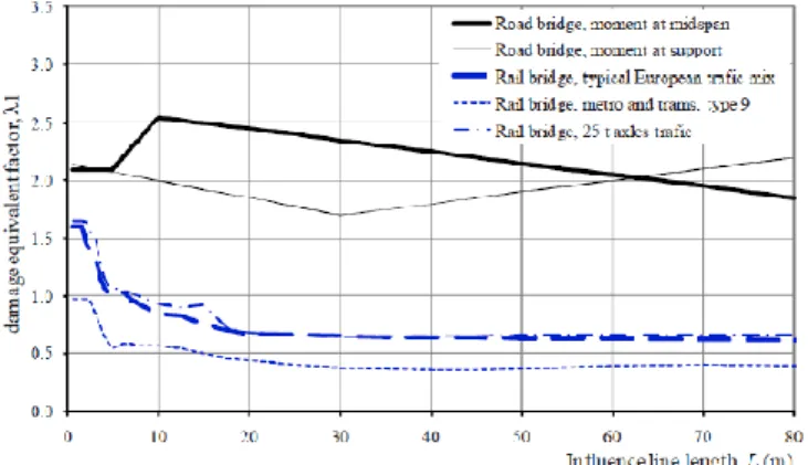
Figure 2.7: The factor λ1 for road and railway bridges as a function of the critical influence line length (Nussbaumer,

2006).

The major factors when determining the λ1 factor are the location of the studied detail to take into

account the effect of the length of the influence line/area and the type of load effect acting on this detail: bending moment or shear force. A summary of the rules in EN 1993-2, 9.5.2 when determining the λ1 factor for road bridges is given in Figure 2.8.

Figure 2.8: Damage equivalent factor λ1 for road bridge details (Al-Emrani et al., 2014).

2.3.2.2 Factor λ2

The factor λ2 is a coefficient that takes into account the annual traffic flow and the traffic composition

on the actual bridge. In bridge design, the number of heavy vehicles per year and per slow lane for road bridges (Nobs) and the amount of freight transported per track and per year for railway bridges should be

specified by a competent authority.

Factor λ2 for road bridges

According to EN 1993-2, the factor λ2 considering the actual bridge traffic flow and composition should

(24)

𝜆₂= 𝑄𝑚𝑙 𝑄₀ ∙ ( 𝑁_𝑜𝑏𝑠 𝑁₀ ) 1⁄_𝑚 (Eq. 2.19) where:

Qml is the average gross weight (kN) of the lorries in the slow lane Q0 is the equivalent weight (kN) of the reference traffic

N0 is the annual number of lorries for the reference traffic Nobs is the annual number of lorries in the slow lane

m is the slope of S-N curve; the largest m value in case of bilinear curve.

The average gross weight of the lorries in the slow lane can be calculated by the following formula:

𝑄_𝑚𝑙= (∑ 𝑛𝑖∙ 𝑄𝑖 𝑚 ∑ 𝑛𝑖 ) 1_⁄_𝑚 (Eq. 2.20) where:

ni is the number of lorries of gross weight Qi in the slow lane Qi is the gross weight of the lorry “i” in the slow lane

m is the slope of S-N curve; the largest m value in case of bilinear curve.

As stated earlier, EN 1993-2 is using the Auxerre traffic as the reference traffic data and recommends therefore using N0= 0.5E6 and Q0= 480kN when calculating the λ2 factor (for this specific case the factor λ2 is equal to 1.0). Based on these two reference values, the factor λ2 for any Qml and NObs can be obtained from Table 9.1 of EN 1993-2.

2.3.2.3 Factor λ3

The λ3 factor considers the design life of the bridge and according to EN 1993-2, this factor used for both road and railway bridges should be calculated as following:

𝜆3= (

𝑡_𝐿𝑑 100)

1_⁄_𝑚

(Eq. 2.21)

Where tLd is the design working life of the structure in years and m is the slope of the S-N curve.

The λ−coefficient method in Eurocode and the corresponding fatigue load models were derived based on a reference design life of 100 years. The λ3 factors give the possibility of modifying the design life in years as given in EN 1993-2, 9.5.2(3) and 9.5.3(6).

2.3.2.4 Factor λ4

Factor λ4 for road bridges

The factor λ4 considers the vehicles interactions and accounts the multilane effect. In other words, the λ4 factor takes into account the interactions between lorries simultaneously loading on several lanes defined in the design (multilane effect) and should be according to EN 1993-2 calculated using the following formula: 𝜆₄= √∑ 𝑁𝑗 𝑁₁∙ ( 𝜂_𝑗∙ 𝑄_𝑚𝑗 𝜂₁∙ 𝑄₁) 𝑚 𝑘 𝑗=1 𝑚 (Eq. 2.22) where:

(25)

k is the number of lanes with heavy traffic Nj is the number of lorries per year in lane j Qmj is the average gross weight of the lorries in lane j

ηj is the influence line for the internal force that produces the stress range (see Figure 2.9) m is the slope of S-N curve; the largest m value in case of bilinear curve.

This expression shows that the factor λ4 is equal to 1.0 when considering a single bridge lane.

Figure 2.9: Example of transverse distribution of two-girder bridge cross-section in function of lateral load positions (Al-Emrani et al., 2014).

2.3.2.5 Factor λmax

The final λ factor is obtained by multiplying the above mentioned individual λ−factors. An upper limit value has also to be considered defined. This is made through the factor λmax which mainly takes into

account the fatigue limit of the detail under consideration. The limitation of the damage equivalent factor value for railway bridges is based on the load model which gives an upper bound value while this factor for road bridges is on the same basis as the simulations for the λ1 factor.

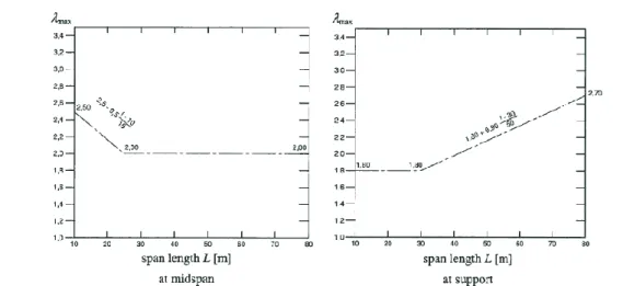
Factor λmax for road bridges

The λmax factor for road bridges for the span lengths from 10m to 80m is defined only for the sections

subjected to the fatigue stresses caused by bending moment. This is clear as the S-N curves for shear effects do not have a defined CAFL. However, when using the λ-equivalence concept FLM 3 does not generate an upper limit value to establish a suitable λmax value. The limiting λ value is therefore

established by simulating the road traffic. Similar to the λ1 factor given in EN 1993-2, the maximum λ

values are depended on the length of the bridge span and also the location of the detail under consideration. EN 1993-2 presents therefore two graphs to determine the λmax factor which are shown

in Figure 2.10.

2.3.2.6 Factor λv

For shear studs, λv,2, λv,3, λv,4 factors should be determined using the relevant equations, but using a slope coefficient m = 8, or exponent 1/8, in place of those given to allow for the relevant fatigue strength curve for headed studs in shear. Regarding λmax, the conservative values given in Figure 2.10

(26)

Figure 2.10: λmax factor for road bridge sections subjected to bending stresses (Al-Emrani et al., 2014).

2.3.2.7 Fatigue assessment on shear connectors

The shear connection fatigue assessment is based on nominal stress ranges according to EN 1994-2. In steel-concrete composite girders two different situations should be considered:

1) Where the girder top flange is always in compression (Case 2 of section 2.2.2), the fatigue assessment should be made by checking the following criterion:

𝛾_𝐹𝑓∙ ∆𝜏_𝐸,2= ∆𝜏𝐶

𝛾_{𝑀𝑓,𝑠} (Eq. 2.23)

2) Where the maximum stress in the top flange is tensile, the following interaction should be also verified (Cases 1 and 3 of section 2.2.2):

𝛾𝐹𝑓∙ ∆𝜎𝐸,2 ∆𝜎_𝐶⁄𝛾_𝑀𝑓 + 𝛾𝐹𝑓∙ ∆𝜏𝐸,2 ∆𝜏_𝐶⁄𝛾_{𝑀𝑓,𝑠}≤ 1.3 (Eq. 2.24) Also fulfilling: 𝛾_𝐹𝑓∙ ∆𝜎_𝐸,2≤ ∆𝜎𝐶 𝛾_𝑀𝑓 and 𝛾𝐹𝑓∙ ∆𝜏𝐸,2≤ ∆𝜏_𝐶 𝛾_{𝑀𝑓,𝑠} (Eq. 2.25) where:

ΔσE,2 is the normal stress range in the steel flange and γFf and γMf are the partial factors for fatigue loading and strength respectively;

ΔσC is the detail’s category;

γMf,s is the partial factor for fatigue strength for shear studs, taken with the recommended value from EN 1994-2, 2.4.1.2 (6): γMf,s = 1.0;

ΔτE,2 is the range of shear stress due to fatigue loading related to the cross-section area of the shank of the stud, determined with the uncracked properties of cross-section, even in sections considered as cracked for global analyses;

∆𝜏_𝐸,2= 𝜆_𝑣∙ Δ𝜏 (Eq. 2.26)

The maximum shear stress range Δτ is calculated according to the procedure from section 2.2.3. The expression on (Eq. 2.26) represents the range of shear stress due to fatigue loading related to the cross-section area of the shank of the stud, determined with the uncracked properties of cross-section, even in sections considered as cracked for global analyses.

(27)

2.3.2.8 Main shortcomings in the use of the damage equivalent factor method

The damage equivalence factors based on the Eurocodes presents some shortcomings, which could be summarized as follows:

 the definition of critical influence line length is non-exhaustive, and defined case by case;  the effect of simultaneity in which several trucks stand on a bridge simultaneously either in the

same lane or in several lanes is neglected;

 λ and λmax obtained for different bridge influence lines are widespread;

 the safety margin for some bridge cases are over-conservative and for some cases are non-conservative.

2.3.3 Fatigue design with the Damage Accumulation Method

Load effects generated by traffic loads on bridges are generally very complex. Not only are the stress ranges generated by these loads of variable amplitudes, but also other parameters that might affect the fatigue performance of bridge details such as the mean stress values and the sequence of loading cycles are rather stochastic.

In order to treat such complex loading situations there is a need to represent the fatigue load effects caused by the “actual” variable amplitude loading in term of equivalent constant amplitude loading. In other words, a complex loading situation such as the one shown in Figure 2.11 should be represented as one or more equivalent constant amplitude loads, so that the latter will cause equivalent fatigue damage as the real loading history. Two steps are needed:

1. Transformation of the variable amplitude loading into a representative constant amplitude loading, this is usually done by some kind of cyclic counting method.

2. Using the new set of representative constant amplitude loading to perform the fatigue design or analysis, this is done either:

 directly, by applying the Palmgren-Miner damage accumulation rule, or  by using the equivalent stress range concept.

The rules concerned with the fatigue design of bridges in Eurocode allow for the application of any of these two methods. The simplified λ-method in Eurocode is an adaption of the general equivalent stress range concept corrected by various λ-factors, while a direct application of the Palmgren-Miner rule can alternatively be used for both railway and road bridges.

Figure 2.11: An example of variable amplitude loading and stress histogram resulting from the application of cyclic counting method (Al-Emrani et al., 2014).

(28)

The most common cycle counting methods are the "rainflow" and the "reservoir" stress counting methods. In general, these two methods do not lead to exactly the same result. However, in terms of fatigue damage both counting procedures give very close results, especially for "long" stress histories.

2.3.4 Palmgren-Miner damage accumulation

As known, an S-N curve represents the relation between the stress range Δσ (or Δτ) in a specific detail and the total number of cycles to failure, N. In other words, a specific detail with a certain fatigue strength (represented by an S-N curve) will fail after N cycles of a stress range Δσ. At failure, the fatigue life is consumed and the total fatigue damage in the detail would then be 100%, or D = 1.0. If the same detail is now loaded with a number of stress cycles n < N at the same stress range, the fatigue damage accumulated in the detail would then be:

𝐷 = 𝑛 𝑁= {

1.0 𝑤ℎ𝑒𝑛 𝑛 = 𝑁

< 1.0 𝑤ℎ𝑒𝑛 𝑛 < 𝑁 (Eq. 2.27)

With this in mind, if the detail is subjected to a number i of loading blocks each with a constant amplitude stresses Δσi which is repeated ni number of times, then the total fatigue damage accumulated in the detail would be the sum of the damage caused by the individual loading blocks:

𝐷 = ∑ 𝐷𝑖 𝑖 = ∑𝑛𝑖 𝑁𝑖 𝑖 (Eq. 2.28)

2.3.5 The application of the damage accumulation method

Annex A in EN 1993-1-9 gives information on the application of the damage accumulation method in the fatigue design of steel structures. What concerns bridges the use of damage accumulation method is suggested in two cases:

1. When actual traffic data is available. This is covered in Annex B of EN 1991-2.

2. Along with the traffic load models derived for this purpose. These are LM4 for road bridges (EN 1991-2, 4.6.5) and train types 1 to 12 in Annex D of EN 1991-2 of Eurocode.

For both road and railway bridges, the traffic load models to be used with the damage accumulation method are intended to reflect the real “heavy” traffic on European road and railway networks. The variation in traffic intensity and vehicle (or train) types on individual bridges is covered by defining different “traffic types” or “traffic mixes” for road and railway traffic respectively. These are also a subject for adaption and modification by the countries through their national annexes.

In the following, the traffic load models proposed in EN 1991-2 for fatigue verification with the cumulative damage concept will be shortly introduced. A summary of the main steps involved in the application of this method is then made.

2.3.5.1 Application to road bridges

The traffic load model to be used with fatigue verification of road bridges according to the damage accumulation method is LM4. This model is composed of 5 standard lorries which are assumed to simulate the effects of real road traffic on the bridge. The definition of each lorry is given by the number of axles, the load on each axle as well as the axle spacing which are reproduced in Table 2.2. The number of heavy vehicles, Nobs per year and per slow lane (observed or estimated) applies also for fatigue verification with the damage accumulation method. Indicative figures for Nobs and the recommended values for different traffic categories are given in EN 1991-2 4.6.1(3).

(29)

The fatigue verification procedure should be performed – for those details that are determinant for the fatigue performance of the bridge – according to the following steps:

1. Establish the bridge specific data for fatigue verification. Besides the design life of the bridge this includes:

a. the “traffic category” with the associated number of heavy lorries in the slow lane, Nobs [EN 1991-2, 4.6.1(3)],

b. the “traffic type” with the associated percentage of lorries, Table 4.7 in EN 1991-2. 2. For the detail in hand, obtain the influence line for relevant load effects (shear or bending

stresses).

3. By passing the load model over the influence line, establish the time history response (i.e. stress vs. time, or time step)

4. Construct the stress histogram by mean of a cycle-counting method.

5. Select an appropriate fatigue category and establish the corresponding S-N curve (ΔσC at 2E6 cycles, ΔσD at 5E6 cycles and ΔσL at 100E6 cycles).

6. Use the stress histogram either to: a. Calculate a total damage:

𝐷_𝑖= { 𝑛_𝑖 5𝐸6∙ ( 𝛾𝐹𝑓∙ 𝛾𝑀𝑓∙ ∆𝜎𝑖 ∆𝜎𝐷 ) 3 𝑖𝑓 𝛾_𝐹𝑓∙ ∆𝜎_𝑖≥∆𝜎𝐷 𝛾𝑀𝑓 𝑛𝑖 5𝐸6∙ ( 𝛾_𝐹𝑓∙ 𝛾_𝑀𝑓∙ ∆𝜎_𝑖 ∆𝜎𝐷 ) 5 𝑖𝑓 ∆𝜎𝐿 𝛾𝑀𝑓 ≤ 𝛾𝐹𝑓∙ ∆𝜎𝑖< ∆𝜎𝐷 𝛾𝑀𝑓 (Eq. 2.29)

and verify that:

𝐷 = ∑ 𝐷𝑖 𝑖

≤ 1.0 _{(Eq. 2.30)}

b. Calculate the equivalent stress at 2E6 cycles:

∆𝜎𝐸= ( ∑ 𝑛𝑖∙ (𝛾𝐹𝑓∙ ∆𝜎𝑖) 3 + ∑ 𝑛𝑗∙ (𝛾𝐹𝑓∙ ∆𝜎𝑗) 3 ∙ (𝛾𝐹𝑓∙ 𝛾_∆𝜎𝑀𝑓∙ ∆𝜎𝑗 𝐷 ) 2 ∑ 𝑛𝑖+ ∑ 𝑛𝑗 ) 1 3 ⁄ (Eq. 2.31) from (Eq. 2.15): ∆𝜎_𝐸,2= ∆𝜎_𝐸∙ ( 𝑁 2𝐸6) 1 3 ⁄ (Eq. 2.32)

and verify that:

∆𝜎_𝐸,2∙ 𝛾_𝐹𝑓∙ 𝛾_𝑀𝑓

∆𝜎_𝐶 ≤ 1.0 (Eq. 2.33)

(30)

Figure 2.12: The application steps of cumulative damage method (Al-Emrani et al., 2014).

2.3.6 Fatigue strength

2.3.6.1 Set of fatigue strength curves (EN 1993-1-9)

The statistical analysis of the test results on a specific structural detail allows for the definition of one fatigue strength curve. Numerous fatigue tests programs on different details in steel have shown that the fatigue strength curves are more or less parallel. Fatigue strength is thus only a function of the constant C, see (Eq. 2.34), which value is specific to each structural detail.

𝑙𝑜𝑔𝑁 = 𝑙𝑜𝑔𝐶 − 𝑚 ∙ log (∆𝜎) (Eq. 2.34)

Since there are many different details, so is the number of the different strength curves, and this is unusable for design in practice. The solution is the classification of the different structural details in categories with a corresponding set of fatigue strength curves.

Classified structural details may be described in different EN 1993 associated Eurocodes (EN 1993-1-9, EN 1993-2, EN 1993-3-2, etc.) but they all refer to the same set of fatigue strength curves, as given in the

(31)

generic part 1-9. Each detail category corresponds to one S-N curve where the fatigue strength Δσ is a function of the number of cycles, N, both represented in logarithmic scale. The set is composed of 14 S-N curves, equally spaced in log scale. The set has been kept the same over the last decades; it comes from the ECCS original work of drafting the first European recommendations (ECCS, 1985). The set is reproduced in Figure 2.13.

Figure 2.13: Set of fatigue strength (S-N) curves for normal stress ranges (Nussbaumer et al., 2011).

The spacing between curves corresponds to a difference in stress range of about 12% (values corresponding to the detail categories were rounded off), i.e. 1/20 of an order of magnitude on the stress range scale. All curves composing the set are parallel and each curve is characterized, by convention, by the detail category, ΔσC (value of the fatigue strength at 2 million cycles, expressed in N/mm2). It is also characterized by the constant amplitude fatigue limit (CAFL), ΔσD, at 5 million cycles, which represents about 74% of ΔσC. The slope coefficient m is equal to 3 for lives shorter than 5 million

cycles. For constant amplitude stress ranges equal to or below the CAFL, the fatigue life is infinite. The CAFL is fixed at 5 million cycles for all detail categories. This is not exactly the case in real fatigue behaviour but has advantages for damage sum computations. Other codes use different values.

Under variable amplitude loadings, the CAFL does not exist, but still has an influence. Thus, a change in the slope coefficient is made, the value m = 5 being used between 5 million and 100 million of cycles. This last value corresponds to the cut-off limit, ΔσL, which corresponds to about 40% of ΔσC. By

definition, all cycles with stress ranges equal to or below ΔσL can be neglected when performing a

damage sum. The reason for this is that the contribution of these stress ranges to the total damage is considered as being negligible. It should be emphasised that the double slope S-N curve (and the cut-off limit), compared to the unique slope curve, represents better the damaging process due to cycles below the CAFL.

If a structural detail configuration from a type of structure can be found in the tables of the relevant EN 1993 associated Eurocodes, and the description and requirements for this detail correspond, then the fatigue strength can be derived from the standard fatigue resistance S-N curves given in EN 1993, generic part 1-9.