OpenCommons@UConn
Doctoral Dissertations
University of Connecticut Graduate School
5-4-2015
Classification and Multiple Hypothesis Testing in
Microarray and RNA-Seq Experiments
Patrick B. Harrington
University of Connecticut - Storrs, [email protected]
Follow this and additional works at:
https://opencommons.uconn.edu/dissertations
Recommended Citation
Harrington, Patrick B., "Classification and Multiple Hypothesis Testing in Microarray and RNA-Seq Experiments" (2015).Doctoral Dissertations. 748.
Experiments
Patrick Harrington, Ph.D. University of Connecticut, 2015
This thesis focuses on analyzing the type of data returned by two pieces of technology, the older and less expensive microarray, or the next generation sequencing data, RNA-Seq. Both devices return data that is extremely large in volume. Microarray analysis begins by finding genes of interest, which are called differentially expressed (DE). Genes are called DE controlling for some criteria, such as false discovery rate (FDR), and then clustered into groups. A method unifying these two steps was suggested, using a mixture of normal distributions with the appropriate EM algorithm. We compare this to a semi-parametric alternative to the unified method. We use simulation studies to compare these and other microarray analysis methods. We then look at next generation RNA-Seq data, with a focus on accounting for gene length. We introduce a hierarchical, log-linear negative binomial count model which incorporates gene length both into the parameter estimation and zero count inflation for this data. This hierarchical model allows borrowing counts information across genes efficiently and provides a Bayes factor criterion for screening for DE genes.We use real data to show a decrease in length bias when our method is compared to popular existing methods, as well as a simulation study to establish the effects of over and under fitting within our model, as well as the effect of fitting multiple DE types in a single model. We provide new methods for finding DE genes for microarray and RNA-Seq data, and illustrate their advantages using real and simulated data.
Experiments
Patrick Harrington
B.S., California Polytchnic State University, San Luis Obispo, California, 2007
A Dissertation
Submitted in Partial Fulfillment of the Requirements for the Degree of
Doctor of Philosophy at the
University of Connecticut 2015
Patrick Harrington
Doctor of Philosophy Dissertation
Classification and Multiple Hypothesis Testing in Microarray and RNA-Seq Experiments Presented by Patrick Harrington, B.S. Major Advisor Lynn Kuo Associate Advisor Ming-Hui Chen Associate Advisor Zhiyi Chi University of Connecticut 2015 ii
Harrington
supportive and loving than my parents, sister, and newborn. I would like to acknowledge each and every person who has helped me along my path to and beyond this current state, for the way in which they have helped me. Specifically, there are a handful of people to whom I am extremely indebted. I would like to thank Ming-Hui Chen for all of his help in so many different aspects of my studies. Beyond giving me enormous support throughout my entire time at UConn, he gave me attention and knowledge through the classes he taught me, the input he gave me on research, and consulting as well. Zhiyi Chi also gave me much support and help in classes, as well as great advice and direction outside of the classroom. Along with my advisor, these Professors have shown an amazing amount of patience and support, and been very accommodating. Without such great efforts, it is hard to imagine having made it through this program. And of course, by far the largest appreciation goes to my advisor, Lynn Kuo. The countless hours of support and help she has given me were absolutely the foundation on which this work is built. I know she must have endless support and patience, since she gave those to me. Without her direction and expertise in the areas of my thesis work, I would have been completely lost. Kind words could never properly express my feelings, and I hope my never ending gratitude will.
Chapter 1: Introduction 1 Chapter 2: Microarray 17 2.1 Data . . . 21 2.2 Assumption . . . 22 2.3 Inference . . . 23 2.3.1 Density Estimation . . . 23 2.3.2 Semi-Parameteric . . . 25
2.3.2.1 Overview Of SOM Algorithm . . . 25
2.3.2.2 SOM In Microarray . . . 27
2.3.2.3 Grow Step . . . 28
2.3.2.4 Smooth Step . . . 32
2.3.2.5 Density Estimator Using SOM . . . 36
2.3.2.6 Clustering . . . 37
2.3.2.7 Optimal Cluster Identification . . . 40
2.3.2.8 SOM: Non-Parametric DE Classification . . . 44
2.3.2.9 SOM: Semi-Parametric DE Classification . . . 45
2.3.3 Parametric . . . 46
2.3.3.1 Initializing EM With SOM . . . 46
2.3.3.2 Expectation Maximization . . . 48
2.3.3.3 Rejection Rule . . . 48
2.4 Interpretation . . . 49
2.4.1 Results . . . 50
2.4.3 Non-Traditional Mixtures . . . 52
2.5 Conclusions. . . 56
Chapter 3: RNA-Seq 58 3.1 Data . . . 63
3.2 Negative Binomial Model . . . 64
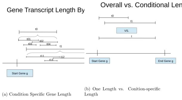
3.3 Transcript Length . . . 66
3.3.1 Zero Counts . . . 67
3.4 Hierarchical log-linear Model . . . 71
3.4.1 Likelihoods . . . 75 3.4.2 Prior Choices . . . 75 3.4.3 Posterior Inference . . . 76 3.4.3.1 Base 1 . . . 77 3.4.3.2 Base 2 . . . 79 3.4.3.3 Intercept-Shift . . . 79 3.4.3.4 Condition-Specific . . . 81 3.4.3.5 Slope-Shift . . . 83 3.4.3.6 Intercept-Condition . . . 86 3.4.3.7 Intercept-Slope . . . 89 3.4.4 Hyper Parameters . . . 92 3.5 Model Assessment . . . 94 3.6 Results . . . 96 3.6.1 Simulation Study . . . 96 vi
3.6.2.1 Comparing New Methods With Existing Methods . . . 100 3.7 Conclusion . . . 103 3.8 Future Work . . . 105
Chapter 4: Conclusion 107
1 Sampling Distributions For Mixture of Normal Distriubtions. . . 50 2 Error rate comparisons among seven methods from simulation study 1 . . . 51 3 Error rate comparisons among seven methods from simulation study 2 . . . 55 4 AUC comparison for over fitting, under fitting, and properly fitting the
overdispersion parameter . . . 97 5 AUC comparison for over fitting, under fitting, and properly fitting the
intercept term . . . 98 6 Results: DIC, dimensional penalty and LPML for Models: Forβ2, library
size coefficient is shared across all genes . . . 99 7 Intersection of top 500 genes existing methods. . . 101 8 Intersection of top 500 genes our models with summary of existing methods. . . . 102 9 Intersection of top 500 genes our models with existing methods . . . 102
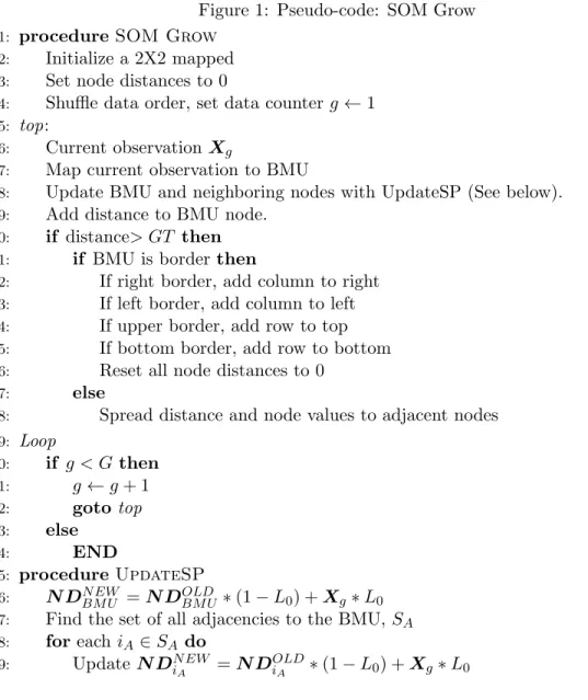
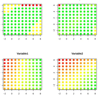
1 Pseudo-code: SOM Grow . . . 30 2 SOM output by variable:Initial graph after grow and before smooth steps.
Each Plot represents a variable. Each dot inside of the plots corresponds to a node location in the map space. The colors represent the value for the variable at the node. Green values are smaller and red values are larger . . 31 3 Pseudo-code: SOM Smooth . . . 34 4 SOM output by Variable: Initial graph after the smooth step. Each Plot
represents a variable. Each dot inside of the plots corresponds to a node location in the map space. The colors represent the value for the variable at the node. Green values are smaller and red values are larger . . . 35 5 Pseudo-code: SOMWard . . . 39 6 SOM output:Full output including clustering and frequency. SOMWard
Clusters shows cluster by color, frequency shows frequency, and variable 1 and 2 are the variables from the data. . . 39 7 Pseudo-code: CAN . . . 41 8 Distances (log distances) for the joined clusters versus the number of clusters 42 9 Differences of the distances (log distances) for the joined clusters versus the
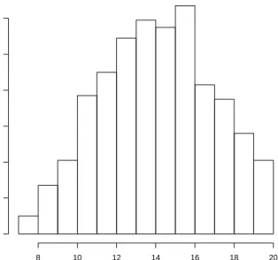
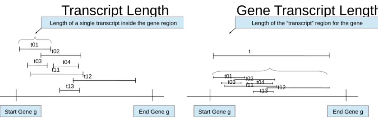
number of clusters . . . 42 10 Distances and Distance Jumps for Ward Alternative . . . 44 11 Histogram of Optimal Cluster Numbers Chosen By BIC For Example 1 . . 53 12 Plot of data from example 1 . . . 55 13 Transcript Lengths . . . 67
15 Zero Counts by length and coverage . . . 70
16 Zero Count By Length: Proportion of zero counts by gene length. Overlay estimated probability of zero count in red. . . 71
17 Transcript Assembly and Pre-Processing . . . 72
18 Graphical Model Intercept Shift Model. . . 74
19 Metropolis-Hastings:Updatingθ . . . 77
20 Comparison of ROC curves . . . 99
21 Plot of average lengths comparison of top selected genes among our three models and EdgeR . . . 103
Introduction
Genomic studies aim to understand the role genes play in our everyday lives. This involves numerous mappings of the human genome, numerous mappings of the genomes of other animals, and studies identifying the functionality of genes. Advances in technology and methodology have made genomic studies possible, and greatly increased the efficiency of such studies. One of the earlier, and still very popular pieces of technology is the microarray. Another popular, newer, and more expensive technology is based in RNA-Seq data, such as 454. In this thesis, we will cover methods currently used in the analysis of both microarray and RNA-Seq data.
In microarray experiments, the researcher typically has a pair of conditions, control and treatment, or a number of conditions, control, treatment 1, treatment 2, and so on for some number of treatments. The manner in which data is collected allows for the analysis of pairwise comparisons (i.e. difference in gene expression from one condition to another). In many cases where scientists develop and test a hypothesis, they know exactly what they are looking for. An example of this in the genomic setting would be the belief that a specific gene was involved in a specific process (like bone growth). There are also cases
in which we don’t have such a clear idea of what to expect. An example of this would be the desire to see which of a large group of genes are involved in certain processes.
Microarray experiments can be used for both of these types of hypotheses. Microarray experiments are run using a piece of technology that has a lattice of addresses. Each well is treated with a solution that is comprised of genetic material. We usually associate that genetic material with exactly one gene. Multiple addresses from any one microarray have material representing the same gene, but cannot have material from more than a single gene. It is conventional to think of each well as a probe, typically given some identifier (Probe ID). This Probe ID is usually given by the software used for collecting and analyzing data, or the scientists running the experiment. Each Probe ID is linked to some official gene.
Within each microarray, the probes are put in the same order. While the conclusions from a microarray experiment are made with respect to the genes each probe represents, the actual analysis is run per probe. This means that the probes must be linked from microarray to microarray. This could mean using the exact same probe to well layout in each microarray, or simply tracking the manner in which this is permuted. Also, this means that the exact same probes must be placed on every single microarray.
In order to prepare a microarray, the genetic material needed for each probe is treated with the appropriate condition. There is often a control case, in which no treatment is made, although experiments can be run with a number of conditions all of which involve some treatment. In order to get gene expression (by probe), a measure that quantifies how much of a gene is present in certain conditions, a visual read is made on each well. In order for such a read to be possible, it is needed to introduce some dye. The reads themselves are made by machines. In order to account for various types of dependencies
and errors within these machine reads, the scientist makes both a background read and an actual read for each probe.
This requires two dyes, the most popular choices of which are Cy3 and Cy5. In order for a biological treatment to be prepared for each well, there is a treatment and quality control step that are performed. After this, the dye is applied. When getting gene expressions for each probe, the background dye and other dye are scanned in separately. The background read represents a baseline read for each probe. The other read represents the abundance of that specific gene within each treatment. The ratio (or logged ratio) of these reads is the quantitative value associated with each probe, typically referred to as gene expression. In order to avoid poor reads, multiple reads are taken for both dyes for each probe. One value, such as the median of all such reads, is recorded for each dye in each probe. Another way to avoid (or account) for technical error is to flag probes for which the device believes there was a bad read. Before the data is analyzed, more pre-processing is done to identify which probes have bad readings in which arrays. This leads to a smaller number of probes being analyzed than are present in the microarrays. Another step that is taken to reduce error in the experiment is dye swap. The two dyes used can have different potencies, or other differences we attribute to dye effect. In order to capture this effect, the scientist can use a technique called dye swap. Here, the scientist runs a number of replicates for each condition, with some dedicated to one dye combination, and the others swapping the dye combination. This allows for both the estimation and incorporation of the dye effect.
Once each probe for each microarray has a quantitative value, gene expression, and once all needed preprocessing has been made, the goal of the analysis is to identify genes which act differently across the conditions. We call these genes differentially expressed
(DE), the alternative to the null classification of equivalently expressed (EE) genes. This thesis focuses on microarray experiments in which a group of genes are first to be classified as EE or DE, and then to be further clustered based on the expression data.
Microarrays have thousands and thousands of addresses. This combines with the flexibility of the device to allow the scientist to test thousands of genes simultaneously. It is possible (and conventional) to have multiple probes on each device dedicated to a single gene. It is possible to include genes which should show no change in expression across the conditions of interest. These serve as control genes, allowing the scientist to validate the results of the experiment.
When choosing which genes to include in the study, it is conventional to not only include genes that are expected to be involved in the processes being tested (i.e. acting differently in the treatment condition than the control), but also to include genes that are not expected to be involved in the process. This serves as a validation for the overall conclusion of the experiment.
There have been many methodologies suggested for finding DE genes in the microarray setting, a few of which are covered in this thesis. One popular approach, a linear modeling approach incorporating a Bayesian technique for borrowing across the genes, LIMMA (Smyth (2004)). Another very popular approach, Significance Analysis of Microarrays (SAM), was introduced in Tusher et al. (2001). This is a non-parametric alternative. Both of these methods give the user the ability to rank the genes with respect to their likelihoods of being DE, as well as offering p-values. Further, these methods allow the scientist to control for a predefined false discovery rate (FDR). Should the analyst use either of these, or any of the other methods for finding a set of DE genes, the next step is to try to find groupings within this set of DE genes.
This fits into clustering, or cluster analysis. Traditionally, cluster analysis is based on a distance metric. In this setting, the goal is to identify groups of like genes. The same expression data used to call genes DE is used to classify them. Clustering algorithms can be broken down into hierarchical and non-hierarchical. Hierarchical algorithms are either agglomerative, which initially considers every observation its own cluster and joins them together, or divisive, in which a single cluster is broken into many. A criterion, such as matched distances or a function thereof, can be recorded for each of the joining or dividing steps. Then, the number of clusters maximizing that criterion is chosen to be the best. Other very popular methods include k-means MacQueen (1967), partitioning around the mediod (PAM) Kaufman and Rousseeuw (1987), and EM algorithms Hartley (1958)based on some mixture distribution assumption.
One popular non-parametric clustering algorithm was developed in Kohonen (1982). The self organizing map (SOM) uses two spaces, a map space which is a topological graph, and the data space. In most cases, the data space is an m dimensional real space with Euclidean distance. The map is comprised of a lattice of nodes, the number of connections for each node is determined by the topology. Popular topologies include rectangular, with 4 adjacencies per node, and hexagonal, with 6 adjacencies per node. There is a separate distance function for the map space and the data space, although it is common to use euclidean distance for both. Each node in the map represents a vector in the data space. This vector is similar to the location of the node in the data space. The map needs to be initialized, by either setting the initial dimensions or growing the map, and then the map is smoothed. The smoothing step involves updating the map with the data in order to make the nodes of the map fit the data. The map can be further smoothed by using a neighborhood function. A neighborhood function (NF) is based on the distance function
in the map space, and assigns weights between two nodes, where the weight is decreasing in the distance. The NF is used to control how much smoothing occurs when training the map. One popular smoothing algorithm is called a batch algorithm. It updates each node based on the entire training dataset, as a batch. It converges quickly with respect to computational time, and based on an initial map, converges to a deterministic map.
It can be noticed that a set of assumptions is used to find DE genes. Then, another method, usually with its own set of assumptions, is used to cluster the DE genes into groups. That is why Yuan and Kendziorski (2006) actually integrated the two goals with one method, which they call the Unified Method. They state the methodology broadly. It is based on any mixture distribution assumption, where one of the mixands is set to be for the equivalently expressed genes. They develop machinery for ranking genes in being DE, as well as a method for estimating and controlling FDR. The paper then focuses on a mixture of normals assumption, where all of the parameters including the true number of mixands must be estimated. An EM algorithm is used to classify the genes. The approach suggests fitting an EM algorithm for cluster number ranging from 2 to some top value, and then some criterion such as AIC or BIC can be used to determine the true number of clusters.
We address some of the issues that can come with using an EM algorithm. It can be very computationally expensive to look at the results for the EM algorithm for clusters from 2 to some top value, especially when the true number of clusters is large. Also, the convergence of the algorithm isn’t ensured in cases where the model is mis-specified, including when the true number of clusters is mis-specified. This means that whichever criterion is used to determine the true number of clusters can’t be relied on unless the true number of clusters is specified. Even if the criterion has a good interpretation for
the mis-specified model, there isn’t any assurance the values of the criterion are based on convergent states. It is completely possible for the criterion chosen to achieve a local maximum with respect to the criterion before the number of clusters considered is even close to the true number of clusters, and even if the true number of clusters is identified, it could take an enormous amount of computing resources to identify it. We address these issues using a specific application of SOM.
We use a growing SOM, with a batch smoothing algorithm to train a map with di-mension determined by the data. We use a variant of a popular hierarchical clustering algorithm to join our map into regions, or clusters, based on Euclidean distance metrics in both the data and map spaces. We establish a methodology to find the true number of clusters based on the hierarchical results. We then use a similar method to rank the true number of clusters by our criterion, which can return a limited list of possible cluster numbers to try in the case of fitting an EM algorithm. We also save the initial states for each cluster in our results, and use them to initialize the EM algorithm, which leads to faster and more reliable results. This directly addresses the issues of the EM algorithm.
We then extend this method to classify DE genes. One problem with using a mixture distribution assumption is that each mixand must be focused on and estimated. In order to get reasonable estimates, sometimes the structure of the mixture must be overly restrictive. Also, some type of EM or some equivalent is needed to arrive at a solution. While some of the concerns for the EM have already been addressed, it would be nice to develop a mixture distribution that is less restrictive than more traditional methods, and has some methodology to call genes DE. With this in mind we develop a non-parametric approach for DE gene classification based on the SOM map. A truly non-parametric approach is
considered nice since it doesn’t have restrictive assumptions, but especially for something as complex as classification, it can be difficult to estimate how well your classification is.
Due to this, we use one basic assumption on the mixture distribution. We assume that the null cluster, that is all the genes which are equivalently expressed, have changes from control to treatment centered at a change vector of zero, with a normal shape. We do not put any extra assumptions on DE portion of the data. In fact, one integral part of this is estimating the multivariate pdf of the data, which we accomplish within the SOM framework. This estimate allows us to ignore the form of the rest of the mixture distribution. The assumption put on the null cluster of genes is intuitive as it fits our notion of what an EE gene does (noise randomly placed around no change). We introduce an alternative to the original clustering approach which doesn’t help to find the number of clusters in the data, or provide initial estimates for the EM algorithm, but instead focuses on joining nodes to the null cluster. A rule for when to stop joining nodes to the null cluster is used, and then the probability that a gene is EE given the data is estimated. These estimates are used to rank genes as DE, estimate the false discovery rate of a group of genes called DE, and control for a false discovery rate. LIMMA, SAM, the Unified Method, and our SOM methodology are compared in a number of specific setting using simulation studies. While our SOM methodology is outperformed by the existing methods when measured from false discovery rate (FDR), false non discover rate (FNDR), empirical type 1 and type2 errors, these situations are from the mixture of normal assumption that is most appropriate for all the methods. We then go through a number of examples of data simulated from mixtures which the mixture of normals EM algorithm is not expected to do well. We look at the same measures to see how successful our methodology performs.
Since the introduction of microarray technology, many advances have been made in the area of genomic studies. We turn our focus to next generation sequencing (NGS), which is considered second gneration RNA-Seq. RNA-Seq data is fairly new. Before any data can be collected, biological specimens are treated with a condition, sampled, and the RNA is sequenced. This process includes isolating RNA from the cells, fragmenting the RNA, copying the RNA into cDNA, and amplifying the fragments. Once these biological steps are completed, the data is sequenced into reads. These reads are strands of the RNA, and raw data has a form with sequence name, corresponding read, and in some cases a quality score for the read. There are a number of new devices being developed which return this type of data, with formats varying more so than with the somewhat standard microarray. Each device used to gather RNA-Seq data has a number of lanes. Each lane can be thought of as being similar to a microarray. That is, each lane can be given biological samples that have been treated differently (i.e. each lane corresponds to its own condition), each lane can be given replicates from samples treated identically (i.e. each lane corresponds to a replicate), lanes can be given a replicate within a condition, and so on.
The main difference in the preparation and resulting expression for each biological sam-ple is in how counts are separated for genes. Like in microarray experiments, RNA-Seq experiments begin with biological samples gathered in different conditions. Unlike mi-croarray experiments, the specific genes to be studied are not determined by the scientist, but instead the experiment. There are no addresses that get filled with a solution com-prised of genetic material for a specific gene. Instead, each lane receives genetic material corresponding to all genes represented inside of the biological sample. This specifically rules out the ability to use null genes as validation for the results of the experiment.
Further, this limits a scientist’s ability to focus on specific genes within a hypothesis. Transcriptome is defined as the set of all RNA within a cell at a given time. For each living thing, this changes over time. So technically the genes found within an experiment based on cells from a single living creature will change over time, meaning that two runs of the same experiment on a single organism could yield a different set of genes. However, one would expect for the trasncriptome analysis to yield similar results from run to run.
Instead of reading expression levels as illumination reads from individual addresses, each lane of biological material returns reads. These reads are RNA Sequences of a certain length. Depending on the technology being used, these reads can be of fixed or random length, and these lengths can be long or short. Length is measured in base pairs, and counts the number of nucleotide base pairs (typically represented by letters) in a read of RNA. An RNA-Seq experiment returns what is called a sequence library. This collection of all reads from a device is considered to be a snapshot in time of the trasncriptome of the biological sample. For properly executed experiments, the differences in these libraries from transcriptome to transcriptome are attributed to the difference in condition from collection of transcriptome to transcriptome. So, much like a scientist would look to quantify changes in gene expression in the microarray setting in order to identify genes which act differently across a set of conditions, one would look for differences in these libraries for RNA-Seq experiments. Unlike the microarray where each gene is identified via the Probe IDs for each well, the RNA-Seq data simply has a bunch of reads which can be mapped to the genome. The first level of difficulty is mapping each read to the desired genome and arriving at what is considered the raw data.
The typical steps for taking data from the reads making up a sequence library into raw count data is to assemble transcripts. Transcript assembly is usually taken care of by
aligning large sets of short reads to a genome. A very popular method for this is Bowtie (Langmead et al. (2009)). The goal of Bowtie is to take a large number of these shorter reads and align them with the genome. In order to understand how this is done, it is important to understand how the reads are made. The genetic material for any lane is sequenced. This involves reading the sequencing, which is typically done one nucleotide at a time. There are possible errors here, including reading a nucleotide which isn’t actually there, reading a single nucleotide multiple times, and skipping nucleotides which are there. The result is always a read of nucleotides, so there isn’t always a way to know the chance that any given read has any of these possible errors in it. When matching reads to the genome, the problem is in part allowing for these types of errors to be present in our reads while still mapping them to the genome. Another difficulty comes from the possibility of multiple matches. The shorter a read, the larger the expected number of matches. One way to minimize this problem is to use longer reads, but due to monetary restrictions and technological limitations, this may not always be a possible solution. Bowtie is constructed to deal with short reads, and is ultrafast and memory efficient. Bowtie is not a final step, but its output is used by other processing tools.
One such tool is Tophat. Tophat (Trapnell et al. (2009)) was developed to build on Bowtie. Bowtie relies on known splice junctions. Tophat doesn’t need these predetermined splice junctions, and instead can find novel splice junctions based on the data. When introduced, this method had great results in finding both previously known splice junctions as well as a large number of novel ones. Additionally, the steps can be run at a very high level of efficiency. When completed, tophat returns some reads that can be mapped to the genome, and others which cannot. MapSplice (Wang et al. (2010)) was introduced as
an extension to Tophat. It focuses on high accuracy (sensitivity and specificity) in the detection of splice junctions and computational efficiency.
Tophat remains quite popular for a number of reasons. One of these is that the output from tophat can be taken directly in by Cuff Links. Cuff Links is a part of a system created for the purpose of analyzing RNA-Seq data. Trapnell et al. (2010) introduced Cuff Links to build on the tophat method. It can take the alignments output by Tophat, and assemble them into transcripts. Transcripts are assembled reads. These reads are mapped over the same region of the genome. For each transcript, we can track the number of reads mapped to that transcript, and the length of the transcript in addition to the location of the transcript on the genome. It is important to notice that reads can be aligned to multiple locations on the genome. This means that reads can be mapped to multiple transcripts. Since the goal of running the experiment is to eventually analyze multiple libraries, it is important to get count data from these raw reads. This requires estimating counts for each of these transcripts. These estimated counts and lengths are returned by Cuff Links. It should be noted that these estimated counts are not actually counts, and depending on how the data is to be analyzed, some rule for converting them into counts may need to be used. Once the data has been processed by tophat, and then by Cuff Links, the current state of the data is to have mapped reads to the genome, and then to transcripts. The next step is to take the transcripts and map them to regions in the genome. This is again done by Cuff Links. When this step has been completed, the output still isn’t in the form needed for analysis. One file should be used to describe each lane of the device. These files have a number of transcripts, described by estimated count and overall transcript length. The analyst must at this point combine all transcripts within each lane into a single count and length estimate for each gene. It should be noted that
bar codes, or identifiable RNA sequences, can be placed on reads from different biological samples in cases where the scientist wishes to use a complex design for the experiment. This would allow for multiple values to be tracked per gene, breaking each estimated count and length down by bar code. For this thesis, we didn’t explore any data of this type, but the processing requires just one more step to get the count data needed to analyze the experiment. Of course, this more complex setting will require more complex methods of analysis. The final processed form of the data is arrived at by joining these files for each lane together. The result is a single dataset.
The union of all of the genes for each lane make up the list of all genes represented in the study. The final dataset has one row for each of these genes. Genes which are in this list need not be present in every lane. Each gene in the dataset has a value for gene length in each lane, and estimated count in each lane. For lanes in which a gene is not present, the value of 0 is recorded for both length and estimated count. This is typically referred to as the raw data for any RNA-Seq experiment. Before analysis, however, many scientists will choose to use one more processing step. This is to identify genes which are not present in many of the lanes. The idea here is that Bowtie and Tophat could well improperly assign reads to portions of the genome. This leads to genes not present in the study to be observed in the sequenced results, although not necessarily in every lane. Genes which are not present in the study while being observed in the sequenced lanes tend to be present in a smaller number of lanes than any of the genes actually present in the study. The scientist analyzing the data must create a rule for omitting genes from this final list which are likely present only due to technical error. The conventional approach is to omit genes for which there are a large number of zero counts, since that is equivalent to not being present in a large number of the lanes. It is with this description in mind
that some methods for analyzing this data use special consideration for zero counts, as does the methodology we suggest.
For RNA-Seq, the steps of aligning reads to a genome, assembling those reads into transcripts, and mapping those transcripts to a reference genome need not be accomplished using the specific methods listed here. We specify the methods used by us in preparing our read data for analysis, but others have used entirely different methods for each of the steps. Should a scientist wish to analyze RNA-Seq data, however, these steps will need to be accomplished with some method. One reason these specific steps were chosen is that they are all made available through psu.galaxy.org (Goecks et al. (2010), Blankenberg et al. (2010), Giardine et al. (2005)). In fact, for many steps needed to simply get the data in the proper format for different tools and many extensions to steps taken in this paper can be found on galaxy. It offers comprehensive documentation and a relatively friendly community to ask questions and collaborate with. Beyond being free to use and offering a large amount of storage on a cloud computing foundation, galaxy offers the user a single place and tool to perform each step and pass the data along carefully constructed work flows.
With the raw count data in hand, there are a number of methods which can be used to analyze the data. Out data falls into a control, or treatment case. The methodology we list here considers that case as well. Count data assumptions typically use a Poisson, binomial, or a negative binomial distribution to model the data. Such methods include EdgeR (Smyth and Robinson (2007b), Smyth and Robinson (2007a)) and DESeq (Anders and Huber (2010)). In (Smyth and Robinson (2007b)) Smyth covers the approaches to analysis predating his. Of all the distributional assumptions, his works is based on the negative binomial model. He uses a parameterization that allows for a mean and
overdispersion parameter. He noticed that the total count of reads per lane, which he calls library size, differs. The differences in counts from lane to lane could be due to the library size, as opposed to condition. To that end, he allowed the mean for each gene in a given lane to be proportional to the library size, and said that there was a condition specific rate. The null vs alternative hypothesis for each gene in this setting is equivalent to testing to see if the control rate is equal to the treatment rate. In this methodology, a Wald type statistic is created by estimating the true control and treatment rates, and the variance of those estimates. In cases where the sample size is too small to warrant using the Wald type statistic, an exact test is available.
Length bias in large part motivated the RNA-Seq work in this paper. It has been noted empirically that in general, there is a positive relationship between the length of a gene and the chance that gene is called DE. We explore gene length in depth. We look at the current way of calculating gene length, and suggest a different consideration, a condition-specific gene length. This consideration is motivated by an explanation for why genes with a longer length is more likely to be called DE. Our belief is that there are a group of genes which have different regions activated from control to treatment. This would mean that transcripts from the control setting are mapped to different regions of a gene than those from the treatment setting. One way to conclude that transcripts for a gene are mapped to different regions of the genome in different settings is to notice that they have significantly different gene lengths. Instead of simply trying to find genes with different condition-specific lengths, we find genes where the change in observed values can be explained by the different specific lengths. In addition to modeling condition-specific gene length, we incorporate gene length into our model, while also accounting for library size. We introduce a hierarchical linear modeling approach for estimating the log
of the true mean counts for a gene in a given lane, equipped with a method for calling genes DE. Our approach also uses an intuitive approach for accounting for zero counts which is also based on the gene length. This method is flexible enough to identify 3 different types of differentially expressed genes, and the results of applying it to real data are compared with EdgeR to show a reduction in length bias. We also use a simulation study to further understand the possible effects of over/under fitting, as well as to see if there are multicollinearity concerns with fitting more than one type of DE gene in a model.
As a general note, we refer to simulation studies for both the microarray and RNA-Seq sections of this thesis. Part of the computation was done on the Beowulf cluster of the Department of Statistics, University of Connecticut, partially financed by the NSF SCREMS (Scientific Computing Research Environments for the Mathematical Sciences) grant number 0723557.
Microarray
Microarrays give us the ability to observe the expression levels of tens of thousands of genes simultaneously in both treatment and control scenarios. Further, they can be used to see how gene expression levels change over time. This allows us to explore large groups of genes of interest, both for known and unknown biological properties. In order to find genes of interest within the group of genes studied, the first step is typically to identify differentially expressed (DE) genes. These genes are found using some assumptions on the numeric values representing their expression levels at each treatment level considered. One very popular method for finding DE genes is Linear Models for Microarrays (LIMMA) as presented by Smyth (2004). In this method, linear modeling is utilized along with a set of prior distributions for the regression coefficients and variance. Another popular method is Significance Analysis of Microarrays (SAM), as presented by Tusher et al. (2001). This method doesn’t rely on the parametric assumptions as in the case of LIMMA. Instead, it finds a gene specific t-statistic using a gene specific standard deviation and a common standard deviation correction. Based on these values, a group of potentially differentially expresse genes are identified. SAM focuses on controlling a false discovery rate (FDR),
and uses permutations of the measurements to assess the FDR of the group of genes. However, in cases where parametric assumptions are approximately true, this method will be outperformed by some methods with appropriate assumptions.
While originally designed to simply find DE genes without considering time course data, both of the above methods have been adapted and are used in time course settings. We wish to consider methods created for the sole purpose of time course. Tai and Speed (2006) offer a Multivariate Emprical Bayes Statistic (MB-statistic) for ranking genes in a time course setting. We will outline how to deal with this later.
While the previous papers talk about methods for identifying genes which are differ-entially expressed, none have addressed the issue of identifying a latent structure where similar genes have similar expressions. In many, if not all microarray experiments, af-ter identifying the DE genes, the scientists perform some clusaf-tering method. The idea being that they can find genes which have similar behavior and characteristics based on similarities in their expressions. Whereas the previous methods necessitate a separate clustering step, which will have their own set of assumptions not necessarily paralleling the method of identifying DE genes. Because of this, identifying some sense of correctness with respect to these groupings based on a clustering method is difficult, if not impossible. One method proposed by Yuan and Kendziorski (2006) actually integrates the two goals mentioned earlier. It is for this reason that we will refer to this method as the unified method, or unified approach.
Yuan and Kendziorski made an assumption that there is some latent structure for the genes, one which coincides exactly with the assumptions leading to clustering after DE genes are identified. This assumption is manifested in the form of a mixture distribution, where the parametric form of the mixands is assumed to be known, and all parameters
to be unknown. A simple example of this is a mixture of normal distributions with K
mixands, whereK is known, but the mixture proportions, means, and standard deviations of mixands are unknown. In order to analyze the data, the authors suggested using a very popular tool, the expectation maximization (EM) algorithm. Earlier refferences for this algorithm include Hartley (1958) and Dempster et al. (1977).
This paper explores the performance of all of the methods in a series of different set-tings. Since many of these methods do not accomplish identifying the underlying latent structure of the genes, we will focus on characteristics such as false discovery rate (FDR) and false non-discovery rate (FNDR). This will be accomplished via a simulation study. We will also explore different rejection rules where appropriate, trying to identify the one yielding the best results. Finally, we will continue by exploring the characteristics of the method suggested by Yuan and Kendziorski , with appropriate extensions, with respect to identifying that underlying latent structure.
This unified method has many benefits. The approach suggested for classifying the genes and identifying the latent structure is an EM algorithm based on a mixture of normal distributions. This is a common assumption for microarray data, and has been used in exploring the accuracy of a number of different methods. The EM algorithm does have some shortcomings and possible pitfalls. In order for an instance of the EM to be run, the true number of clusters within the data must be known. Typically this requires the algorithm fit the data with a varying number of clusters. Based on the results across clusters, the optimal cluster number is chosen. This can be very time consuming. Also, for incorrectly specified models (i.e. incorrect cluster number), the convergence of the EM is harder to achieve. This can make it difficult to accurately identify the number of clusters from the multiple runs of the algorithm. Finally, it is always nice to have non-parametric
extensions/alternatives to parametric approaches. We develop a methodology built around a very popular clustering method, self organizing map (SOM) Kohonen (1982), which can address these issues by estimating the number of clusters within a dataset, estimating the initial parameters for the mixture of normal assumption, and calling genes DE based on a non-parametric approach, as well as a semi-parametric method. It is worth noting that the semi-parametric method can be extended to mixtures of distributions which are not normal. It offers an unsupervised learning approach to clustering data into a topology in a non-parametric manner. We compare the mentioned conventional methods for classifying genes as DE with the unified method and our non-parametric and semi-parametric methods using a number of simulations.
We propose a new method for applying SOM to microarray data. There are different implementations of SOM, ours can be broken down into steps. We first use a growing self organizing map (GSOM) to simultaneously grow the map based on the variance in our data and smooth the map. Then, we use a batch algorithm to update the nodes of our map in a smoothing step. We then cluster the nodes of our map together. Our contributions are made first by applying this process to find the true number of clusters in a dataset and initial parameters for those clusters. This aids in the EM application and offers a non-parametric clustering alternative to that of model based approaches such as the EM. We then propose an alternative to existing clustering in the SOM framework. This alternative is motivated by the microarray setting, specifically the interpretation of EE genes. We then specify two methods, one non-parametric and one semi-parametric, for classifying genes as DE based on the output from our SOM implementation. This step requires that we use a clustering result, so technically we offer 4 approaches. These 4 approaches mimic the unified method proposed by Yuan and Kendziorski, meaning they
simultaneously cluster the data and identify DE genes. While they will be outperformed by the unified method in general for cases where the assumptions of the unified method are met, our approaches offer the advantage of taking less computational time and having less restrictive assumptions. We use simulations based on a mixture of normals to establish the performance of our method alongside other methods for calling genes DE in microarray data. T We then use data simulated outside of the assumptions of the unified method in order to establish the benefits of our methodology when compared to the unified method. While the results of these simulations shows that the unified method typically outperforms our non and semi parametric approaches when the assumptions of the unified method are met, we show that our method can be applied successfully to the data. We also establish that our methodology can be successfully applied to data where the unified method cannot.
2.1 Data
In order to understand the distribution, we must first understand the form of our data. We have a total ofGgenes. Across all of these genes, we are looking at some number, m, of points of interest. That is, m different conditions, such as time points for time series data, all of which take some value. In the case of time series, we could think of gene expression collected at m+ 1 time points. The levels of interest in this case would be the contrasts for each adjacent time point, representing the m jumps observed. This being the case, we have a vector, Xi, which describes the ith gene expressions with these m
dimensions. Since we focus on time course data for this paper, we consider the original data to have the form X10, ...,XG0 where Xi0 = (Xi,01, ..., Xi,m0 +1). We are interested in the gene expression changes over time, i.e. Xi,j =Xi,j0 +1−X
0
i,j, where Xi = (Xi,1, ..., Xi,m).
we have replicated data, say n0 replicates, then we will use Xi,1, ...,Xi,n0 describing the
replicates for theith gene.
2.2 Assumption
We assume that the gene expressions considered in the microarray experiment them-selves follow a mixture distribution. We assume that the mixands are themthem-selves contin-uous. These mixands can be described by a mean and a variance structure. We assume there areK overall groups described by our latent structure, making the pdf for the vector of expressions of any one gene:
f(x) =
K X
j=1
pjfj(x) (1)
Without putting any additional assumptions on the form for fj, 1 isn’t a parametric
assumption, it simply describes groupings for data. We argue that putting an assumption on a single mixand, such as the first mixand isn’t a complete parameterization. We call the case semi-parametric where f1 is assumed to be a normal pdf with some true mean and variance, but fj is considered unknown and without restriction past being a bona fide density function for all j > 1. We can assume there is a latent variable, Y which is unobservable yet tells us to which mixand the observed gene expression belongs with
fx|y(x) =fy(x) andg(y) =py. That is, for any gene, should we know the cluster to which
it belongs, we know exactly the pdf for the expression vector. Note we omitted the both the indices for gene iand its replicate for simplicity here.
2.3 Inference
We plan to cover the way in which we perform our inference, but first look at some functions of the data based on the true parameters. We have currently suggested thatK
true groupings of the data exist. We will fix the first group as being EE, in most cases this means thatµ1 =0. Our inference will be first to identify genes very likely NOT from this null group. The second step is to find the subgroup of those which seem to belong to any of the other groups based on gene expression, suggesting strong similarities amongst these groups of genes. Typically, almost of as much interest as the classification of a gene as either EE or DE is the understanding of the pattern. We wish to perform classification, with a focus on calling genes DE. Without any other knowledge, we can say that our observation is from any given cluster with probability equal to that mixand proportion. This can be used to find the probability that any gene comes from the kth cluster given
its expression via
fy|x(k|x) = fx,y(x, k) fx(x) = PfxK|y=k(x)pk j=1pjfj(x) = PKfk(x)pk j=1pjfj(x) 2.3.1 Density Estimation
In some of the inference for this section, we will need to use a density estimator. We offer a brief overview of density estimation as a precursor here. At its simplest, density estimation can be thought of as creating a histogram. In order to see this, one simply needs to apply the definition of a derivative to the CDF:
f(x) =limh→0
F(x+h)−F(x)
We can think of a histogram with fixed widthh, and see that as our bin number increases, the height of the bin (F(x)−F(x−h)) divided by the bin width will become a good
ap-proximation for the true pdf at any point within the bin. The duality of density estimation is that as our bin width decreases, the height of the bin converges down to zero. These problems are compounded when moving from univariate to multivariate data. Here, we extend the concept of binning to using a multidimensional mesh. Should each of the D
dimensions of the data be split with an equal number of bins,nb, this leavesnDb total bins,
which will be sparsely populated by the data asDornb increases. This is one reason why
statisticians have developed an alternative to the histogram or bin type density estimator. We expand on this by looking at a couple of examples of density estimators.
A very popular variant of a bin type density estimator is the average shifted histogram method (ASH). A very popular alternative to the bin type estimator is kernel density estimation. Kernel density estimation is often credited to Rosenblatt (1956) and Parzen (1962). Since it’s proposal, there have been many papers establishing convergence prop-erties. The form of the estimate is
ˆ fh(x) = (nhd)−1 N X j=1 K x−xj h (3)
The typical kernel used is that of a normal random variable, K(x) = √1
2πe −x2/2
, which belongs to a class of kernel functions which is shown to yield a strongly consistent density estimate Devroye and Penrod (1984). As pointed out in Izenman (1991), the performance of this density estimator is greatly dependent on the value h. However, work has been done on identifying the optimal value for h.
Across two articles, Scott and Thompson (1983) and Scott (1985a), the foundation for ASH was made. The basic idea of this density estimator is to use the average of shifted histograms. As with the previous density estimator, we must choose a window, or bin size, in order to estimate our density. While kernel density estimation allows you to estimate the density for any given point directly, in the case of ASH you must use some interpolation technique. The approach Scott took for this was to use frequency polygon, Scott (1985b), looking at the properties of the estimator when points in between bin endpoints are estimated by connecting the estimates at the bin with a straight line.
2.3.2 Semi-Parameteric
Here we first lay out an explanation of SOM. We give an overview, examples of SOM in microarray, and detail each step for our implementation of SOM. For each step, there is a general description, psuedo code, and specific run parameters (functions, values fed in, so on). Should there be anymore questions about the specific settings for our SOM implementation, the R code written to accomplish these tasks is included in the appendix.
2.3.2.1 Overview Of SOM Algorithm
In order to give the reader a constant reference throughout, we will be using a SOM algorithm on a simulated, 2 dimensional dataset. We use the following mixture to simulate 50,000 observations: .5N 0 0 , 1/4 0 0 1/4 +.1N −1 1 , 1/4 0 0 1/4 +.2N −1 −2 , 1/4 0 0 1/4 +.2N 1 2 , 1/4 0 0 1/4 (4)
For the substeps of the algorithm, we offer pseudo code to help explaining the algo-rithm. The SOM algorithm uses two spaces, a map space and a data space. The map space is a graph connected by a specified topology. In this setting, we have a number of nodes which fall along a lattice. Each node has a set of adjacent nodes. The set is determined by the topology. If I use a rectangular topology, this means that each node has 4 possible adjacencies. If I use a hexagonal topology, this means that each node has 6 possible adjacencies. These nodes can be considered to fall along an x-y axis, and each node is equally spaced from each of its adjacencies in that x-y plane with respect to the Euclidean distance. This means that the x-y coordinate for each node can be determined, and will differ from topology to topology. While hexagonal topologies have become very popular, in large part due to how nice the graphics look, we opt to use a rectangular topology due to the ease of computation.
Once a topology is chosen, a distance metric must be chosen to determine how far apart two observations are with respect to the data. In this case, we choose to use the conventional Euclidean distance. Each observation has one quantitative value for each dimension of the data. We think ofXg = (Xg1, ..., Xgm), where for any two observations Xg1,Xg2, the distance between them is
q
Pm
j=1(Xg1j−Xg2j)2. Just like each observation
has a numerical value for each dimension of the data, each node in the map has a numerical value for each dimension of the data. We next choose to define the distance in our map space to again be Euclidean. Each node has two sets of values to consider. For the ith
node, we use N Mi = {N Mxi, N Myi} to denote the x−y coordinates of the node in
the mapspace, while we use N Di to denote the value of the node in the dataspace. We
define our distance metric within our map space to be Euclidean as well. For the ith
When the map has been trained, the result should be that nodes which are close in the map space are also close in the data space. Each observation can be mapped to exactly one node, called the best matching unit (BMU). This BMU is the node which minimizes the distance in the dataspace. One clustering to consider is that each node represents a cluster containing all of the observations mapped to it (by BMU). Data is normalized for the SOM. Normalization in this sense means to transform each variable to a scale from zero to one.
2.3.2.2 SOM In Microarray
SOM has been applied to microarray data many times in the past. Overwhelmingly, the most useful applications are to finding groupings for the DE genes found in some analysis. Sturn et al. (2002) is a nice paper which looks into applying many clustering methods to microarray data, including SOM. Toronena et al. (1999) wrote a paper looking at applying SOM, with a predetermined map dimension of 16, to a set of microarray data. The paper touched on how well the approach can summarize and explain the genes based on the expression data. A paper which focuses on the visual aspect of SOM, by integrating it with component plane presentation, Xiao et al. (2003) illustrates how powerful the SOM methodology is at highlighting trends within the data that have biological interpretation. There are applications of SOM in microarray experiments which looks to do more than simply cluster the data. One of the first such applications of SOM can be found in Golub et al. (1999). This paper uses SOM for class discovery. The basic setup is that you have two classes of sample, in this case a healthy class and a cancer class. The method takes a training set of microarray’s, each with known state. The researcher finds genes, in other research called marker genes, which are accutely different across the two classes. SOM was
applied to find which genes were close in expression to these genes. Based on these results, a new microarray representing a sample from unknown class can be classified into exactly one class. This SOM based method also returns a prediction strength, a vlue which varies from 0 to 1. This is one of the earlier papers on this topic, and led to many extensions and tests which can use a person’s genetic material to classify them as having cancer or not.
In one such extension, Hsu et al. (2003) applies a growing self-organizing map (GSOM) just like ours to two classes of data. The experiment involved diseased vs. non-diseased biological samples. Using a hierarchical clustering method based on multiple GSOM out-puts, the authors performed clustering on the data. The method identifies marker genes, which are genes identified by SOM which best distinguish the two classes of samples. This paper found high accuracy in classification. A similar paper focusing on class prediction is Covell et al. (2003). This method uses a slightly different SOM based approach to use microarray output to classify the underlying sample. Again, high prediction accuracy here is achieved. We notice the difference between the goals of this methodology, finding genes that distinguish classes, and our goals, findings groupings of the genes based on their expression and identifying genes which are DE accross a set of conditions.
2.3.2.3 Grow Step
Just like the EM algorithm requires an initial state, our SOM requires an initial map. This requires the specification of the number and placement of nodes, as well as initial values in the data space. Some implementations of SOM require the true number of clusters to match the number of nodes in the map. Our implementation will not be so restrictive. Instead, we wish the map to represent how spread apart the data are. Because
of this, we use a growing step to generate the initial map. We restrict the type of map to rectangular, meaning that we choose the number of rows and columns in our lattice, giving our map a rectangular shape. This differs from a non-rectangular map where not every x-y pair within our lattice has a node. Also, should we have chosen a different topology, the maps may not look perfectly rectangular, but are called rectangular when the lattice is comprised of a number of rows and columns.
The grow step shuffles the order of the data, and samples four points to create a 2X2 map. The user specifies a Spread Factor (SF) between 0 and 1. A Growth Threshold (GT) is then calculated to beGT =−log(SF)∗m. Growth Threshold acts as a minimum error
requirement to grow the existing map within the grow step. So larger values of GT lead to less growing. This means GT decreases as SF increases, meaning that spread factor values close to 0 give smaller maps, and close to 1 creates larger maps. The BMU for any observation is the node on the map which minimizes the distance in the data space. In the grow step, observations are sampled without replacement from the data. Each observation is mapped to its BMU, and the distance is recorded. Each time a node on the map is a BMU, we add the distance from that observation. When the distance exceeds the GT, we spread the map. If the node which exceeds the GT is on the border of the map, we add a new row and/or column, depending on which border the node is on. If the node is in the interior of the map, we spread the value of the node to the adjacent nodes. Choice of SF and the natural variability in the data determine the map size. The pseudo-code for this can be found in figure 19. Also, sample output has been generated in figure 2. There is one plot for each dimension of our example data. The x-y location in the plot is determined by the map topology. The color of each dot represent the quantitative values
Figure 1: Pseudo-code: SOM Grow
1: procedure SOM Grow
2: Initialize a 2X2 mapped 3: Set node distances to 0
4: Shuffle data order, set data counterg←1 5: top:
6: Current observationXg
7: Map current observation to BMU
8: Update BMU and neighboring nodes with UpdateSP (See below). 9: Add distance to BMU node.
10: if distance> GT then
11: if BMU is border then
12: If right border, add column to right 13: If left border, add column to left 14: If upper border, add row to top 15: If bottom border, add row to bottom 16: Reset all node distances to 0
17: else
18: Spread distance and node values to adjacent nodes 19: Loop 20: if g < Gthen 21: g←g+ 1 22: gototop 23: else 24: END 25: procedure UpdateSP 26: N DBM UN EW =N DBM UOLD ∗(1−L0) +Xg∗L0 27: Find the set of all adjacencies to the BMU,SA
28: foreach iA∈SA do
29: UpdateN DiN EW
A =N D
OLD
iA ∗(1−L0) +Xg∗L0
for the variable, green corresponding to small values and red corresponding to large values.
We specify that when the map is grown, each new node has exactly one existing node which is adjacent to it. Therefore, the data vector for any new node N Di created when
using the gth observation from the dataset, we have values (Xg +N DiA)/2 where iA
indexes the lone existing adjacent node to the ith node. We use L0 =.1 for the updating, or smoothing, within the grow step. We found that our method gives the best results
● ● ● ● ● ● ●●● ● ● ● ●●● ● ●●● ● ● ● ● ● ● ●●● ●●● ● ● ● ● ● ●●● ●●● ●●● ●●● ● ● ● ● ● ● ● ● ● ●●● ●●● ● ● ● ● ● ● ● ● ● ● ● ● ● ● ● ● ● ● ● ●●● ●●● ●● ● ● ● ● ● ● ● ● ● ● ● ● ● ● ● ● ● ● ● ● −2 0 2 4 6 8 −2 0 2 4 6 Variable1 ● ● ● ● ● ● ●●● ● ● ● ●●● ● ●●● ● ● ● ● ● ● ●●● ●●● ● ● ● ● ● ●●● ●●● ●●● ●●● ● ● ● ● ● ● ● ● ● ●●● ●●● ● ● ● ● ● ● ● ● ● ● ● ● ● ● ● ● ● ● ● ●●● ●●● ●● ● ● ● ● ● ● ● ● ● ● ● ● ● ● ● ● ● ● ● ● −2 0 2 4 6 8 −2 0 2 4 6 Variable2
Figure 2: SOM output by variable:Initial graph after grow and before smooth steps. Each Plot represents a variable. Each dot inside of the plots corresponds to a node location in the map space. The colors represent the value for the variable at the node. Green values are smaller and red values are larger
when using a large SF. This will effect both the accuracy of our density estimator (to be covered shortly) and the clustering results. We suggest using a SF of .9, .95, or .975.
2.3.2.4 Smooth Step
Once a starting map has been grown from the data, we move to smoothing. There are different schemes for smoothing, but they all have the same foundation. Observations are mapped to their BMU, and they update the value of the BMU by some weighted average of the current value, and the observation’s value. Then, a neighborhood function is applied. This function allows the observation to update all nodes within a neighborhood (in the map space) of the BMU. The weight in the weighted average assigned to the observation is smaller for nodes which are farther from the BMU in the map space. For some implementations, there is a distance in the map space past which the observation doesn’t update any nodes in the map. We use such a concept in our method, and refer to this as tension. Some implementations allow the neighborhood function or overall weight assigned to the observation in these weighted averages to decrease each time an observation is mapped to a BMU, eventually converging (no longer changing the map). At this point, we say the map is smoothed or trained. A popular method used for the smoothing is called a batch algorithm. The batch process begins with assigning every observation to it’s BMU in the map. Then, each node is updated one at a time. Every observation is used to update every node. The weight of an observation in the final calculation of the node value is larger for observations mapped to nodes closer to the node being updated. Once every node value is updated in this manner, the overall difference in the map is calculated, and if it is too large, the step is repeated. This algorithm converges to a single, deterministic map given an initial map, and converges quickly relative to some other conventional implementations.
Figure 3: Pseudo-code: SOM Smooth
1: procedure SOM Smooth
2: topSmooth:
3: Find BMU for all observations from the data (BM Ug∈ {1,2, ..., nmap}) 4: i←1
5: Error Converge Track set equal to twice Error Converge Set,ECT = 2∗ECS
6: topNode:
7: Set node to nodei
8: g←1 9: topGene:
10: Calculate the distance fromBM Ugto the current node in the map space, calldistg
11: Calculate wg = N F(distg), the weight for the BMU of the observation and the
current node 12: LoopGene
13: if g < Gthen
14: g←g+ 1
15: gototopGene
16: elseContinue toLoopNode 17: LoopNode
18: if i < nmap then
19: Update current node with PG
g=1wg∗xg 20: i←i+ 1
21: gototopNode
22: elsegoto LoopSmooth
23: LoopSmooth
24: Calculate the difference between original and updated map 25: Set Current Map to Updated map
26: if ECT ≥ECS then
27: gototopSmooth
28: elseEND
For notation, we use N F() to denote the neighborhood function. This function maps the distance between two nodes to a weight, in a monotonically non-increasing manner. That is, the weight assigned to nodes which are farther apart, is less. The pseudo-code can be found in figure 3. The sample output can be found in figure 4
We specify that for our implementation, we use
● ● ● ● ● ● ●●● ● ● ● ●●● ● ●●● ● ● ● ● ● ● ●●● ●●● ● ● ● ● ● ●●● ●●● ●●● ●●● ● ● ● ● ● ● ● ● ● ●●● ●●● ● ● ● ● ● ● ● ● ● ● ● ● ● ● ● ● ● ● ● ●●● ●●● ●● ● ● ● ● ● ● ● ● ● ● ● ● ● ● ● ● ● ● ● ● −2 0 2 4 6 8 −2 0 2 4 6 Variable1 ● ● ● ● ● ● ●●● ● ● ● ●●● ● ●●● ● ● ● ● ● ● ●●● ●●● ● ● ● ● ● ●●● ●●● ●●● ●●● ● ● ● ● ● ● ● ● ● ●●● ●●● ● ● ● ● ● ● ● ● ● ● ● ● ● ● ● ● ● ● ● ●●● ●●● ●● ● ● ● ● ● ● ● ● ● ● ● ● ● ● ● ● ● ● ● ● −2 0 2 4 6 8 −2 0 2 4 6 Variable2
Figure 4: SOM output by Variable: Initial graph after the smooth step. Each Plot represents a variable. Each dot inside of the plots corresponds to a node location in the map space. The colors represent the value for the variable at the node. Green values are smaller and red values are larger
whereT ∈(0,1) is the above mentioned tension, anddmaxis the maximum distance within
the map. It is clear to see that a tension of 1 uses the entire data to smooth each node, with the weights decreasing as a function of distance in the map space, and a tension of 0 uses only those observations mapped to the current node to update N Di. It should be noticed that using a tension too close to 0 can be problematic from a computational standpoint since nodes can be empty, meaning that it is possible for nodes to not have a single observation mapped to them (via BMU). Another consideration with tension is that it effects the clustering results. Higher tensions lead to smoother maps. We use a tension of .2 in our implementation, and suggest using tension between .2 and .5 when using our methodology.
2.3.2.5 Density Estimator Using SOM
In the following steps, we need to estimate the multivariate pdf for any of our observa-tionsx,fx(x). Among the most popular multivariate, non-parametric density estimation techniques is kernel density estimation. While there are other non-parametric ways of accomplishing this, we choose to use the MAP resulting from our Grow and Smooth steps in order to estimate this function non-parametrically. In keeping with the theme of a uni-fied, non/semi-parametric approach, this is integral to our approaches in applying SOM to both cluster and classify the DE genes in the data.
SOM most closely mimics a bin based density estimator. One difficulty of bin based multivariate density estimation is determining a mesh to apply to the data. Equally spaced bins have the problem of blowing up with the dimension of the data. If we have only 4 dimensions, and create 10 bins per dimension, we end up with 104 bins. Also, many of these could be empty, and an extremely large dataset is needed to perform any
useful inference in even this very simple case. The bin size also effects how accurate our estimator is. One needs only apply the definition of a derivative to the CDF to find
f(x) = limh→0F(x+h)
−F(x)
h . Here, we use a univariate example for simplicity, and notice
that our bin size determines h.
The SOM arrives at a set of nodes, exactly one to which each observation is mapped. In that sense, we can think of each node as being a bin. Estimating the size of these bins is not as simple as the case of a mesh, where there are clear upper and lower points. In the case of a mesh, we can think that each bin has a lower and upper point based on the bins adjacent to it. Extending this to the SOM, we can estimate the distances of a given node for each dimension of the data by looking at those values in the nodes adjacent to that specific node. These distances are based on the values from the trained map. This is how we estimate ||h||. For the ith node, we have ˆf = ci
||h|| where ci is the count of genes
mapped to that node. For any observation xg, we estimate fx(xg) using the estimate ˆf
for its BMU.
2.3.2.6 Clustering
Since each observation is mapped (via BMU) to a single node, the simplest clustering from SOM can be considered at the node level. Without augmenting the map itself, changing these clusters can be accomplished by trying to merge clusters together. Once the map has been trained, we start joining together the nodes into clusters. Since each observation has a BMU node, once nodes are grouped into clusters, it is trivial to map the observations to clusters. What isn’t trivial is how to join nodes together, and determining when the proper number of clusters has been achieved. We use a variant of a popular hierarchical clustering algorithm, the Ward clustering method, and use the structure of