Group-Sparse Model Selection:
Hardness and Relaxations
Luca Baldassarre, Nirav Bhan, Volkan Cevher, Senior Member, IEEE,
Anastasios Kyrillidis, and Siddhartha Satpathi
Abstract— Group-based sparsity models are instrumental in
linear and non-linear regression problems. The main premise of these models is the recovery of “interpretable” signals through the identification of their constituent groups, which can also provably translate in substantial savings in the number of measurements for linear models in compressive sensing. In this paper, we establish a combinatorial framework for group-model selec-tion problems and highlight the underlying tractability issues. In particular, we show that the group-model selection problem is equivalent to the well-known NP-hard weighted maximum coverage problem. Leveraging a graph-based understanding of group models, we describe group structures that enable correct model selection in polynomial time via dynamic programming. Furthermore, we show that popular group structures can be explained by linear inequalities involving totally unimodular matrices, which afford other polynomial time algorithms based on relaxations. We also present a generalization of the group model that allows for within group sparsity, which can be used to model hierarchical sparsity. Finally, we study the Pareto frontier between approximation error and sparsity budget of group-sparse approximations for two tractable models, among which the tree sparsity model, and illustrate selection and computation tradeoffs between our framework and the existing convex relaxations.
Index Terms— Signal approximation, structured sparsity,
interpretability, tractability, dynamic programming, compressive sensing.
I. INTRODUCTION
I
NFORMATION in many natural and man-made signals can be exactly represented or well approximated by a sparse set Manuscript received March 28, 2013; revised March 28, 2016; accepted July 30, 2016. Date of publication August 24, 2016; date of current version October 18, 2016. This work was supported in part by the European Com-mission under Grant MIRG-268398, in part by ERC Future Proof, and in part by SNF under Grant 200021-132548.L. Baldassarre and V. Cevher are with LIONS Laboratory, École Poly-technique Fédérale de Lausanne, 1015 Lausanne, Switzerland (e-mail: [email protected]; [email protected]).
N. Bhan was with LIONS Laboratory, École Polytechnique Fédérale de Lausanne, 1015 Lausanne, Switzerland. He is now with the Laboratory of Information and Decision Systems, Massachusetts Institute of Technology, Cambridge, MA 02139 USA (e-mail: [email protected]).
A. Kyrillidis was with LIONS Laboratory, École Polytechnique Fédérale de Lausanne, 1015 Lausanne, Switzerland. He is now with the Wireless Networking and Communications Group, The University of Texas at Austin, Austin, TX 78712 USA (e-mail: [email protected]).
S. Satpathi was with LIONS Laboratory, École Polytechnique Fédérale de Lausanne, 1015 Lausanne, Switzerland. He is now with the Coor-dinated Science Laboratory, University of Illinois at Urbana–Champaign, Champaign, IL 61801 USA (e-mail: [email protected]).
Communicated by G. Matz, Associate Editor for Detection and Estimation. Color versions of one or more of the figures in this paper are available online at http://ieeexplore.ieee.org.
Digital Object Identifier 10.1109/TIT.2016.2602222
of nonzero coefficients in an appropriate basis [1]. Compres-sive sensing (CS) exploits this fact to recover signals from their compressive samples, which are dimensionality reducing, non-adaptive random measurements. According to the CS theory, the number of measurements for stable recovery is propor-tional to the signal sparsity, rather than to its Fourier band-width as dictated by the Shannon/Nyquist theorem [2]–[4]. Unsurprisingly, the utility of sparse representations also goes well-beyond CS and permeates a lot of fundamental prob-lems in signal processing, machine learning, and theoretical computer science.
Recent results in CS extend the simple sparsity idea to consider more sophisticated structured sparsity models, which describe the interdependency between the nonzero coeffi-cients [5]–[8]. There are several compelling reasons for such extensions: The structured sparsity models allow to significantly reduce the number of required measurements for perfect recovery in the noiseless case and be more stable in the presence of noise. Furthermore, they also facilitate the interpretation of the signals in terms of the chosen structures.
An important class of structured sparsity models is based on groups of variables that should either be selected or discarded together [8]–[12]. These structures naturally arise in applications such as neuroimaging [13], [14], gene expres-sion data [11], [15], bioinformatics [16], [17] and computer vision [7], [18]. For example, in cancer research, the groups might represent genetic pathways that constitute cellular processes. Identifying which processes lead to the develop-ment of a tumor can allow biologists to directly target certain groups of genes instead of others [15]. Incorrect identifi-cation of the active/inactive groups can thus have a rather dramatic effect on the speed at which cancer therapies are developed.
In this paper, we consider group-based sparsity models, denoted G. These structured sparsity models feature collec-tions of groups of variables that could overlap arbitrarily, that isG= {G1, . . . ,GM}where each Gj is a subset of the index
set{1, . . . ,N}, with N being the dimensionality of the signal
that we model. Arbitrary overlaps mean that we do not restrict the intersection between any two sets fromG.
We address the signal approximation, or projection, prob-lem based on a known group structure G. That is, given a signal x ∈ RN, we seek an x closest to it in theˆ Euclidean sense, whose support (i.e., the index set of its non-zero coefficients) consists of the union of at most 0018-9448 © 2016 IEEE. Personal use is permitted, but republication/redistribution requires IEEE permission.
G groups from G, where G > 0 is a user-defined group budget: ˆ x ∈argmin z∈RN x−z22 subject to supp(z)⊆ G∈S G S⊆G, |S| ≤G,
where supp(z) is the support of the vector z. We call such an approximation G-group-sparse or in short group-sparse. The projection problem is a fundamental step in Model-based Iterative Hard-Thresholding algorithms for solving inverse problems by imposing group structures [7], [19].
More importantly, we seek to also identify the
G-group-support of the approximation x, that is the G groups thatˆ constitute its support. We call this the group-sparse model
selection problem. The G-group-support of x allows us toˆ interpret the original signal and discover its properties so that we can, for example, target specific groups of genes instead of others [15] or focus more precise imaging techniques on certain brain regions only [20]. In this work, we study under which circumstances we can correctly and tractably identify the G-group-support of the approximation of a given signal. In particular, we show that this problem is equivalent to an NP-hard combinatorial problem known as the weighted max-imum coverage problem and we propose a novel polynomial time algorithm for finding its solutions for a certain class of group structures.
If the original signal is affected by noise, i.e., if instead of x, we measure z:=x+ε, whereεis some random noise, the G-group support of z may not exactly correspond to theˆ one of x. Although this is a paramount statistical issue, hereˆ we are solely concerned with the computational problem of finding the G-group support of a given signal, irrespective of whether it is affected by noise or not, because any group-based interpretation would necessarily require such computation.
A. Previous Work
Recent works in compressive sensing and machine learning with group sparsity have mainly focused on leveraging group structures for lowering the number of samples required for recovering signals [5]–[8], [11], [21]–[23]. While these results have established the importance of group structures, many of these works have not fully addressed model selection.
For the special case of non-overlapping groups, dubbed the block-sparsity model, the problem of model selection does not present computational difficulties and features a well-understood theory [21]. The first convex relaxation for group-sparse approximation [24] considered only non-overlapping groups. Its extension to overlapping groups [25], however, selects supports defined as the complement of a union of groups (see also [10]), which is the opposite of what appli-cations usually require, where groups of variables need to be selected together, instead of discarded.
For overlapping groups, Eldar and Mishali [5] consider the union of subspaces framework and cast the model selection problem as a block-sparse model selection one by duplicating
the variables that belong to overlaps between the groups. Their uniqueness condition [5, Proposition 1], however, is infeasible for any group structure with overlaps, because it requires that the subspaces intersect only at the origin, while two subspaces defined by two overlapping groups of variables intersect on a subspace of dimension equal to the number of elements in the overlap.
The recently proposed convex relaxations [11], [23] for group-sparse approximations select group-supports that consist of union of groups. However, the group-support recovery conditions in [11] and [23] should be taken with care, because they are defined with respect to a particular subset of group-supports and are not general. As we numerically demonstrate in this paper, the group-supports recovered with these methods might be incorrect. Furthermore, the required consistency conditions in [11] and [23] are unverifiable a priori. For instance, they require case-specific tuning parameters to obtain the correct group-support, which cannot be known a-priori.
Huang et al. [22] use coding complexity schemes over sets to encode sparsity structures. They consider linear regression problems where the coding complexity of the support of the solution is constrained to be below a certain value. Inspired by Orthogonal Matching Pursuit, they then propose a greedy algorithm, named StructOMP, that leverages a block-based approximation to the coding complexity. A particular instance of coding schemes, namely graph sparsity, can be used to encode both group and hierarchical sparsity. Their method only returns an approximation to the original discrete problem, as we illustrate via some numerical experiments.
Obozinski and Bach [26] consider a penalty involving the sum of a combinatorial set function F and the p norm.
In order to derive a convex relaxation of the penalty, they first find its tightest positive homogeneous and convex lower bound, which is F(supp(x))q1x
p, with 1p+1q =1. They also
consider set-cover penalties, based on the weighted set cover of a set. Given a set function F, the weighted set cover of a setAis the minimum sum of weights of sets that are required to coverA. With a proper choice of the set function F, the weighted set cover can be shown to correspond to the group 0-“norm” that we define in the following. They establish that the latent group lasso norm as defined in [23] is the tightest convex relaxation of the function x → xpF˜(supp(x))
1
q, where F˜(supp(x)) is a properly designed weighted set cover of the support of x.
B. Contributions
This paper is an extended version of a prior submission to the IEEE International Symposium on Information Theory (ISIT), 2013. This version contains all the proofs that were previously omitted due to lack of space, refined explanations of the concepts, and provides the full description of the proposed dynamic programming algorithms.
In stark contrast to the existing literature, we take an explicitly discrete approach to identifying group-supports of signals given a budget constraint on the number of groups. This fresh perspective enables us to show that the group-sparse model selection problem is NP-hard: if we can solve
the group model selection problem in general, then we can solve any weighted maximum coverage (WMC) problem instance in polynomial time. However, WMC is known to be NP-Hard [27]. Given this, we can only hope to characterize a subset of instances which are tractable or find guaranteed and tractable approximations.
We present group structures that lead to computationally tractable problems via dynamic programming. We do so by exploiting the properties of a graph-based representation of the groups. In particular, we present and describe a novel polynomial-time dynamic program that solves the WMC prob-lem for group structures whose graph representation is a tree or a forest. This result is of interest by itself.
We identify tractable discrete relaxations of the group-sparse model selection problem that lead to efficient algorithms. Specifically, we relax the constraint on the number of groups into a penalty term and show that, if the remaining group constraints can be described by linear inequalities involving totally unimodular matrices [28]–[30], then the relaxed prob-lem can be efficiently solved using linear program solvers. Furthermore, if the graph induced by the group structure is a tree or a forest, we can solve the relaxed problem in linear time by the sum-product algorithm [31].
We extend the discrete model to incorporate an overall sparsity constraint and allowing to select individual elements from each group, leading to within-group sparsity. Further-more, we discuss how this extension can be used to model hierarchical relationships between variables. We present a novel polynomial-time dynamic program that solves the hierar-chical model selection problem exactly and discuss a tractable discrete relaxation.
We also interpret the implications of our results in the con-text of other group-based recovery frameworks. For instance, the convex approaches proposed in [5], [11], and [23] also relax the discrete constraint on the cardinality of the group support. However, they first need to decompose the approxi-mation into vector atoms whose support consists only of one group and then penalize the norms of these atoms. It has been observed [11] that these relaxations produce approximations that are group-sparse, but their group-support might include irrelevant groups. We concretely illustrate these cases via Pareto frontier examples on two different group structures.
C. Paper Structure
The paper is organized as follows. In Section 2, we present definitions of group-sparsity and related concepts, while in Section III, we formally define the approximation and model-selection problems and connect them to the WMC prob-lem. We present and analyze discrete relaxations of the WMC in Section IV and consider convex relaxations in Section V. In Section VI, we illustrate via a simple example the differ-ences between the original problem and the relaxations. The generalized model is introduced and analyzed in Section VII, while in Section VIII, we provide an outline of our two dynamic programming algorithms. Numerical simulations are presented in Section IX and we conclude the paper with some remarks in Section X. The appendices contain the detailed descriptions of the dynamic programs.
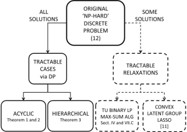
Fig. 1. Example of bipartite graph between variables and groups induced by the group structureG1, see Example 1 for details.
II. BASICDEFINITIONS
Let x ∈ RN be a vector, with dim(x) = N , and
N = {1, . . . ,N} be the set of its indices. We use |S| to denote the cardinality of an index set S. Given a vector x ∈ RN and a set S, we define xS ∈ R|S|, such that the components of xS are the components of x indexed by S. We use BN to represent the space of N -dimensional binary vectors and defineι:RN →BN to be the indicator function of the nonzero components of a vector inRN, i.e.,ι(x)i =1
if xi = 0 and ι(x)i = 0, otherwise. We let 1N to be the N -dimensional vector of all ones and IN the N×N identity
matrix. The support of x is defined by the set-valued function supp(x)= {i ∈N :xi =0}. Note that we normally use bold
lowercase letters to indicate vectors and bold uppercase letters to indicate matrices.
We start with the definition of total unimodularity, a prop-erty of matrices that will turn out to be key for obtaining efficient relaxations of integer linear programs.
Definition 1: A totally unimodular matrix (TU matrix) is
a matrix for which every square non-singular submatrix has determinant equal to−1 or 1.
We now define the main building block of group sparse model selection, the group structure.
Definition 2: A group structure G = {G1, . . . ,GM} is a collection of index sets, named groups, with Gj ⊆ N and
|Gj| =gj for 1≤ j ≤M and
G∈GG=N.
We can represent a group structureG as a bipartite graph, where on one side we have the N variables nodes and on the other the M group nodes. An edge connects a variable node i to a group node j if i ∈Gj. Fig. 1 shows an example. The
bi-adjacency matrix AG ∈ BN×M of the bipartite graph encodes the group structure,
AGi j =
1, if i ∈Gj;
0, otherwise.
Another useful representation of a group structure is via an
intersection graph (V,E) where the nodes V are the groups
G ∈ G and the edge set E contains ei j if Gi ∩Gj = ∅, that
is an edge connects two groups that overlap. A sequence of connected nodesv1, v2, . . . , vn, is a cycle ifv1=vn.
Example 1: In order to illustrate these concepts, consider
the group structure G1 defined by the following groups,
G1 = {1}, G2 = {2}, G3 = {1,2,3,4,5}, G4 = {4,6},
G5 = {3,5,7} and G6 = {6,7,8}. G1 can be represented by the variables-groups bipartite graph of Fig. 1 or by the
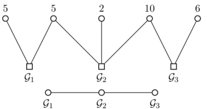
Fig. 2. Bipartite intersection graph with cycles induced by the group structureG1, where on each edge we report the elements of the intersection.
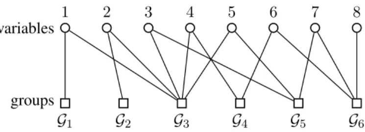
Fig. 3. (Left) Acyclic group structure. (Right) By adding one element fromG1intoG3, we introduce a cycle in the graph.
intersection graph of Fig. 2, which is bipartite and contains cycles.
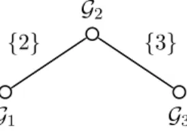
An important class of group structures is given by groups whose intersection graph is acyclic (i.e., a tree or a forest) and we call them acyclic group structures. A necessary, but not sufficient, condition for a group structure to have an acyclic intersection graph is that each element ofN occurs in at most two groups, i.e., the groups are at most pairwise overlapping. Note that a tree or a forest is a bipartite graph, where the two partitions contain the nodes that belong to alternate levels of the tree/forest. For example, consider G1 = {1,2,3}, G2 = {3,4,5}, G3 = {5,6,7}, which can be represented by the intersection graph in Fig. 3(Left). If G3 were to include an element from G1, for example{2}, we would have the cyclic graph of Fig. 3(Right). Note that G1is pairwise overlapping, but not acyclic, since G3,G4,G5 andG6form a cycle.
We anchor our analysis of the tractability of interpretability via selection of groups on covering arguments. Most of the definitions we introduce here can be reformulated as variants of set covers on the support of a signal x, however we believe it is more natural in this context to talk about group covers of a signal x directly.
Definition 3: A group cover S(x) for a signal x ∈ RN is a collection of groups such that supp(x) ⊆ G∈S(x)G. An alternative equivalent definition is given by
S(x)= {Gj ∈G:ω∈BM, ωj =1, AGω≥ι(x)}.
The binary vector ωindicates which groups are active and the constraint AGω ≥ ι(x) makes sure that, for every non-zero component of x, there is at least one active group that covers it. We also say thatS(x)covers x. Note that the group
cover is often not unique and S(x) = G is a group cover for any signal x. This observation leads us to consider more restrictive definitions of group covers.
Definition 4: A G-group cover SG(x) ⊆ G is a group cover for x with at most G elements,
SG( x)= {Gj ∈G: ω∈BM, ω j =1, AGω≥ι(x), M j=1 ωj ≤G}.
It is not guaranteed that a G-group cover always exists for any value of G. Finding the smallest G-group cover lead to the following definitions.
Definition 5: The group 0-“norm” is defined as xG,0:= min ω∈BM ⎧ ⎨ ⎩ M j=1 ωj :AGω≥ι(x) ⎫ ⎬ ⎭. (1)
A similar definition of group sparsity is also considered in [22]; however, there are also key differences in the concepts used for such definition. The authors use coding complexity as a lower bound on the “cost” required to cover a given subset ofN. Particularly, in the group sparsity case as defined in [22], each predefined group is assigned the coding complexity log2(2m), where m is the total number of groups in the model. Then, based on [22, Definition 2], the 0-“norm” for group sparsity is defined as the minimum coding length of the selected subset of groups: i.e., the summation of coding lengths for each group, such that the union of groups encoded “covers” the given support set. Thus, the resulting coding length in this case is g log2(2m), where g is the number of groups used in the covering. In our definition of group0-“norm”, we assign a unitary cost to each selected group, such that each non-zero element in x is covered by at least one active group.
Definition 6: A minimal group cover for a signal x∈RN
is defined asM(x)≡ {Gj ∈ G : ˆω(x)j =1}, where ωˆ is a minimizer for (1), ˆ ω(x)∈argmin ω∈BM ⎧ ⎨ ⎩ M j=1 ωj :AGω≥ι(x) ⎫ ⎬ ⎭.
A minimal group cover M(x) is a group cover for the support of x with minimal cardinality. Note that there exist pathological cases where for the same group 0-“norm”, we have different minimal group cover models. The minimal group cover can also be seen as the minimum set cover of the support of x.
Definition 7: A signal x is G-group sparse with respect
to a group structureGif xG,0≤G.
In other words, a signal is G-group sparse if its support is contained in the union of at most G groups fromG.
III. TRACTABILITY OFINTERPRETATIONS
Although real signals may not be exactly group-sparse, it is possible to give a group-based interpretation by finding a group-sparse approximation and identifying the groups that constitute its support. In this section, we establish the hardness of group-constrained approximations of signals in general and characterize a class of group structures that lead to tractable approximations. In particular, we present a polynomial time algorithm that finds the correct G-group-support of the
G-group-sparse approximation of x, given a positive integer G and the group structureG.
We first define the G-group sparse approximation x andˆ then show that it can be easily obtained from its G-group cover SG(xˆ), which is the solution of the model selection problem. We then reformulate the model selection problem as the weighted maximum coverage problem. Finally, we present
our main result, the polynomial time dynamic program for acyclic group structures.
Signal Approximation Problem: Given a signal x ∈ RN, a best G-group sparse approximationx is given byˆ
ˆ x∈argmin z∈RN x−z2 2: zG,0≤G . (2)
If we already know the G-group cover of the approximation
SG(xˆ), we can obtain x asˆ xˆ
I = xI and xˆIc = 0, where I =G∈SG(xˆ)GandIc=N\I. Therefore, we can solve (2) by solving the following discrete problem.
Model Selection Problem: Given a signal x ∈ RN, a G-group cover model for its G-group sparse approximation is expressed as follows SG(ˆ x)∈argmax S⊆G ⎧ ⎨ ⎩ i∈I xi2:I= G∈S G, |S| ≤G ⎫ ⎬ ⎭. (3)
To show the connection between the two problems, we first reformulate (2) as min z∈RN x−z 2 2 subject to supp(z)=I, I= G∈S G S ⊆G, |S| ≤G, (4)
which can be rewritten as min S⊆G |S| ≤G I=G∈SG min z∈RN supp(z)=I x−z22.
The optimal solution is not changed if we introduce a constant, change sign of the objective and consider maximization instead of minimization max S⊆G |S| ≤G I=G∈SG max z∈RN supp(z)=I x2 2− x−z22 .
The internal maximization is achieved for x asˆ xˆI =xI and ˆ
xIc=0, so that we have, as desired, SG(xˆ)∈ argmax
S⊆G |S| ≤G
I=G∈SG xI22.
The following reformulation of (3) as a binary problem allows us to characterize its tractability.
Lemma 1: Given x ∈ RN and a group structure G, we have thatSG(xˆ)= {Gj ∈G:ωGj =1}, where(ωG,yG)is an optimal solution of max ω∈BM,y∈BN ⎧ ⎨ ⎩ N i=1 yixi2:AGω≥y, M j=1 ωj ≤G ⎫ ⎬ ⎭. (5)
Proof: The proof follows along the same lines as the proof in [29]. Note that in (5), ω and y are binary variables that specify which groups and which variables are selected, respectively. The constraint AGω ≥ y makes sure that for every selected variable at least one group is selected to cover it, while the constraint Mj=1ωj ≤G restricts choosing at most
G groups.
Problem (5) can produce all the instances of the weighted maximum coverage problem (WMC), where the weights for each element are given by x2
i (1≤i ≤N ) and the index sets
are given by the groups Gj ∈G (1≤ j ≤ M). Since WMC
is NP-hard [27] and given Lemma 1, the tractability of (3) directly depends on the hardness of (5), which leads to the following result.
Proposition 1: The model selection problem (3) is
NP-hard.
It is possible to approximate the solution of (5) using the greedy WMC algorithm [32]. At each iteration, the algorithm selects the group that covers new variables with maximum combined weight until G groups have been selected. However, we show next that for certain group structures we can find an exact solution.
Our main result is an algorithm for solving (5) for acyclic group structures.
Theorem 1: Given an acyclic group structure G with M groups and a group budget G, the dynamic programming algorithm described in Section VIII-B solves (5) in O(G M2) time.
The proof of a more general algorithm, which also includes a sparsity budget, is given in Appendix A, while an intuitive description of the algorithm is given in Section VIII-B.
Remark 1: It is also possible to consider the case where
each group Gi has a cost Ci and we are given a maxi-mum group cost budget C. The problem then becomes the Budgeted Maximum Coverage [33]. However, this problem is NP-hard, even in the non-overlapping case, because it generalizes the knapsack problem. However, similarly to the pseudo-polynomial time algorithm for knapsack [34], we can easily devise a pseudo-polynomial time algorithm for the weighted group sparse problem, even for acyclic overlaps. The only condition is that the costs must be integers. The time complexity of the resulting algorithm is then polynomial in C, the maximum group cost budget. The algorithm is almost the same as the one given in Appendix A: instead of keeping track of selecting g groups, where g varies from 1 to G; we keep track of selecting groups with total weight equal to c, where c varies from 1 to C.
IV. DISCRETERELAXATIONS
Relaxations are useful techniques that allow to obtain approximate, or sometimes even exact solutions. In the spe-cific cases below, relaxations provide less computationally demanding solutions. In our case, we relax the constraint on the number of groups in (5) into a regularization term with parameter λ > 0, which amounts to paying a penalty of λ for each selected group. We then obtain the following binary linear program (ωλ,yλ)∈ argmax ω∈BM, y∈BN AGω≥y ⎧ ⎨ ⎩ N i=1 yixi2−λ M j=1 ωj ⎫ ⎬ ⎭ (6)
We can rewrite the previous program in standard form. Let u = [y ω] ∈ BN+M, w = [x12, . . . ,x2N,−λ1M] ∈
RN+M and C= [I
that (6) is equivalent to uλ∈argmax u∈BN+M wu:Cu≤0 (7) In general, (7) is NP-hard, however, it is well known [28] that if the constraint matrix C is Totally Unimodular (TU), then it can be solved in polynomial-time. While the concatenation of two arbitrary TU matrices is not TU, the concatenation of the identity matrix with a TU matrix results in a TU matrix. Thus, due to its structure, C is TU if and only if AG is TU [28, Proposition 2.1].
The next lemma characterizes which group structures lead to totally unimodular constraints.
Proposition 2: Group structures whose intersection graph
is bipartite lead to constraint matrices AGthat are TU. Proof: We first use a result that establishes that if a matrix
is TU, then its transpose is also TU [28, Proposition 2.1]. We then apply [28, Corollary 2.8] to AG, swapping the roles of rows and columns. Given a {0,1,−1}matrix whose columns can be partitioned into two sets,S1andS2, and with no more than two nonzero elements in each row, this corollary provides two sufficient conditions for it being totally unimodular:
1) If two nonzero entries in a row have the same sign, then the column of one is inS1 and the other is inS2. 2) If two nonzero entries in a row have opposite signs, then
their columns are both in S1 or both inS2.
In our case, the columns of AG, which represent groups, can be partitioned in two sets,S1 andS2 because the intersection graph is bipartite. The two sets represents groups which have no common overlap so that each row of AGcontains at most two nonzero entries, one in each set. Furthermore, the entries in AG are only 0 or 1, so that condition 1) is satisfied and
condition 2) does not apply.
Corollary 1: Acyclic group structures lead to totally
uni-modular constraints.
Proof: Acyclic group structures have an intersection graph
which is a tree or a forest, which is bipartite.
The worst case complexity for solving the linear pro-gram (7), via a primal-dual method [35], isO(N2(N+M)1.5), which is greater than the complexity of the dynamic program of Theorem 1. However, in practice, using an off-the-shelf LP solver may still be faster, because the empirical performance is usually much better than the worst case complexity.
Another way of solving the linear program for acyclic group structures is to reformulate it as an energy maximization problem over a tree, or forest. In particular, let ψi = xGi
2 2 be the energy captured by groupGi andψi j = xGi∩Gj
2 2 the energy that is double counted if bothGi andGj are selected,
which then needs to be subtracted from the total energy. Consider first problem (3). Given the energy functions defined above, the objective in the maximization can be rewritten as:
i∈I xi2= xI22 = M i=1 ωixGi 2 2− (i,j)∈E ωiωjxGi∩Gj 2 2 = M i=1 ωiψi− (i,j)∈E ωiωjψi j. (8)
Here, the first term corresponds to the energy contributed by the active groups and the second term corresponds to the excessive energy contributed by the overlapping active groups, and thus needs to be removed. The regularized version, problem (6), can then be formulated as
max ω∈BM M i=1 ωi(ψi −λ)− (i,j)∈E ωiωjψi j.
This problem is equivalent to finding the most probable state of the binary variables ωi, where their probabilities can be
factored into node and edge potentials. These potentials can be computed inO(N)time via a single sweep over the elements, then the most probable state can be exactly estimated by the max-sum algorithm in onlyO(M)operations, by sending messages from the leaves to the root and then propagating other message from the root back to the leaves [31].
The next lemma establishes when the regularized solution coincides with the solution of (5).
Lemma 2: If the value of the regularization parameterλ
is such that the solution(ωλ,yλ)of (6) satisfiesjωλj =G, then(ωλ,yλ)is also a solution for (5).
Proof: This lemma is a direct consequence of
Proposition 3 below.
However, as we numerically show in Section IX, given a value of G it is not always possible to find a value ofλsuch that the solution of (6) is also a solution for (5). Let the set of pointsP = {G, (f(G))}GM=1, where f(G)=iN=1yiGxi2, be
the Pareto frontier of (5) between approximation quality and group budget. We then have the following characterization of the solutions of the discrete relaxation.
Proposition 3: The discrete relaxation (6) yields only the
solutions that lie on the intersection between the Pareto frontier P of (5), as defined above, and the boundary of the convex hull ofP.
Proof: The solutions of (5) for all possible values of G
are the Pareto optimal solutions [36, Sec. 4.7] of the follow-ing vector-valued minimization problem with respect to the positive orthant ofR2, which we denote by R2+,
min ω∈BM,y∈BN f(ω,y) subject to AGω≥y (9) where f(ω,y) = x2−N i=1yixi2, M j=1ωj ∈ R2 +.
Specifically, the two components of the vector-valued func-tion f are the approximafunc-tion error E, and the number of groups G that cover the approximation. It is not possible to simultaneously minimize both components, because they are somehow adversarial: unless there is a group in the group structure that covers the entire support of x, lowering the approximation error requires selecting more groups. Therefore, there exists the so called Pareto frontier of the vector-valued optimization problem defined by the points(EG,G)for each
choice of G, i.e., the second component of f, where EG is
the minimum approximation error achievable with a support covered by at most G groups.
The scalarization of (9) yields the following discrete prob-lem, with λ >0 min ω∈BM,y∈BN x 2− N i=1 yixi2+λ M j=1 ωj subject to AGω≥y (10)
whose solutions are the same as for (6). Therefore, the rela-tionship between the solutions of (5) and (6) can be inferred by the relationship between the solutions of (9) and (10). It is known that the solutions of (10) are also Pareto optimal solutions of (9), but only the Pareto optimal solutions of (9) that admit a supporting hyperplane for the feasible objective values of (9) are also solutions of (10) [36, Sec. 4.7]. In other words, the solutions obtainable via scalarization belong to the intersection of the Pareto optimal solution set and the boundary
of its convex hull.
V. CONVEXRELAXATIONS
For tractability and analysis, convex proxies to the group 0-norm have been proposed (e.g., [23]) for finding group-sparse approximations of signals. Given a group structure G, an example generalization is defined as
xG,{1,p}:= inf v1, . . . ,vM∈RN ∀j,supp(vj)=Gj M j=1vj=x M j=1 djvjp (11) where xp = iN=1x p i 1/p
is the p-norm, and dj are
positive weights that can be designed to favor certain groups over others [11]. This norm, also called Latent Group Lasso norm in the literature, can be seen as a weighted instance of the atomic norm described in [8], where the authors leverage convex optimization for signal recovery, but not for model selection.
One can use (11) to find a group-sparse approximation under the chosen group norm
ˆ x∈argmin z∈RN x−z2 2: zG,{1,p}≤λ , (12)
where λ > 0 controls the trade-off between approximation accuracy and group-sparsity. However, solving (12) does not yield a group-support for x: though we can recover oneˆ through the decomposition {vj} used to computeˆxG,{1,p},
it may not be unique as observed in [11] for p = 2. In order to characterize the group-support for x induced by (11), in [11] the authors define two group-supports for p = 2. The strong group-support S˘(x) contains the groups that constitute the supports of each decomposition used for computing (11). The weak group-support S(x) is defined using a dual-characterisation of the group norm (11). If S˘(x) = S(x), the group-support is uniquely defined. However, [11] observed that for some group structures and signals, even whenS˘(x)=S(x), the group-support does not capture the minimal group-cover of x.
Hence, the equivalence of 0 “norm” and 1 norm mini-mization [2], [3] in the standard compressive sensing setting
Fig. 4. The intersection graph for the example in Section VI.
does not hold in the group-based sparsity setting. Therefore, even for acyclic group structures, for which we can obtain exact identification of the group support of the approximations via dynamic programming, the convex relaxations are not guaranteed to find the correct group support. We illustrate this case via a simple example in the next section. It remains an open problem to characterize which classes of group structures and signals admit an exact identification via convex relaxations.
VI. CASESTUDY: DISCRETE VS. CONVEXINTERPRETABILITY
The following stylized example illustrates situations that can potentially be encountered in practice. In these cases, the group-support obtained by the convex relaxation will not coincide with the discrete definition of group-cover, while the dynamical programming algorithm of Theorem 1 is able to recover the correct group-cover.
Let N = {1, . . . ,4} and let G = {G1 = {1,2}, G2 = {2,3}, G3 = {3,4}} be an acyclic group structure structure with three groups of equal cardinality. Its intersection graph is represented in Fig. 4. Consider the 2-group sparse signal x= [1 2 2 1], with minimal group-coverM(x)= {G1,G3}. The dynamic program of Theorem 1, with group budget
G = 2, correctly identifies the groups G1 and G3. The TU linear program (6), with 0 < λ ≤ 2, also yields the correct group-cover. By contrast, the decomposition obtained via (11) with unitary weights and p = 2 is unique, but is not group sparse. In fact, we have S(x) = ˘S(x) = G. We can only obtain the correct group-cover if we use the weights [1 d 1] with d>
8
5, that is knowing beforehand thatG2is irrelevant. These results are obtained directly from (11), exploiting the symmetry in both the group structure and x to simplify the problem to one variable depending on d.
Remark 2: This is an example where the correct minimal
group-cover exists, but cannot be directly found by the Latent Group Lasso approach. There may also be cases where the minimal group-cover is not unique. We leave to future work, to investigate which of these minimal covers are obtained by the proposed dynamic program and characterize the behavior of relaxations.
VII. GENERALIZATIONS
In this section, we first present a generalization of the discrete approximation problem (5) by introducing an addi-tional overall sparsity constraint. Secondly, we show how this generalization encompasses approximation with hierarchical constraints that can be solved exactly via dynamic program-ming. Finally, we show that the generalized problem can be
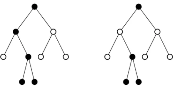
Fig. 5. Hierarchical constraints. Each node represent a variable, in black selected variables. (Left) A valid selection of nodes. (Right) An invalid selection of nodes.
relaxed into a linear binary problem and that hierarchical constraints lead to totally unimodular matrices for which there exist efficient polynomial time solvers.
A. Sparsity Within Groups
In many applications, for example genome-wide association studies [17], it is desirable to find approximations that are not only group-sparse, but also sparse in the usual sense (see [37] for an extension of the group lasso). To this end, we generalize our original problem (5) by introducing a sparsity constraint K and allowing to individually select variables within a group; then, one could use such projection step in linear regression frameworks, in order to impose such structure in the final solution. The generalized integer problem then becomes max ω∈BM,y∈BN N i=1yix 2 i subject to AGω≥y N i=1yi ≤K M j=1ωj ≤G. (13) The problem described above is a generalization of the well-known Weighted Maximum Coverage (WMC) problem. The latter does not have a constraint on the number of indices chosen, so we can simulate it by setting K =N . WMC is also
well-known to be NP-hard, so that our present problem is also NP-hard, but it turns out that it can be solved in polynomial time for the same group structures that allow to solve (5).
Theorem 2: Given an acyclic group structure G with
M groups, a group budget G and a sparsity budget K , Algorithm 1 solves (13) in O(M2G K2)time.
An intuitive description of the algorithm is given in Section VIII-A, together with its pseudocode. The dynamic program is thoroughly described in Appendix A, which also contains the proof of its time complexity.
B. Hierarchical Constraints
The generalized model allows to deal with hierarchical structures, such as regular trees, frequently encountered in image processing (e.g., denoising using wavelet trees). In such cases, we often require to find K -sparse approximations such that the selected variables form a rooted connected subtree of the original tree, see Fig. 5. Given a tree T, the rooted-connected approximation can be cast as the solution of the
Algorithm 1 Tree-WMC With Sparsity (TWMCS)
Inputs: Acyclic group structure G consisting of M groups defined over N elements, weights of N elements, group budget G, sparsity budget K .
Output: Set of K elements contained in G groups with maximum combined weight.
1: Initialize rooted tree T with vertex set G correspond-ing to the M groups, edge set E corresponding to edges between overlapping groups, and root chosen arbitrarily.
2: Compute the Graph Exploration Rule using Algorithm 5 (Appendix A-G).
3: Recursively compute the table of optimal values via the Value Update Rule using Algorithm 3 (Appendix A-F). 4: Backtrack the optimal selection of G groups and K
ele-ments from Algorithm 4 (Appendix A-F).
Algorithm 2 Rooted Connected K -Sparse Trees
Input: Rooted tree T(V,E,root) of N nodes, weights of nodes, sparsity budget K .
Output: A subtree ofT with the same root asT, having at most K nodes with maximum combined weight.
1: Recursively compute the table of optimal values with the Value Update Rule using Algorithm 6 (Appendix B-C). 2: Backtrack the optimal selection of at most K nodes using
Algorithm 7 (Appendix B-E).
following discrete problem max y∈BN N i=1 yixi2:supp(y)∈TK , (14)
where TK denotes all rooted and connected subtrees of the
given treeT with at most K nodes.
This type of constraints can be represented by a group structure, where for each node in the tree we define a group consisting of that node and all its ancestors. When a group is selected, we require that all its elements are selected as well. We impose an overall sparsity constraint K , while discarding the group constraint G.
Relaxed and greedy approximations have been pro-posed [38]–[40] for this particular problem. In Section VIII-C, we describe a dynamic program, Algorithm 2, that runs in polynomial time and yields an exact solution, while Appendix B contains a formal description and proofs of its correctness and time-space complexity.
Theorem 3: Given a tree with N nodes and maximum
degree D, Algorithm 2 solves (14) in O(N K2D)time. While preparing the final version of this manuscript, [41] independently proposed a similar dynamic program for tree projections on D-regular trees with time complexity
O(N K D). Following their approach, we improved the time complexity of our algorithm toO(N K D)for D-regular trees. We also prove that its memory complexity is O(N logDK).
A computational comparison of the two methods, both imple-mented in Matlab, is provided in Section IX, showing that our
dynamic program can be up to 60 times faster, despite having similar worst-case time complexity.
Proposition 4: The time complexity of Algorithm 2 on
D-regular trees isO(N K D).
Proposition 5: The space complexity of Algorithm 2 on
D-regular trees isO(N logDK).
The proofs of both propositions can be found in Appendix B.
C. Additional Relaxations
By relaxing both the group budget and the sparsity budget in (13) into regularization terms, we obtain the following binary linear program
(ωλ,yλ)∈ argmax ω∈BM,y∈BN wu subject to u= [y ω y] Cu≤0 (15) where w = [x2 1, . . . ,x2N,−λG1M,−λK1N] and C =
[IN,−AG, 0N] and λG, λK > 0 are two regularization
parameters that indirectly control the number of active groups and the number of selected elements. (15) is of the same form as (7), therefore can be solved in polynomial time if the constraint matrix C is totally unimodular. Due to its structure, by [28, Proposition 2.1] and that concatenating a matrix of zeros to a TU matrix preserves total unimodularity, C is totally unimodular if and only if AG is totally unimodular. As a characteristic example of when such cases appear in practice, we provide the following proposition.
Proposition 6: Hierarchical group structures lead to totally unimodular constraints.
Proof: We use the fact that a binary matrix is totally unimodular if there exists a permutation of its columns such that in each row the 1s appear consecutively, which is a combination of [28, Corollary 2.10 and Proposition 2.1]. For hierarchical group structures, such permutation is given by a depth-first ordering of the groups. In fact, a variable is included in the group that has it as the leaf and in all the groups that contain its descendants. Given a depth-first ordering of the groups, the groups that contain the descendants of a given
node will be consecutive.
The regularized hierarchical approximation problem, in par-ticular max y∈BN N i=1 yixi2−λy0: supp(y)∈TN , (16)
forλ≥0, has already been addressed by Donoho et al. [42] as the dyadic CART, which can find a solution inO(N)time. However, it is not clear how to set the regularization parame-ter λ in order to obtain solutions with a given sparsity bud-get K . The condensing sort and select algorithm (CSSA) [38], with complexityO(N log N), solves problem (16) where the indicator variable y is relaxed to be continuous in [0,1]and the penalty term is substituted with the constraint that y1 be smaller than a given threshold γ, yielding rooted con-nected approximations that might have more than K elements.
Moreover, applying the heuristic to threshold the final solution to obtain a K -sparse solution does not guarantee to return the best K -sparse tree projection.
VIII. ALGORITHMS
In this section, we provide an outline of our two dynamic programming algorithms for solving problems (13) and (14), respectively. Additional algorithmic considerations can be found in the appendices.
A. Tree-WMC With Sparsity
One of the key contributions of this work is a new dynamic programming algorithm which solves problem (13). Our algorithm addresses the following question: Given N items contained in M groups, and each item associated with a non-negative weight, how can we choose G groups, and
K items within these G groups, in order to maximize the
sum of weights of the chosen items? This problem is NP-hard since it generalizes the Weighted Maximum Coverage (WMC) problem. However, if the intersection graph is a tree (or a forest), then the problem can be solved in polynomial time, as we briefly describe next and prove in Appendix A. We note that our dynamic programming algorithm can be easily generalized to the case where groups and items have integral costs instead of unit costs, giving us a pseudo-polynomial time scheme.
Broadly speaking, the proposed framework is a dynamic program, i.e., it builds the solution to the global problem from solutions of sub-problems. In our case, the sub-problem involves a subset of the groups. To introduce the key steps of our approach gradually, let us first consider the following idea: Looking at a subsetSn of groups, one might compute a
table of optimal g-group sparse, k-element sparse solutions
for all 1 ≤ g ≤ G,1 ≤ k ≤ K . Then, we might try
to extend this table by adding one new group Gn+1 to Sn,
as in standard dynamic programming approaches. Unfortu-nately, such an approach fails to find the optimal solution. To see this, observe that in order to perform such an extension, it is essential to know whether the new items appearing in
Gn+1have already been considered forSn; otherwise, it could
lead to double-counting, which happens when Gn+1overlaps with some groups inSn.1
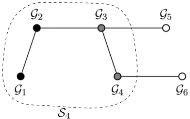
To rectify this, we introduce the notion of a boundary group,
i.e., a group within the current selected subset of groups, that
may overlap with future groups. Thus, the boundary groups of
Sn are all the groups inSn which overlap with some group in
G\Sn; see also Figure 6. Our idea is to store a separate
table of solutions for each possible selection of boundary groups, i.e., all 2b combinations for b boundary groups. The fact that we can avoid double-counting in this manner is non-obvious: It relies on an optimal substructure property that we describe in Appendix A-B. Leveraging this property, we show the existence of a value update rule (Appendix A-F), which allows us to extend our solutions by incorporating one new
1While such argument provides intuition, it does not rigorously prove that the above method could not succeed; we refer the reader to appendix A for a detailed analysis.
Fig. 6. Boundary groups: In the intersection graph above, the set of explored groups isS4= {G1,G2,G3,G4}. The boundary groups are{G3,G4}.
group at a time. Repeating this rule, we eventually obtain the global optimal solution.
Remark 3: Sets that are included in one another can be
excluded because choosing the larger set would be a strictly dominant strategy, making the smaller set redundant. However, the correctness of the dynamic program is unaffected even if such sets are present, as long as the intersection graph remains acyclic.
The above procedure adds a factor of 2bto our running time,
which can be exponential.2 In Appendix A-G, we show that we can design a graph exploration rule for tree intersection graphs, which prevents the number of boundary groups from growing too large. In fact, the maximum number of boundary groups, when an acyclic intersection graph is explored using our method, is bounded by log2M for M groups. This further implies that the factor 2b remains bounded by M throughout our algorithm, which leads to a polynomial running time of
O(M2K2G).
The Tree-WMC with Sparsity (TWMCS) pseudocode is provided in Algorithm 1, while Appendices A-G and A-F describe the graph exploration rule and the value update rule in Algorithms 5 and 3, respectively. Once the final table of optimal values has been computed, it is necessary to backtrack the algorithm’s steps in order to obtain the optimal solution. This backtracking procedure is outlined in Algorithm 4 in Appendix A-F.
B. Tree-WMC Without Sparsity
If there is no sparsity budget K , the dynamic program described in the previous section can be simplified to effi-ciently solve (5) for acyclic group structures. The first key observation is that it is sufficient to keep a smaller table of optimal values without considering the sparsity variable. Secondly, in the value update step, when the new group is selected, we add all its elements after removing any overlap with the boundary groups.
Here, we encounter a potential problem—if there exist groups with a large number of elements, the value update step could add a factor of O(N) to the complexity. This problem
2Indeed, if the factor was always polynomial, we could solve an NP-hard problem.
can be easily avoided with some pre-processing, where we combine elements into equivalent groups based on the overlap structure. Since sparsity is no longer a constraint, if two elements are contained in the same set of groups, they can be treated as one element with the combined weight. Due to the tree structure, this will result in at most O(M)different elements3once the pre-processing is complete i.e., same order of elements as number of groups. It can be shown that after this operation, adding element weights will not increase the complexity. The final time complexity of Algorithm 1 in this case isO(G M2).
C. Rooted, Connected K -Sparse Trees
We describe here the Dynamic Programming algorithm that solves problem (14). In this case, we are interested in the following question: Given a rooted tree with a non-negative weight associated with each node, how can we pick K nodes that form a rooted, connected subtree in order to maximize the sum of weights of the nodes? By rooted, connected subtree, we mean that the root must be selected, and for any selected node, all of its ancestors up to the root must also be chosen.
An interesting feature of the rooted-connected subtree con-straint is the following: Let T0 be the maximum-weight, K -node, rooted, connected subtree in our graph. For any
node X , consider the subset of nodes in T0which are descen-dants of X . Then, these form a rooted, connected subtree at
X (call it TX). Further, if TX comprises k nodes, then TX is
the maximum-weight, k-node, rooted, connected subtree at X . This suggests a natural choice of sub-problems for dynamic programming.
Briefly, our objective is to compute the optimal weights of all k-node, rooted, connected subtrees at any node X , for each
k∈ {1, . . . ,K}. If X is a leaf node, this is trivial. If X is not a
leaf node, then we shall inductively assume that these solutions have been computed for all of its subtrees. To combine the subtrees at X , we use the following Value Update Rule: The optimal way to choose k nodes from two subtrees equals the optimal way to choose k − j nodes from the first subtree
and j nodes from the second subtree, maximized over all
j∈ {0, . . . ,k}. A detailed analysis of this algorithm leads to a running time ofO(N K D)for D-regular trees, andO(N K2D)
for trees which have maximum degree D, but may not be
D-regular (see Appendix B-D). Algorithm 2 summarizes the
key steps of the dynamic program, whose details and analysis are given in Appendix B.
IX. PARETOFRONTIEREXAMPLES
The purpose of these numerical simulations is to illustrate the limitations of relaxations and of greedy approaches for correctly estimating the G-group cover of an approximation.
A. Acyclic Constraints
We consider the problem of finding a G-group sparse approximation of the wavelet coefficients of a given image,
3After pre-processing, there will be at most one element corresponding to each node and each edge of the tree intersection graph.
Fig. 7. Insets: (Left) Earth image used for the numerical simulation, before being resized to 16×16 pixels. (Right) Example of allowed support on one of the three wavelet quad-trees: The black circles represent selected variables and the empty circles unselected ones, while the dotted triangles indicate the active groups. Main plot: 2D Wavelet approximation on three quad-trees. The original signal is the wavelet decomposition of the 16×16 pixels Earth image. The blue line is the Pareto frontier of the dynamic program for all group budgets G. Note that, for G≥52, the approximation error for the dynamic program is zero, while the Latent Group Lasso approach needs to select all 64 groups to yield a zero error approximation. The totally unimodular relaxation only yields the points in the Pareto frontier of the dynamic program that lie on its convex hull.
in our case a view of the Earth from space, see left inset in Fig. 7. We consider a group structure defined over the 2D wavelet tree. The wavelet coefficients of a 2D image can naturally be organized on three regular quad-trees, cor-responding to a multi-scale analysis with wavelets oriented vertically, horizontally and diagonally, respectively [1]. We define groups consisting of a node and its four children, therefore each group has 5 elements, apart from the topmost group that contains the scaled average term and the first nodes of each of the three quad-trees. These groups overlap only pairwisely and their intersection graph is a tree itself, therefore leading to a totally unimodular constraint matrix. An example is given in the right inset in Fig. 8. We resize the image to 16×16 pixels and compute its Daubechies-4 wavelet coeffi-cients. At this size, there are 64 groups, but actually 52 are sufficient to cover all the variables, since it is possible to ignore the penultimate layer of groups.
Figures 7 and 8 show the Pareto frontier of the approxi-mation error x− ˆx22 with respect to the group sparsity G for the proposed dynamic program, Algorithm 1. We also report the approximation error for the solutions obtained via the totally unimodular linear relaxation (TU-relax) (7) and the latent group lasso formulation (Latent GL) (12) with p = 2, which we solved with the method proposed in [43]. Fig. 8 shows the performance of StructOMP [22] using the same group structure and of the greedy algorithm
for solving the corresponding weighted maximum coverage problem.
We observe that there are points in the Pareto frontier of the dynamic program, for G = 5,10,30,31,50, that are not achievable by the TU relaxation, since they do not belong to its convex hull. Furthermore, the latent group lasso approach often does not yield the optimal selection of groups, leading to a greater approximation error for the same number of active groups and it needs to select all 64 groups in order to achieve zero approximation error. It is interesting to notice that the greedy algorithm outperforms StructOMP (see inset of Fig. 8), but still does not achieve the optimal solutions of the dynamic program. Furthermore, StructOMP needs to select all 64 groups for obtaining zero approximation error, while the greedy algorithm can do with one less, namely 63.
B. Hierarchical Constraints
We now consider the problem of finding a K -sparse approx-imation of a signal imposing hierarchical constraints. We gen-erate a piecewise constant signal of length N =64, to which we apply the Haar wavelet transformation, yielding a 25-sparse vector of coefficients x that satisfies hierarchical constraints on a binary tree of depth 5, see Fig. 9(Top).
We compare the proposed dynamic program (DP),
Fig. 8. 2D Wavelet approximation on three quad-trees. The original signal is the wavelet decomposition of the 16×16 pixels Earth image. The blue line is the Pareto frontier of the dynamic program for all group budgets G. Note that for G≥52 the approximation error for the dynamic program is zero, while StructOmp needs to select all 64 groups to yield a zero error approximation. The greedy algorithm for solving the corresponding weighted maximum coverage problem obtains better solutions than StructOmp, but it still requires 63 groups to yield a zero-error approximation.
Fig. 9. (Top) Original piecewise constant signal and its Haar wavelet representation. (Bottom) Signal approximation on the binary tree. The original signal is 25-sparse and satisfies hierarchical constraints. The numbers next to the Parent-Child solutions indicate the number of hierarchial constraint violations, i.e., a node is selected but not its parent.
program approach, two convex relaxations that use group-based norms and the StructOMP greedy approach [22]. The first convex relaxation [8] uses the Latent Group Lasso
norm (11) with p =2 as a penalty and with groups defined as all parent-child pairs in the tree. We call this approach Parent-Child. This formulation will not enforce all hierarchical
Fig. 10. Running times in seconds of the proposed dynamic program for hierarchical constraints and the one proposed by Cartis and Thompson [41]. The sparsity budget is kept constant to K=200 for all problem sizes.
constraints to be satisfied, but will only favor them. Therefore, we also report the number of hierarchical constraint violations. The second convex relaxation [40] considers a hierarchy of groups whereGj contains node j and all its descendants.
Hier-archical constraints are enforced by the group lasso penalty G L(x) = G∈GxGp, where xG is the restriction of x
to G, and we assess p = 2 and p = ∞. We call this
method Hierarchical Group Lasso. As shown in [30], solving minxy−x22+λG L(x), for p= ∞, is actually equivalent
to solving the totally unimodular relaxation with the same regularization parameter. Once we determine the support of the solution, we assign to the components in the support the values of the corresponding components of the original signal. Finally, for the StructOMP4 method, we define a block for each node in the tree. The block contains that node and all its ancestors up to the root. By finely varying the regularization parameters for these methods, we obtain solutions with different levels of sparsity.
In Figures 9(Bottom), we show the approximation error x − ˆx2
2 as a function of the solution sparsity K for the methods. The values of the DP solutions form the discrete Pareto frontier of the optimization problem controlled by the parameter K , indicated as Tree model in the figure. Note that there are points in the Pareto frontier that do not lie on its convex hull, hence these solutions are not achievable by the TU linear relaxation. As expected, the Hierarchical Group Lasso5 with p = ∞ obtains the same solutions as the TU linear relaxation, while with p=2 it also misses the solutions
for K = 21 and K = 23. The Parent-Child6 approach
achieves more levels of sparsity, but still misses the solutions for K =2,13 and 15. However, it also violates some of the hierarchical constraints, i.e., we count one violation when one node is selected but not its parent. The StructOMP approach yields only few of the solutions on the Pareto frontier, but without violating any constraints. These observations lead us to conclude that, in some cases, relaxations of the original
4We used the code provided at http://ranger.uta.edu/~huang/ R_StructuredSparsity.htm
5We used the code provided at http://spams-devel.gforge.inria.fr/. 6We used the algorithm proposed in [43].
discrete problem or other greedy approaches might not be able to find the correct group-based interpretation of a signal.
In Fig. 10, we report a computational comparison between our dynamic program, Algorithm 2, and the one independently proposed by Cartis and Thompson [41]. We consider the problem of finding the K = 200 sparse rooted connected tree approximation on a binary tree of a signal of length 2L, with L = 9, . . . ,18, whose components are randomly and uniformly drawn from[0,1]. Despite the two algorithms have the same computational complexity,O(N K D), and are both implemented in Matlab, our dynamic program is from 20 to 60 times faster.
X. CONCLUSIONS
Several applications benefit from group sparse represen-tations. Unfortunately, our main result shows that finding a group-based interpretation of a signal is an NP-hard integer optimization problem. To this end, we characterize group structures for which a dynamical programming algorithm can find a solution in polynomial time and also delineate discrete relaxations for special structures (i.e., totally unimodular con-straints) that can obtain correct solutions.
Our examples and numerical simulations show the defi-ciencies of relaxations, both convex and discrete, and of greedy approaches. We observe that relaxations only recover group-covers that lie in the convex hull of the Pareto frontier determined by the solutions of the original integer problem for different values of the group budget G (and sparsity budget K for the generalized model). This, in turn, implies that convex and non-convex relaxations might miss some important groups or include spurious ones in the group-sparse model selection. We summarize our findings in Fig. 11.
There remain several interesting open questions which deserves further studies. Firstly, an intuitive understanding of under which circumstances the relaxations are able to yield the correct solutions is still missing. Secondly, our analysis implicitly assumes an orthogonal basis for the description of signals. In many machine learning and compressive sens-ing applications however, the structures in signals emerge only after representing them onto an overcomplete basis,
![Fig. 10. Running times in seconds of the proposed dynamic program for hierarchical constraints and the one proposed by Cartis and Thompson [41]](https://thumb-us.123doks.com/thumbv2/123dok_us/11109184.2998695/13.918.165.752.87.326/running-seconds-proposed-dynamic-hierarchical-constraints-proposed-thompson.webp)