Robust Bayesian Seemingly Unrelated Regression Model
1Chamberlain Mbaha, Kris Peremansb, Stefan Van Aelstb and Dries F. Benoitc
a
Department of Basic Medical Sciences, Ghent University, Proeftuinstraat 86, B-9000 Ghent, Belgium
bDepartment of Mathematics, Section of Statistics, KU Leuven, Celestijnenlaan 200B, B-3001 Leuven, Belgium c
Faculty of Economics and Business Administration, Ghent University, Tweekerkenstraat 2, B-9000 Ghent, Belgium
August 24, 2018
Abstract: A robust Bayesian model for seemingly unrelated regression is proposed. By using heavy-tailed distributions for the likelihood, robustness in the response variable is attained. In addition, this robust procedure is combined with a diagnostic approach to identify observations that are far from the bulk of the data in the multivariate space spanned by all variables. The most distant observations are downweighted to reduce the effect of leverage points. The resulting robust Bayesian model can be interpreted as a heteroscedastic seemingly unrelated regression model. Robust Bayesian estimates are obtained by a Markov Chain Monte Carlo approach. Complications by using a heavy-tailed error distribution are resolved efficiently by representing these distributions as a scale mixture of normal distributions. Monte Carlo simulation experiments confirm that the proposed model outperforms its traditional Bayesian counterpart when the data are contaminated in the response and/or the input variables. The method is demonstrated on a real dataset.
Keywords: Conjugate Prior, Diagnostic Procedure, Heavy-tailed Distributions, Markov Chain Monte Carlo, Robustness, Scale Mixture of Normal Distributions
1
INTRODUCTION
The seemingly unrelated regression (SUR) model was proposed by Zellner (1962). SUR models consist of multiple linear regression equations. In its most general form the different equations do not have to share any variables, so they seem to be unrelated. However, the equations are based on the same units and the SUR model assumes that there exists correlation among the errors of an observational unit in the different equations, e.g. because the same subjects are used in each of the equations. The SUR model is popular in economics and also forms a key component in other important models such as choice models (Train 2003).
1
This work was carried out using the Stevin Supercomputer Infrastructure at Ghent University, funded by Ghent University, the Hercules Foundation and the Flemish Government. The research of Stefan Van Aelst was supported by project C16/15/068 of Internal Funds KU Leuven and IAP research network grant nr. P6/03 of the Belgian government (Belgian Science Policy).
Initially, ordinary least squares (OLS) and generalized least squares (GLS) have been used to estimate the parameters of the SUR model (Zellner 1962). However, since its introduction by Zellner (1996), Bayesian inference for the SUR model has become very popular. Several more recent references include but are not limited to Verzilli et al. (2005); Ando and Zellner (2010); Ando (2011) and Billio et al. (2016).
Traditional procedures like OLS, GLS and Bayesian SUR (BSUR) methods are all very sensitive to outliers in the data (observations that deviate from the main pattern in the data). Small anomalies in the data such as the presence of a few contaminated observations suffice to have a large impact on the resulting estimators. Outliers can appear in the data for a number of reasons. For example, some observations can be governed by a different data generating process other than the majority of the data while yet interest is in modeling the bulk of the data. Also, outliers can originate from incorrect recording of the true data and in this case the influence of these data points on the parameter estimates should be minimized.
In the frequentist framework S-estimators (Bilodeau and Duchesne 2000) and MM-estimators (Peremans and Van Aelst 2018) have been proposed as robust alternatives for the GLS esti-mators in the SUR model. However, in this paper robust Bayesian inference is central. Robust Bayesian statistics has extensively focused on robustness of the Bayesian inference with respect to the choice of the priors (Berger 1994), which is out of the scope of this paper. Robustness with respect to long-tailed errors has been investigated for the SUR model by Ng (2002); Zellner and Ando (2010a). Robustness with respect to the likelihood has been investigated by Lavine (1991, 1994); Sivaganesan (1993); Andrade and O’Hagan (2006) and Watson and Holmes (2016) among others. Greco et al. (2008) considered the use of quasi-likelihood and empirical likelihood while Agostinelli (2013) proposed weighted likelihood to obtain Bayesian inference that is robust against deviations in the data.
In this paper we introduce a Bayesian approach for the SUR model that is robust against outliers in the data. Our method consists of two main components. First, in contrast to the conventional SUR model, a likelihood formed by a heavy-tailed error distribution such as a multivariate Laplace distribution (Arslan 2010) or a multivariate t-distribution (Zellner and Ando 2010a) is used for the errors in the model. Note that the multivariate Laplace distribution that is considered in this paper (Arslan 2010) differs from the class of multivariate Laplace distributions discussed by Kotz et al. (2001). A likelihood based on fat-tailed distributions,
however, only provides robustness towards outliers in the response direction. The second
component of the proposed method achieves robustness in the covariate space by applying a
et al. (2015).
Bayesian estimators for the SUR model are commonly computed by a Markov Chain Monte Carlo (MCMC) sampler, see for instance Chib and Greenberg (1995), or by direct Monte Carlo approach (Zellner and Ando 2010b; Ando and Zellner 2010). We propose a MCMC procedure to calculate the posterior distributions. Potential complications by using a heavy-tailed er-ror distribution such as a multivariate Laplace or t-distribution in the likelihood are resolved efficiently by representing these distributions as a scale mixture of normal distributions. Con-jugate priors for the regression parameters as well as the scatter matrix are used to guarantee efficient computation of the posterior distributions.
The remainder of this paper is organized as follows. In Section 2 we briefly discuss the SUR model and define notations. The proposed robust Bayesian SUR approach (RBSUR) is introduced in Section 3. Moreover, this section discusses in detail the computation of RBSUR and outlines the algorithm to obtain the posterior distributions and corresponding parameter estimates. Furthermore, this section shows that the proposed Bayesian inference method is
α-robust. In Section 4 we empirically evaluate the performance of RBSUR. We investigate
convergence of the algorithm and examine the finite-sample behavior of RBSUR via simulations. We illustrate the performance of RBSUR on real data in Section 5, while Section 6 concludes.
2
THE SEEMINGLY UNRELATED REGRESSION MODEL
A seemingly unrelated regression model consists ofM linear regression equations forN
obser-vations and can be represented as
ymi=xTmiβm+mi, m= 1, . . . , M and i= 1, . . . , N, (1)
whereymiis the single output of themth equation,xmiis the input vector andβm is the vector
of regression parameters. Both vectors xmi and βm are of length pm. The error term mi is
assumed to have location zero. Since each of theM equations has its own set of predictors and
corresponding parameter vectorβm, it may seem at first that theM equations are not related.
However, the error terms are assumed to be related as follows:
Var (mi) =σmm,
Cov (mi, m0i) =σmm0,
Cov (mi, mi0) = 0,
with i 6= i0 and m 6= m0. The SUR model assumes that the errors within each of the M
equations are uncorrelated and homoscedastic. On the other hand, the errors of an observation are allowed to be correlated across regression equations, often because the same subjects are used in each of the equations.
With the notationYm= (ym1, . . . , ymN)T,Em= (m1, . . . , mN)T andXm= (xm1, . . . , xmN)T
the equations in (1) can be written in a more condensed form as
Ym =Xmβm+Em, m= 1, . . . , M. (2)
The covariance matrix of the errorsEm equals σmmIN with IN defined as the identity matrix
of size N and Cov (Em,Em0) = σmm0IN. By combining the equations in (2) the SUR model
can be written compactly as a single multivariate regression equation
Y =XB+E, (3) withY = (Y1, . . . , YM) aN×M matrix,X= (X1, . . . , XM) aN×pmatrix withp=p1+· · ·+pM
and E = (E1, . . . ,EM). The error term E has location 0 and structured covariance matrix
Cov (E) = Σ⊗IN with Σ a symmetricM×M matrix with entriesσmm0 and where ⊗denotes
the Kronecker product. Finally, the matrix of regression coefficients has the block diagonal structure B= β1 0 . . . 0 0 β2 . . . 0 .. . ... . .. ... 0 0 . . . βM .
Alternatively, the SUR model can be summarized in one single multiple regression equation
as follows. To this end, rewrite the regression equations of each subjectias
yi=Xiβ+i, i= 1, . . . , N, (4) whereyi = (y1i, . . . , yM i)T,β= (β1T, . . . , βMT )T,i= (1i, . . . , M i)T and Xi = xT1i 0 . . . 0 0 xT2i . . . 0 .. . ... . .. ... 0 0 . . . xTM i .
With the notation y = (y1T, . . . , yNT)T, = (T1, . . . , TN)T and X = (XT1, . . . ,XTN)T, we can
combine the regression equations in (4) as a single multiple regression equation
y=Xβ+.
3
BAYESIAN ROBUST ESTIMATOR
In their review paper, Bayarri and Morales (2003) have identified two approaches to obtain robustness of Bayesian methods. Robust methods assume that a proportion of outliers may be present in the data (observations which deviate from the majority of the data) and implicitly deal with outlying observations in the estimation procedure. Diagnostic methods explicitly identify outliers in the data and treat these outlying observations appropriately in subsequent
analysis. As in Pe˜na et al. (2009), we combine a robust procedure to reduce the effect of outlying
responses with a diagnostic procedure to identify and downweight high-leverage outliers.
3.1 Robust Procedure
Consider the SUR model as given in (4). Traditional Bayesian inference of the SUR model
(Zell-ner 1996) relies on the assumption that the distribution of the error termi is a multivariate
normal distribution with mean zero and covariance matrix Σ. However, this assumption is not valid when we expect outliers in the data. To provide robustness against outlying responses, the normal distribution of the errors is typically replaced with a heavy-tailed distribution. To make sure the posterior distribution can be computed with an efficient Markov Chain Monte Carlo (MCMC) sampler, we only consider heavy-tailed distributions that can be represented as a scale mixture of normal distributions, such as the multivariate Laplace distribution or the multivariate t-distribution. The outline of the algorithm is postponed until the introduction of the diagnostic procedure.
The M-dimensional Laplace distribution with center µ and scatter matrix Σ is defined by
its density function
f(u;µ,Σ) = |Σ| −1/2 2Mπ(M−1)/2Γ((M+ 1)/2)exp − q (u−µ)TΣ−1(u−µ), (5)
where u ∈ RM and Γ is the Gamma function (Arslan 2010) . The scatter matrix Σ of size
M determines the scale and shape of the distribution. For M = 1 this distribution reduces
to the well-known univariate Laplace (double exponential) distribution. The M-dimensional
t-distribution with centerµ, scatter matrix Σ andν degrees of freedom is defined by its density
function f(u;µ,Σ, ν) = Γ((ν+M)/2) Γ(ν/2)(νπ)M/2|Σ|1/2 1 + 1 ν(u−µ) TΣ−1(u−µ)−(ν+M)/2, (6)
whereu∈RM. ForM = 1 this distribution reduces to the well-known univariate t-distribution.
heavy-tailed distributions. Then, the posterior distribution of the model parameters becomes
f(β,Σ|y,X)∝L(β,Σ|y,X)f(β,Σ),
withL(β,Σ|y,X) the likelihood function (obtained from a Laplace density (5) or a Student’s t
density (6)) andf(β,Σ) the prior distribution forβand Σ. In case of a t-distribution we fix the
degrees of freedomν and treat it as known. Alternatively, the choice ofν can be eliminated by
choosing a prior distribution forν. Although the methodology still applies, we will not pursue
such extension here.
3.2 Diagnostic Procedure
Distributions with longer tails than a multivariate normal distribution can better handle large deviations in the dependent variable because they allow the occurrence of large errors. However, observations with a potentially large influence on the regression fit are not limited to the response direction. Another important type of influential observations are leverage points. Good leverage points are observations that are outlying in the predictor space but still follow the model. Therefore, good leverage points do not affect estimators, but generally increase their precision. On the other hand, bad leverage points are observations that are simultaneously outlying in the response and the predictor spaces. Bad leverage points are the most harmful type of outliers for many non-robust methods. Moreover, using an error distribution with long tails does not suffice to provide robustness against bad leverage points.
To reduce the effect of leverage points, similarly to Pe˜na et al. (2009), a diagnostic procedure
is used to assign a lower weight to observations that lie far from the center of the data cloud. Let us denote the multivariate regression observations by
zi= (yiT, xTi )T, i= 1, . . . , N,
withyi = (y1i, . . . , yM i)T as before and xi = (xT1i, . . . , xTM i)T. Moreover, let Z = (z1, . . . , zN)T
be the corresponding data matrix. An observationziis considered to be influential if its distance
from the center of the observations inZ is large compared to the bulk of the observations. To
measure distances in the multivariate space, a Mahalanobis type distance is used, which takes the covariance structure of the multivariate observations into account. To reliably estimate the distance of each observation to the center, we need robust estimates of the center and scatter of the multivariate observations. Many such robust estimators of multivariate location and scatter are available in the literature (see e.g. Maronna et al. 2006; Hubert et al. 2008; Farcomeni and
That is, the robust estimate of locationT is the marginal median, i.e. the vector containing the
mediansTj of the columns ofZ. Moreover, the robust estimate for the scatter matrix is
com-puted byC= ∆R∆, where ∆ is a diagonal matrix whose diagonal elements equal the median
of absolute deviations (MAD) of the columns in Z and R is the quadrant correlation matrix
whose off-diagonal elements are the pairwise quadrant correlations. Note that the quadrant
correlation between two columnszk and zl is given by cor (sign(zk−Tk),sign(zl−Tl)).
Using the location estimate T and scatter estimate C, the distance of each observation zi
to the center is measured by
di= q
(zi−T)TC−1(zi−T), i= 1, . . . , N. (7)
Observationszi that lie far from the center can now be downweighted to reduce their effect on
the Bayesian SUR inference. We use the following weight function
ω(di) = 1, ifdi ≤a, (1 +d2i −a2)−1/2, otherwise. (8)
To choose the constantain the weight function, we propose to fix a fraction 0< α <1/2 such
that at least a proportion (1−α) of the observations is considered to be uncontaminated. The
corresponding constant a is then chosen as the (1−α) quantile of the observed distribution
of the distances di. This simple procedure yields an easy interpretation for the parameter α
which is the maximal proportion of leverage points that the method can resist. Of course, α
should be chosen such that the corresponding (1−α) quantile of the distances di is finite. In
the unlikely case that the outliers are so extreme that some of the distances di are infinitely
large, the fraction α should thus be chosen large enough to be resistant against all of these
extreme outliers. In applications, the choice ofαcan be guided by examining the distribution
of the distancesdi. We will illustrate this for the example in Section 5.
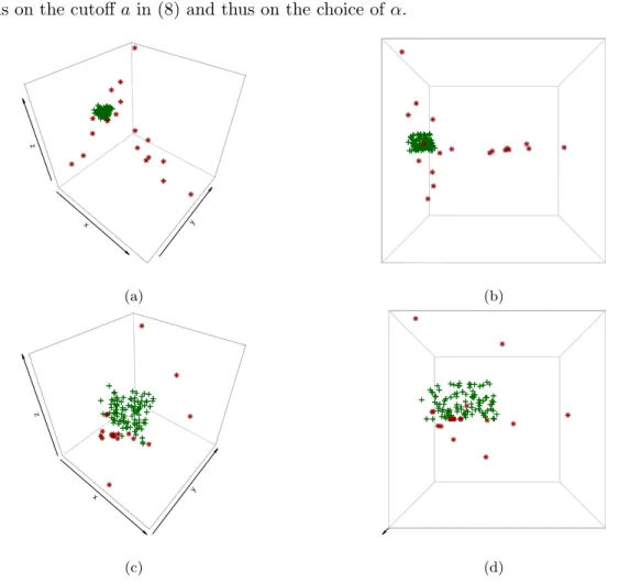
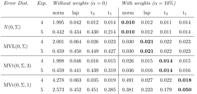
For centered observations, the diagnostic procedure with weights in (8) corresponds to a winsorization procedure which means that observations which lie far from the center are shrunken towards the center of the data. Figure 1 illustrates this idea for a three dimensional dataset. Figure 1 (a) shows the original dataset which contains some outlying observations that lie very far from the data center (i.e. the origin). The rotated view in Figure 1 (b) shows that the distance of the outlying points (red asterisks) is so large that it becomes impossible to distinguish the regular observations (green crosses) from each other. Applying the weighting procedure to reduce the effect of the most extreme observations, as described above, shrinks the most extreme outliers towards the origin. The outlying observations are thus brought closer to
the regular observations as can be seen from Figures 1 (c) and (d). The amount of shrinkage
depends on the cutoffain (8) and thus on the choice ofα.
x y z (a) x y z (b) x y z (c) x y z (d)
Fig. 1 (a) Original data points. (b) Rotated view which reveals the outliers even better. (c) Data points in space after applying the weighting procedure. (d) Rotated view after weighting.
The RBSUR model combines this diagnostic procedure with the robust procedure as
de-scribed earlier. LetW = diag(ω1, . . . , ωN) with ωi =ω(di) the weights given by (7)-(8), then
downweighting the leverage points transforms the data matrixZ intoZ? =W Z. The weighted
observationsz?i are thus given by
zi?= ((yi?)T,(x?i)T)T =ωizi = (ωiyiT, ωixTi )T, i= 1, . . . , N.
If this procedure has effectively reduced the effect of leverage points, then we can assume the SUR model for the weighted observations together with a heavy-tailed distribution for the errors.
Combining model (3) for the observations z?i with for example a Laplace distribution
MVL(0,Σ) for the errors?i =y?i −BTx?
i yields the likelihood
L(β,Σ|Z?)∝|Σ|−N/2 N Y i=1 exp − q (y?i −BTx? i) T Σ−1(y? i −BTx?i) . (9)
Note that this likelihood can be rewritten as L(β,Σ|Z?)∝ N Y i=1 ωiM|Σ|−1/2exp − q (yi−BTxi)TωiΣ−1ωi(yi−BTxi) ∝ N Y i=1 |(Σ/ωi2)|−1/2exp−q(y i−BTxi)T(Σ/ω2i)−1(yi−BTxi) . (10)
This formulation offers an alternative viewpoint on the RBSUR model as a SUR model with heteroscedastic errors. Within the high density region of the observations, it is assumed that
the SUR model holds with errors distributed according to MVL(0,Σ). This high density region
contains the observations zi with di ≤ a corresponding to ωi = 1. Outside the high density
region, the uncertainty on the SUR model is larger which is reflected by the increasing scale of
the error distribution. For these pointszithe error distribution is assumed to be MVL(0,Σ/ωi2)
with weight 0≤ωi <1. The weight function decreases to zero when the distancedi from the
center approaches infinity. However, it is important to stress that the weights ωi are used to
provide robustness against leverage points. Therefore, these weights are determined beforehand based on robust estimates of location and scatter which characterize the high density region, rather than estimating the weights simultaneously within the Bayesian estimation procedure. Remark that a similar derivation holds for the t-distribution.
3.3 Computation
We now discuss in detail how to perform inference in the RBSUR model. In the first step,
the weightsωi of the observations are calculated as explained earlier. Based on the weighted
observationsz?i the goal is then to obtain the posterior distribution
f(β,Σ|Z?)∝L(β,Σ|Z?)f(β,Σ) (11) of the model parameters. As for many Bayesian models, there exists no prior distribution for this model that leads to an analytical tractable posterior distribution. Therefore, a Markov Chain Monte Carlo (MCMC) sampler will be used to simulate the posterior distribution.
In the case of a normal likelihood function and conjugate priors, the conditional distributions
f(β|Σ, Z?) and f(Σ|β, Z?) can be easily derived. By exploiting these conditionals, the full
posterior distribution in (11) can be sampled by generating a Gibbs sequence. However, if the errors follow a heavy-tailed distribution like the Laplace distribution or t-distribution, then these conditionals cannot be computed analytically. To generate a Gibbs sequence for these error distributions, we will use the results on scale mixtures of multivariate normal distributions.
Let Z be a multivariate standard normal variable, i.e. Z ∼N(0, IM), and let V denote a
M and a positive definite matrix Σ of sizeM×M, the M-dimensional random variableU given by
U =µ+V−1/2Σ1/2Z, (12)
is said to have a scale mixture of multivariate normal distributions. The random variableV is
called the mixing variable. Now we will consider some specific choices forV. If V = 1, then
U ∼ N(µ,Σ). If the mixing variable follows an inverse gamma distribution IG(α1, α2) with
α1 = (M + 1)/2 and α2 = 1/2, then it can be proven that U follows a multivariate Laplace
distribution MVL(µ,Σ) (Arslan 2010). If the mixing variable follows a gamma distribution
G(α1, α2) withα1 =α2 =ν/2, then U follows a multivariate t-distribution MVt(µ,Σ, ν) with
ν degrees of freedom (Geweke 1993). Hence, the multivariate Laplace and the multivariate
t-distribution can be represented as a scale mixture of normal distributions. These properties can be exploited to bring the proposed model in the conjugate framework.
It follows from (12) that for a givenV =v, drawing from the correspondingU simplifies to
drawing from a multivariate normal distribution,
U|V =v ∼N(0,Σ/v).
Therefore, consideringV = (V1, . . . , Vn) as independent latent variables, the posterior density
becomes
f(β,Σ, v|Z?)∝L(β,Σ|v, Z?)f(β,Σ), (13)
withL(β,Σ|v, Z?) the likelihood function (Choi and Hobert 2013). However, we cannot observe
V in practice, so it needs to be estimated from the data. A Gibbs sequence can be created
to sample the posterior given in (13). The MCMC sampler thus cycles through the following three conditional distributions
f(β|Σ, v, Z?), f(Σ|β, v, Z?), f(v|β,Σ, Z?).
Draws from these conditionals will then form the marginal distributions ofβ and Σ.
To obtain the conditionals of β and Σ, we start by selecting a normal prior for β and
an inverse Wishart prior for Σ. These proper priors are conjugate with a normal likelihood. As in the Bayesian approach of Zellner (1996) we use vague priors. A normal prior is made vague by giving it a large variance (large determinant of the covariance matrix) and for the inverse Wishart prior, vagueness is achieved by choosing very small degrees of freedom. For the Bayesian SUR model it follows that
Using the scale transformations ˜yi?=vi1/2y?i and ˜x?i =vi1/2x?i, it equivalently holds that
˜
yi?|V =vi∼N(BTx˜?i,Σ).
The rescaled observations thus follow the standard SUR model with a normal likelihood. Since
the priorsβ∼N( ¯β,Γ¯−1) and Σ∼InvW(¯ν,∆) are conjugate for the normal likelihood, we can¯
obtain their conditional posterior distributions
β|Σ, v, Z?∼N(ˆΓ−1(¯Γ ¯β+ N X i=1 (X?i)T(Σ/vi)−1y?i),Γˆ−1), (14) with ˆΓ = ¯Γ + N X i=1 (X?i)T(Σ/vi)−1X?i, (15) and Σ|β, v, Z? ∼InvW(¯ν+n,∆)ˆ , (16) with ˆ∆ = ¯∆ + N X i=1 vi(yi?−X?iβ)(yi?−X?iβ)T = ¯∆ + N X i=1 vi(yi?−BTx?i)(yi?−BTx?i)T. (17)
As in Choi and Hobert (2013), it is also possible to derive the conditional distribution
f(v|β,Σ, Z?) for a specific error distribution. For Laplace distributions it can be shown that
the conditional distribution of Vi follows an inverse Gaussian distribution InvGaus(γi, λ = 1)
where γi = [(y−BTxi)TΣ−1(y−BTxi)]−1/2 (see e.g. Arslan (2010)). The inverse Gaussian
distribution is characterized by its density function given by
f(v;γ, λ) = λ 2πv3 1/2 exp −λ(v−γ)2 2γ2v .
For t-distributions withν degrees of freedom it can be shown that the conditional distribution
ofVifollows a gamma distribution G((ν+1)/2, αi) whereαi= ((y−BTxi)TΣ−1(y−BTxi)+ν)/2
(see e.g. Geweke (1993)).
For a Laplace likelihood the MCMC procedure can be summarized in the following steps.
1. For each observationzi compute its weightωi =w(di);
2. Calculate the weighted observationsz?i =ωizi;
3. Initializeβ and Σ by their prior modes:
4. For each of the observations, drawvi∼ InvGaus(γi,1) with ¯ γi = h (yi?−BTx?i)TΣ−1(yi?−BTx?i) i−1/2 ;
5. Drawβ from its conditional posterior distribution given by (14)-(15);
6. Draw Σ from its conditional posterior distribution given by (16)-(17); 7. Iterate steps 4 to 6.
If the likelihood is altered, the fourth step changes accordingly. Remark that the procedure holds for all distributions which can be represented as a scale mixture of normal distributions.
3.4 Robustness
Pe˜na et al. (2009) formalized robustness in the context of Bayesian inference by introducing
the concept ofα-robustness. A Bayesian inference method for a vector of parametersθis called
α-robust with respect to the Kullback-Leibler divergence if
sup Zα KL(Zα, Z) = Z log f(θ|Zα) f(θ|Z) f(θ|Zα)dθ <∞,
where f(θ|Z) and f(θ|Zα) are the posterior distributions for θ given the sample Z and Zα
respectively. The supremum is over all samples Zα that are obtained by replacing at most a
fraction α of the observations in the original sample Z by arbitrary outliers. The following
theorem whose proof is given in the Appendix shows that the Bayesian inference in the
RB-SUR model with multivariate Laplace distribution is α-robust. A similar result holds for the
multivariate t-distribution.
Theorem 1. Theorem 1. LetZ = (z1, . . . , zn)T withzi = (yiT, xTi )T be an(M+p)-dimensional
dataset of sizeN withd(1−α)Ne> M+p, which is in general position (i.e. any affine subspace
of dimensionM+p−1contains at mostM+pobservations). If the posterior distribution in the
RBSUR model with likelihood given by (9) is proper such that the Kullback-Leibler divergence
exists, then the Bayesian inference is α-robust with respect to the Kullback-Leibler divergence
for 0< α <1/2.
In the next sections, the applicability of the method is shown on simulated datasets as well as real-life data.
4
SIMULATIONS
In this section we assess the performance of the Robust Bayesian SUR model. First, we
evaluate the MCMC procedure to obtain the posterior distributions of the model parameters. We take the mean of the posterior distributions, i.e. the Bayes estimates, as the estimators of the parameters. We investigate the performance of the estimators in the SUR model with multivariate Laplace and Student’s t errors. This shows how effective the Bayesian inference is under ideal circumstances. In the second part we then evaluate the robustness of the estimator by generating data from other models.
4.1 RBSUR performance
We consider the SUR model of Section 2 with M = 2 blocks and N = 100 observations in
each block. The errors i are first generated from a bivariate Laplace distribution and then
from a bivariate t-distribution with 3 degrees of freedom. In both cases the error distribution is centered at zero and has scatter matrix
Σ = 1 0.5 0.5 1 . (18)
Both regression equations contain two covariates. The first covariate is the constant 1 to include an intercept in the models while the second covariate is generated from a standard
normal distribution in both cases. The regression coefficients are set equal to β1 = (1,−1)T
andβ2 = (−1,1)T respectively. The corresponding responses are obtained from (1) so that the
data follow the SUR model with either multivariate Laplace or Student’s t errors. We apply
our Bayesian estimation to these data without applying any weighting (α= 0). The MCMC is
run with 5000 iterations and diffuse priors are used as follows. The prior forβ = (β1T, β2T)T is a
multivariate normal distribution with mean zero, variances equal to 100 and zero correlations.
For Σ we have used an inverse Wishart prior with a small (¯ν =M+ 1 = 3) degrees of freedom
and scale matrix equal to the bivariate identity matrix. These priors are vague, but the sampler is still able to approximate well the posterior distribution, with good convergence properties. We have also experimented with non-informative priors, i.e. infinite variances for the regression coefficients and zero degrees of freedom for the Wishart prior. The non-informative priors yield similar results as the vague priors, therefore we do not report these results.
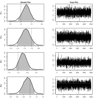
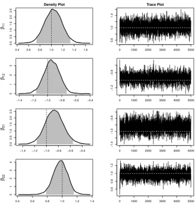
Figures 2 and 3 show the posterior distributions of the regression coefficients for
respec-tively the Laplace distribution and the t3-distribution. Kernel density estimates of the
0.5 1.0 1.5 2.0 0.0 0.5 1.0 1.5 2.0 Density Plot β11 0 1000 2000 3000 4000 5000 0.6 1.0 1.4 1.8 Trace Plot −1.6 −1.4 −1.2 −1.0 −0.8 0.0 1.0 2.0 3.0 β12 0 1000 2000 3000 4000 5000 −1.6 −1.2 −0.8 −1.5 −1.0 −0.5 0.0 0.0 0.5 1.0 1.5 2.0 β21 0 1000 2000 3000 4000 5000 −1.0 −0.5 0.0 0.4 0.6 0.8 1.0 1.2 1.4 0.0 1.0 2.0 3.0 β22 0 1000 2000 3000 4000 5000 0.4 0.6 0.8 1.0 1.2
Fig. 2Marginal posterior density plots and trace plots for the regression coefficients β11, β12,β21 and β22in case of data with bivariate Laplace errors. The vertical and horizontal dashed lines represent the trueβ values. Gray zones on the density plots mark 95% credible intervals.
the right. The dashed line in each of these plots indicates the corresponding true value of
β = (β11, β12, β21, β22)T. The trace plots show that the MCMC mixes very well. The effect
of the starting values for β and Σ disappears quickly. The shaded area in the density plots
represents the 95% credible interval corresponding to the posterior distribution. The true pa-rameter value lies well within its credible interval in all cases. The results in Figures 2 and 3 offer a clear indication of good performance of our Bayesian method under ideal conditions.
4.2 Robustness
We now investigate the robustness of the RBSUR and make a comparison with the standard Bayesian SUR model. To investigate the robustness, we simulate data with different data generating processes resulting in deviations from the classical assumptions of the SUR model. Five different data generating processes and four different error distributions are investigated.
We again consider a SUR model withM = 2 regression equations and two covariates in each
equation. One covariate corresponds to the intercept, while the second covariate is generated
from a standard normal distribution. The sample size in each block isN = 100. To generate
0.4 0.6 0.8 1.0 1.2 1.4 1.6 0.0 0.5 1.0 1.5 2.0 2.5 Density Plot β11 0 1000 2000 3000 4000 5000 0.6 1.0 1.4 Trace Plot −1.4 −1.2 −1.0 −0.8 −0.6 −0.4 0 1 2 3 β12 0 1000 2000 3000 4000 5000 −1.2 −0.8 −1.4 −1.2 −1.0 −0.8 −0.6 −0.4 0.0 0.5 1.0 1.5 2.0 2.5 β21 0 1000 2000 3000 4000 5000 −1.4 −1.0 −0.6 0.4 0.6 0.8 1.0 1.2 1.4 0 1 2 3 4 β22 0 1000 2000 3000 4000 5000 0.6 0.8 1.0 1.2
Fig. 3Marginal posterior density plots and trace plots for the regression coefficients β11, β12,β21 and β22 in case of data with bivariatet3 errors. The vertical and horizontal dashed lines represent the true
β values. Gray zones on the density plots mark 95% credible intervals.
and MVt(0,Σ,3) with scatter matrix Σ given in (18).
The first experiment uses uncontaminated data which fulfill all model assumptions of the
SUR model. The regression coefficients equalβ1 = (1,−1)T andβ2= (−1,1)T as before, which
implies that
yi∼N(Xiβ,Σ) =N((xT1iβ1, xT2iβ2)T,Σ),
if the errors are normally distributed and similarly for other error distributions. In the second experiment the response is contaminated for 5% of the observations. For both equations the
contaminated responses are generated according toN(20,1). In the third experiment 5% of the
observations are contaminated in both the response and the regressors. To this end, the data are generated as in the first experiment, but then the values of the second predictor variable (i.e. the intercept remains unchanged) in both regression equations are replaced by values from
a N(10,1) distribution for 5% of the observations. This produces bad leverage points. The
fourth and fifth experiment are the same as experiment two and three respectively, but with 10% of outlying observations.
The five data generating processes are repeated 1000 times. For each simulated dataset
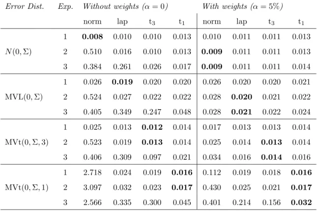
Table 1MSE of BSUR and RBSUR with and without weights for errors generated from the multivariate normal, Laplace distribution, t3 or Cauchy distribution, all with scatter matrix Σ as given in (18). RBSUR uses the normal (norm), Laplace (lap), multivariate t3 (t3) or Cauchy (t1) likelihood. Data
contain either no outliers (Exp. 1) or 5% of contamination which are outliers in the response variable (Exp. 2) or bad leverage points (Exp. 3). For each simulation setting (i.e. each row in the tables) the lowest MSE is highlighted in bold.
Error Dist. Exp. Without weights (α= 0) With weights (α= 5%)
norm lap t3 t1 norm lap t3 t1
N(0,Σ) 1 0.008 0.010 0.010 0.013 0.010 0.011 0.011 0.013 2 0.510 0.016 0.010 0.013 0.009 0.011 0.011 0.013 3 0.384 0.261 0.026 0.017 0.009 0.011 0.011 0.014 MVL(0,Σ) 1 0.026 0.019 0.020 0.020 0.026 0.020 0.020 0.021 2 0.524 0.027 0.022 0.022 0.028 0.020 0.021 0.022 3 0.405 0.349 0.247 0.048 0.028 0.021 0.022 0.024 MVt(0,Σ,3) 1 0.025 0.013 0.012 0.014 0.017 0.013 0.013 0.014 2 0.523 0.019 0.013 0.014 0.025 0.014 0.013 0.014 3 0.406 0.309 0.097 0.021 0.034 0.016 0.014 0.016 MVt(0,Σ,1) 1 2.718 0.024 0.019 0.016 0.112 0.019 0.018 0.016 2 3.097 0.032 0.023 0.017 0.430 0.025 0.021 0.017 3 2.566 0.335 0.300 0.045 0.401 0.214 0.156 0.032
10%) and without weights (α = 0). Moreover, four different likelihoods are considered for
RBSUR: normal, Laplace, multivariate Cauchy (i.e. multivariate t with 1 degree of freedom) and multivariate t with 3 degrees of freedom. Note that the choice of the likelihood determines step 4 of the algorithm in Subsection 3.3. Remark that in case a normal likelihood is used without weights, RBSUR coincides with the standard BSUR. As before, the MCMC is run with 5000 iterations and diffuse priors are used. The Bayesian estimates are computed as the mean of the marginal posterior distributions, i.e. the so-called Bayes estimate. We compare the
methods by calculating the mean squared error of the estimators of the regression coefficientsβ
based on the 1000 generated datasets for each setting. These results are summarized in Table 1 for the first three experiments (Exp. 1-3) and in Table 2 for the last two experiments (Exp. 4 and 5) with 10% of contamination.
When all the data follow the SUR model as in experiment one, then we can see from the first row in Table 1 that the performance of all estimators is similar. The standard BSUR (i.e.
Table 2MSE of BSUR and RBSUR with and without weights for errors generated from the multivariate normal, Laplace distribution, t3 or Cauchy distribution, all with scatter matrix Σ as given in (18). RBSUR uses the normal (norm), Laplace (lap), multivariate t3 (t3) or Cauchy (t1) likelihood. Data
contain 10% of contamination which are outliers in the response variable (Exp. 4) or bad leverage points (Exp. 5). For each simulation setting (i.e. each row in the tables) the lowest MSE is highlighted in bold.
Error Dist. Exp. Without weights (α = 0) With weights (α= 10%)
norm lap t3 t1 norm lap t3 t1
N(0,Σ) 4 1.995 0.042 0.012 0.014 0.010 0.012 0.011 0.014 5 0.442 0.434 0.430 0.214 0.010 0.012 0.011 0.014 MVL(0,Σ) 4 2.001 0.064 0.026 0.023 0.030 0.021 0.022 0.023 5 0.459 0.450 0.449 0.427 0.030 0.021 0.022 0.023 MVt(0,Σ,3) 4 1.998 0.046 0.016 0.015 0.026 0.015 0.014 0.015 5 0.459 0.441 0.439 0.319 0.036 0.016 0.014 0.016 MVt(0,Σ,1) 4 4.278 0.063 0.035 0.019 0.491 0.027 0.022 0.018 5 2.573 0.452 0.451 0.385 0.381 0.223 0.179 0.050
normal likelihood without weights) performs slightly better than the robust methods. However, this reverses when the data follow other error distributions. In particular, it is clear that BSUR cannot handle Cauchy errors. The standard BSUR also does not perform well on data with outlying responses (Exp. 2 and 4), but the RBSUR methods with heavy-tailed likelihoods perform much better, even without weights. Adding weights only slightly decreases their MSE, confirming that using a heavy-tailed likelihood suffices to handle a fraction of vertical outliers. Remark also that the performance is nearly the same for all three heavy-tailed likelihoods, indicating that the RBSUR method is not sensitive to the choice of the heavy-tailed distribution for the errors. Adding weights to the standard BSUR also greatly improves its performance on data with response outliers. However, when the error distribution is extreme (Cauchy errors) then BSUR with weights and normal likelihood still performs worse than the RBSUR methods with heavy-tailed likelihood. When the data contain bad leverage points (Exp. 3 and 5), then RBSUR with weights becomes the preferred model. While the MSE of BSUR increases dramatically in this case, the MSE of RBSUR with weights remains stable, confirming that the bad leverage points have little effect on these methods. From the results in Table 1 (Exp. 3) we can see that even without weights RBSUR with Cauchy likelihood can cope quite well with 5% of bad leverage points, but this is not true anymore when the contamination fraction increases to 10% as seen from Table 2 (Exp. 5).
5
REAL DATA EXAMPLE
To illustrate the RBSUR method, we consider Grunfeld’s dataset (Grunfeld 1958) which has been used several times as a SUR example (see Bilodeau and Duchesne 2000, and references therein). This dataset contains data from 10 U.S. corporations for the period 1935-1954. The value of outstanding shares and capital stock at the beginning of the year as well as their annual gross investment is recorded for each of the 10 corporations for all 20 consecutive years. The aim is to investigate how well capital stock (Capital) and the outstanding shares (Value) explain the variations in annual gross investment. Since general economic factors may affect all firms contemporaneously, errors may be correlated which makes the SUR model appropriate. To be able to compare our method to the results of Bilodeau and Duchesne (2000), we analyze the data of the two energy corporations, General Electric and Westinghouse. Consequently, the SUR model is given by
Investmentmi=βm0+βm1Valuemi+βm2Capitalmi+mi,
with Cov (mi, m0i) =σmm0 fori= 1, . . . ,20 andm, m0 = 1,2.
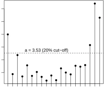
In the first step, we screen the data for possible outliers by calculating the distances di
of the observations as given by (7). The resulting distances are shown in Figure 4. From
● ● ● ● ● ● ● ● ● ● ● ● ● ● ● ● ● ● ● ● 2 3 4 5 6 7 year distance 1935 1936 1937 1938 1939 1940 1941 1942 1943 1944 1945 1946 1947 1948 1949 1950 1951 1952 1953 1954 a = 3.53 (20% cut−off)
Fig. 4 Observations (years) and their robust distances from the data center. The horizontal dashed line represents the cut-off forα= 20%.
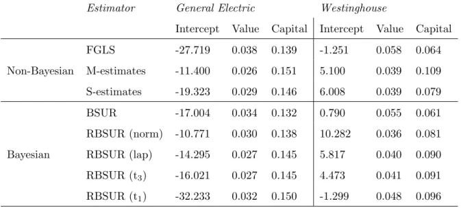
Table 3 Estimates of the regression parameters in Grunfeld’s data example. RBSUR is applied with four different likelihoods: normal (norm), Laplace (lap), Student’s t with 1 degree of freedom (t1) and
Student’s t with 3 degrees of freedom (t3).
Estimator General Electric Westinghouse
Intercept Value Capital Intercept Value Capital
Non-Bayesian FGLS -27.719 0.038 0.139 -1.251 0.058 0.064 M-estimates -11.400 0.026 0.151 5.100 0.039 0.109 S-estimates -19.323 0.029 0.146 6.008 0.039 0.079 Bayesian BSUR -17.004 0.034 0.132 0.790 0.055 0.061 RBSUR (norm) -10.771 0.030 0.138 10.282 0.036 0.081 RBSUR (lap) -14.295 0.027 0.145 5.817 0.040 0.090 RBSUR (t3) -16.021 0.027 0.145 4.473 0.041 0.091 RBSUR (t1) -32.233 0.032 0.150 -1.299 0.048 0.096
years (1952-1954) and the first year (1935), while the observations in the remaining period (1936-1951) lie closer together. Note that these four years were also identified by the analysis of Bilodeau and Duchesne (2000) who relate them to economical evaluations such as the postwar
booming economy for the years 1952-1954. Therefore, we apply RBSUR with α= 20% which
corresponds to downweighting four outliers as can be seen from Figure 4.
In Table 3 the parameter estimates obtained by RBSUR (taken as the marginal means of 5000 MCMC runs with vague priors) are compared to the estimates obtained by the non-robust feasible generalized least squares (FGLS) and BSUR methods as well as to the robust estimates obtained by Bilodeau and Duchesne (2000) for the S-estimator and the M-estimator (Koenker and Portnoy 1990). The non-robust BSUR, and FGLS estimators yield similar estimates for the effects of Value and Capital, while the intercept shows more difference. Also for the robust methods, there is considerable variation in the intercept. However, the robust estimators con-sistently estimate a smaller effect for Value and a larger effect for Capital. The estimated slopes are similar for all robust methods. The RBSUR slope estimates are closer to the more robust S-estimates than to the M-estimates which cannot withstand high leverage points. Remark also that the RBSUR estimates based on Laplace likelihood and Student’s t likelihood with 3 degrees of freedom are almost identical.
Figure 5 compares the marginal posterior distributions of the SUR parameters. The stan-dard BSUR model is compared to the RBSUR model with Laplace likelihood with varying degrees of shrinkage. For clarity of exposition, the posteriors of the other fat-tailed likelihoods
−100 −50 0 50 0.000 0.010 0.020 intercept GE Density SUR lapSUR lapSUR10 lapSUR20 −0.02 0.00 0.02 0.04 0.06 0.08 0 10 20 30 40 value GE Density SUR lapSUR lapSUR10 lapSUR20 0.00 0.05 0.10 0.15 0.20 0 5 10 15 20 capital GE Density SUR lapSUR lapSUR10 lapSUR20 −30 −20 −10 0 10 20 30 0.00 0.02 0.04 0.06 0.08 intercept WH Density SUR lapSUR lapSUR10 lapSUR20 0.00 0.02 0.04 0.06 0.08 0.10 0 10 20 30 40 value WH Density SUR lapSUR lapSUR10 lapSUR20 −0.1 0.0 0.1 0.2 0.3 0 2 4 6 8 10 capital WH Density SUR lapSUR lapSUR10 lapSUR20
Fig. 5Comparison of the marginal posterior distributions for the Bayesian SUR model and the proposed robust model with Laplace likelihood with varying levels ofα={0.0,0.1,0.2}.
are omitted. Nevertheless, the resulting graphs are very similar to the ones in Figure 5. The fig-ure shows how for some parameters (e.g. intercept GE) the robust procedfig-ure only has minimal influence on the marginal posterior, while for other parameters the impact is more pronounced (e.g. intercept WH). Also notice how the modes of the marginal posteriors are sometimes pulled towards zero (e.g. value WH) or sometimes pulled away from zero (e.g. intercept WH) depend-ing on the location of the outliers with respect to the bulk of the data. Together with this location shift, the proposed approach also increases the variance of the marginal posterior.
These effects vary with the different levels ofα.
model (taken as the marginal means of 5000 MCMC runs with vague priors). Our main interest
is on the correlation corresponding to the covariance σ12. In absence of correlation, it is not
necessary to fit a SUR model, and the two regression equations can be analyzed separately. The
non-robust FGLS and BSUR estimate this correlation to be 0.77 and 0.75, respectively. These
correlation estimates indicate that the SUR model is indeed needed to take correlation among the errors into account. However, since there are outliers in the data that potentially influence these estimates, we now examine the robust estimates of the correlation. The M-estimator
of (Koenker and Portnoy 1990) yields 0.73, the S-estimator of Bilodeau and Duchesne (2000)
yields 0.85, and forα= 20% the RBSUR estimates are 0.82,0.80,0.79 and 0.75 for respectively
normal, Laplace,t3 and Cauchy likelihoods. These results show that the outliers do not distort
the correlation among the errors and the SUR model is really needed to analyze the data.
6
DISCUSSION
In this paper a Robust Bayesian SUR model is developed. Heavy tails in the error distribu-tion are tolerated by using a multivariate Laplace distribudistribu-tion or a multivariate t-distribudistribu-tion. Moreover, leverage points are handled effectively by downweighting the most scattered obser-vations in the likelihood. An efficient Gibbs sampler has been worked out by exploiting the fact that these heavy-tailed distributions can be represented as a mixture of normals, so that con-jugate priors could be used. An empirical analysis revealed that the RBSUR method remains close to the standard Bayesian SUR under ideal conditions while RBSUR clearly outperforms the BSUR model for contaminated data.
The focus of the manuscript is on parameter estimation and as such prediction or model se-lection are not explicitly discussed. As the posterior of the models proposed in this manuscript is not analytically tractable, the posterior predictive distribution or marginal likelihood are neither. Nevertheless, given a sample of draws from the posterior distribution, the posterior predictive distribution or the Bayes Factor can be simulated using standard approaches (Gel-man et al. 2015). However, note that for Bayes Factor approximations, the vague priors used in the data examples are suboptimal and more informative priors should be used.
The robustness of the approach, formally shown by the α-robustness of the method, is
determined by the maximally tolerable contamination fractionα which is a tuning parameter
that needs to be chosen by the user. If the fraction α is chosen too small, then some leverage
points will not be downweighted and may have a high impact on the resulting estimates,
leading to an undesirable result. On the other hand, if α is chosen very large, then even
is well-known in robustness (see e.g. Maronna et al. 2006) and can even be intertwined with other tuning parameters in complex settings such as clustering (Garc´ıa-Escudero et al. 2011). Diagnostic procedures such as the plot of the observation distances in Figure 4 are useful to
guide the user in his choice ofα.
We have not formally shown that RBSUR inference yields a genuine posterior distribution.
As shown by Pe˜na et al. (2009) a likelihood formed as the product of independent
observa-tions with a common density is generally not α-robust. However, the RBSUR likelihood (10)
corresponds to a SUR model with heteroscedastic errors. If the diagnostic procedure in Sub-section 3.2 consistently estimates the weights of the heteroscedastic SUR model, then it may be feasible to establish that the RBSUR asymptotically yields the same posterior distribution corresponding as the genuine likelihood of the heteroscedastic SUR model by using similar techniques as in Greco et al. (2008) and Agostinelli (2013). This will be investigated in further research.
References
Agostinelli C, Greco L (2013) A weighted strategy to handle likelihood uncertainty in bayesian inference. Comput Stat 28:319–339
Ando T (2011) Bayesian Variable Selection for the Seemingly Unrelated Regression Models with a Large Number of Predictors. J Japan Statist Soc 41:187–203
Ando T, Zellner A (2010) Hierarchical bayesian analysis of the seemingly unrelated regression and simultaneous equations models using a combination of direct monte carlo and importance sampling techniques. Bayesian Anal 5:65–95
Andrade J A A, O’Hagan A (2006) Bayesian robustness modeling using regularly varying distributions. Bayesian Anal 1:169–188
Arslan O (2010) An alternative multivariate skew Laplace distribution: properties and estima-tion. Statist Papers 51:865–887
Bayarri M, Morales J (2003) Bayesian measures of surprise for outlier detection. J Statist Plann Inference 111:3–22
Benoit D F, Van Aelst S, Van den Poel D (2015) Outlier-Robust Bayesian Multinomial Choice Modeling. J Appl Econ 31:1445–1466
Billio M, Casarin R, Rossini L (2016) Bayesian nonparametric sparse seemingly unrelated regression model (SUR). Working Papers 2016:20, Department of Economics, University of Venice “Ca’ Foscari”
Bilodeau M, Duchesne P (2000) Robust estimation of the SUR model. Can J Stat 28:277–288 Chib S, Greenberg E (1995) Hierarchical analysis of sur models with extensions to correlated
serial errors and time-varying parameter models. J Econ 68:339–360
Choi H M, Hobert J P (2013) Analysis of MCMC algorithms for Bayesian linear regression with Laplace errors. J Multivariate Anal 117:32–40
Farcomeni A, Greco L (2015) Robust Methods for Data Reduction. Chapman and Hall–CRC
Garc´ıa-Escudero L, Gordaliza A, Matr´an C, Mayo-Iscar A (2011) Exploring the number of
groups in robust model-based clustering. Stat Comput 21:585–599
Gelman A, Carlin J B, Stern H, Dunson D, Vehtari A, Rubin D (2015) Bayesian Data Analysis, 3rd edition. Chapman and Hall–CRC
Geweke J (1993) Bayesian Treatment of the Independent Student-t Linear Model. Appl Econ 8:19–40
Greco L, Racugno W, Ventura L (2008) Robust likelihood functions in bayesian inference. J Statist Plann Inference 138:1258–1270
Grunfeld Y (1958) The Determinants of Corporate Investment. PhD thesis, Department of Economics, University of Chicago
Hubert M, Rousseeuw P J, Van Aelst S (2008) High-breakdown robust multivariate methods. Statist Sci 23:92–119
Koenker R, Portnoy S (1990) M-estimation of multivariate regressions. J Amer Statist Assoc 85:1060–1068
Kotz S, Kozubowski T, Podgorski K (2001) The Laplace distribution and generalizations: a revisit with applications to communications, economics, engineering, and finance. Springer Science & Business Media
Lavine M (1991) Sensitivity in bayesian statistics: The prior and the likelihood. J Amer Statist Assoc 86:396–399
Lavine M (1994) An approach to evaluating sensitivity in bayesian regression analyses. J Statist Plann Inference 40:233–244
Maronna R A, Martin D R, Yohai V J (2006) Robust Statistics: Theory and Methods. Wiley, New York
Ng V M (2002) Robust bayesian inference for seemingly unrelated regressions with elliptical errors. J Multivariate Anal 83:409–414
Pe˜na D, Zamar R, Yan G (2009) Bayesian likelihood robustness in linear models. J Statist
Plann Inference 139:2196–2207
Peremans K, Van Aelst S (2018) Robust inference for seemingly unrelated regression models. J Multivariate Anal 167:212–224
Sivaganesan S (1993) Robust bayesian diagnostics. J Statist Plann Inference 35:171–188 Train K (2003) Discrete Choice Methods with Simulation. Cambridge University Press:
Cam-bridge, UK
Verzilli C J, Stallard N, Whittaker J C (2005) Bayesian Modelling of Multivariate Quantitative Traits Using Seemingly Unrelated Regressions. Genet Epidemiol 28:313–325
Watson J, Holmes C (2016) Approximate models and robust decisions. Statist Sci 31:465–489 Zellner A (1962) An efficient method of estimating seemingly unrelated regressions and tests
for aggregation bias. J Amer Statist Assoc 57:348–368
Zellner A (1996) An Introduction to Bayesian Inference in Econometrics. Wiley
Zellner A, Ando T (2010a) Bayesian and non-bayesian analysis of the seemingly unrelated regression model with student-t errors, and its application for forecasting. Int J Forecast 26:413–434. Special Issue: Bayesian Forecasting in Economics.
Zellner A, Ando T (2010b) A direct monte carlo approach for bayesian analysis of the seemingly unrelated regression model. J Econ 159:33–45
A
APPENDIX
Theorem 1. We follow the lines of the proof of Theorem 2 in Pe˜na et al. (2009). This means that
we have to show that the weighted observationsz?
i are bounded which implies that the
of the observations, Z can be split into Z = Z1
Z2
. Z1 contains the d(1−α)ne observations
that remain uncontaminated inZα, whileZ2 contains the remaining [αn] observations that are
replaced by outliers inZα. The contaminated dataZα can similarly be split intoZα=
Z 1 Z2,α . Moreover, denote Z?
α = W Zα with W = diag(ω1, . . . , ωN) and ωi = ω(di) with di = di(Zα)
given by (7).
We first show that the constantawhich is the (1−α) quantile of the distancesdiis bounded.
Sinceα <1/2 and the coordinate-wise medianT and the scatter matrixCboth have breakdown
point 1/2 under the conditions of the theorem, there exist bounds BT(Z1) and Bl(Z1) such
thatkT(Zα)k ≤BT(Z1)k<∞ and 0< Bl(Z1)≤λmin(C(Zα))≤λmax(C(Zα))≤Bu(Z1)<∞
whereλmin(C(Zα)) and λmax(C(Zα)) are the smallest/largest eigenvalue ofC(Zα). For every
zα,i inZα it then follows that
kzα,i−T(Zα)k/ p
Bu(Z1)≤di ≤ kzα,i−T(Zα)k/ p
Bl(Z1)
For observations zα,i in Z1, we have that zα,i = zi and the corresponding distances di have
a finite lower and upper bound that only depends on Z1. This implies immediately that the
(1−α) quantile of the distancesdi inZα is bounded (and positive) whatever the outliers are.
Now, consider zi? =ωizα,i. If di > a, then we have that
d?i = q (z? i −T)TC−1(zi?−T) ≤ q (z?i −ωiT)TC−1(z?i −ωiT) + (1−ωi) √ TTC−1T ≤di(1 +d2i −a2)−1/2+kTk/ p Bl(Z1) ≤max(1, a) +BT(Z1)/ p Bl(Z1),
which is bounded. If di ≤ a, then ωi = 1 and thus di? = di ≤ a. Hence, d?i has a finite
upper bound for all observations in Zα and thus also kz?ik has a finite upper bound for the