a dissertation
submitted to the faculty of the graduate school
of the university of minnesota
by
Subhabrata Majumdar
in partial fulfillment of the requirements
for the degree of
doctor of philosophy
Snigdhansu Chatterjee, Adviser
- Issac Newton
Simplicity is the final achievement. After one has played a vast quantity of notes and more notes, it is simplicity that emerges as the crowning reward of art.
- Fr´ed´eric Chopin
c
I would like to thank my advisor, Prof. Snigdhansu Chatterjee for everything he has done for me. This dissertation would not have been possible without the very fundamental ideas behind it that came out of our discussions during the first two years of my PhD. Anshu da gave me the freedom to pursue those ideas and shape them as I wanted. I am thankful for the professional support he provided, as well as for always being available to listen to my ramblings. I am going to miss those weekly meetings in which we talked about anything and everything statistics.
I want to thank Prof. Saonli Basu of the Division of Biostatistics, with whom I collaborated during my last year. She has been an invaluable mentor, and discussions with her helped me learn about many applied aspects of the problems we had worked on. Thanks to her for being a reviewer of this dissertation as well. Special thanks to Profs. Lan Wang and Xiaotong Shen for reviewing the thesis and being on the final exam committee, and Prof. Gongjun Xu for being in my oral committee.
I would like to thank other professors in the department, who have always been helpful in answering questions, and the staff in the department office for their support regarding official matters. Thanks to other students in the department, for being there with feedback and discussions: especially Abhirup, Adam, Aaron, Daniel, Dootika and Sakshi.
I would like to acknowledge the National Science Foundation Climate Expeditions grant IIS-1029711, which provided me funding for 3 semesters, and the University of Minnesota Graduate School’s Interdisciplinary Doctoral Fellowship (IDF), which supported me during my final year.
I consider myself very fortunate to have worked with a number of collaborators
while still being a graduate student. Thanks to Profs. Matt McGue and Mike Miller of the Department of Psychology for their help during the IDF collaboration. Out-side the campus, I am grateful to Prof. Subhash C. Basak of University of Minnesota Duluth for helping me write my first paper back in 2012 and all subsequent collabo-rations. Rayid Ghani of University of Chicago and Kush Varshney of IBM Research have been inspirations in developing my approach to collaborative research.
Coming to personal life, I would like to thank my friends for keeping me grounded and connected to the world outside. Special thanks to the three musketeers- Abhirup Mallik, Somnath Kundu and Suvankar Biswas, for being part of many happy memories during the past five years. I am grateful to Abhishek Nandy, for all his support during my first two years. Thanks to Amit da, Arja, Deepashree, Shriya, Tallin di, Taraswi di, Tushar and many more people associated with the Bengali Student Society of Minnesota, life in Minneapolis has been so much enjoyable.
I would like to thank my teachers from school, Prabhat Kusum Sarkar for intro-ducing me to statistics, and Tapas Kumar Dhar for helping me build the necessary mathematical foundation. The past five years would not have been possible without the all-encompassing influence of Indian Statistical Institute (ISI), where I finished my bachelors and masters degree. This is too short a space to list all the avenues the ISI connection has helped me through in terms of personal and professional networking. I am thankful for being part of this ISI family.
Finally, I want to thank the three people closest to me for always being there no matter what. My girlfriend, Rajeshwaree Chatterjee, has been a constant source of motivation and fresh perspectives on life, even from half a world away in Kolkata. To the other two persons, my parents, I owe more than anyone else in this world. In spite of coming from humble beginnings, they have the highest respect for the intellectual pursuit, and there is no substitute for the sacrifices they made in bringing me up. Ma and Baba, I dedicate this thesis to you.
This dissertation is dedicated to my parents:
Samita Mazumder, my mother- for being patient while teaching a little boy the al-phabets of mathematics, and instilling in me the value of hard work; and
Satyabrota Mazumder, my father- for the many life lessons, and wholeheartedly sup-porting me in every major decision I have made.
Data depth provides a plausible extension of robust univariate quantities like ranks, order statistics and quantiles in multivariate setup. Although depth has gained visi-bility and has seen many applications in recent years, especially in classification prob-lems for multivariate and functional data, its generalizability and utility in achieving traditional parametric inferential goals is largely unexplored. In this thesis we de-velop several approaches to address this. In particular, firstly we define an evaluation map function that is more general than data depth, and establish several results in a parametric modelling context using a broad definition of a statistical model. A fast algorithm for covariate selection using data depths as evaluation functions arises as a special case of this. We demonstrate applications of this framework on data from diverse fields: namely climate science, medical imaging and behavioral genetics. Sec-ondly we propose a multivariate rank transformation using data depth and use them for robust inference in location and scale problems in elliptical distributions. Thirdly, we lay out a depth-based regularization framework in multi-response regression, and derive a new method of nonconvex penalized sparse regression in the multitask situa-tion. Across the thesis, several simulation studies and real data examples demonstrate the effectiveness of the methods developed here.
List of Tables ix
List of Figures xi
List of Notations xiii
1 Introduction 1
1.1 Background . . . 1
1.2 Definition and examples . . . 2
1.3 Why is depth not a thing yet? . . . 4
1.4 Summary of work . . . 5
2 Generalized Model Discovery using Statistical Evaluation Maps 8 2.1 Introduction . . . 8
2.2 The general framework . . . 14
2.2.1 The frame of models . . . 14
2.2.2 Transformation to a common platform . . . 16
2.2.3 Method of estimation . . . 19
2.3 Statistical evaluation maps ande-values . . . 22
2.3.1 A general evaluation map . . . 22
2.3.2 The e-value of models . . . 23
2.3.3 Model adequacy and e-values . . . 24
2.4 Estimation of e-values through resampling . . . 26
2.4.1 Smooth estimating functional models . . . 27
2.4.2 Bootstrap estimation of e-values . . . 32
2.5 Fast variable selection using data depth . . . 33
2.5.1 A plugin parameter estimate . . . 34
2.5.2 Simplifications . . . 35
2.5.3 Derivation of the algorithm . . . 38
2.5.4 Bootstrap implementation . . . 40
2.6 Simulation studies . . . 42
2.6.1 Selecting covariates in linear regression . . . 43
2.6.2 Model selection in the presence of random effects . . . 47
2.7 Discussion and conclusion . . . 49
2.8 Proofs . . . 51
3 Applications of the Evaluation Maps Framework 65 3.1 Identifying Driving Factors Behind Indian Monsoon Precipitation . . 65
3.2 Spatio-temporal Dependence Analysis in fMRI data . . . 70
3.2.1 Temporal model . . . 70
3.2.2 Spatial model . . . 71
3.3 Selection of Important Single Nucleotide Polymorphisms behind be-havioral traits from Familial Genome Wide Association Studies data . 74 3.3.1 Motivation . . . 74
3.3.2 The MCTFR data . . . 76
3.3.3 Statistical model . . . 77
3.3.4 A conditional e-value . . . 79
3.3.5 Simulation . . . 84
3.3.7 Future work: incorporating group selection for GWAS . . . 96
4 Signed Peripherality Functions in Multivariate Analysis 98 4.1 Introduction . . . 98
4.2 The robust location problem . . . 100
4.2.1 The weighted spatial median . . . 102
4.2.2 A high-dimensional test of location . . . 104
4.3 Depth-based rank covariance matrix . . . 106
4.3.1 Calculating the sample DCM and ADCM . . . 110
4.3.2 Robust PCA using eigenvectors of DCM . . . 113
4.4 Robust PCA and supervised models . . . 125
4.5 Robust inference with functional data . . . 127
4.6 Conclusion . . . 131
4.7 Appendix . . . 132
4.7.1 Form of ˜VpFq . . . 132
4.7.2 Asymptotics of eigenvectors and eigenvalues . . . 133
4.7.3 Proofs . . . 136
5 Nonconvex Penalized Regression using Depth-based Penalty 142 5.1 Introduction . . . 142
5.2 Depth-based regularization . . . 145
5.3 The LARN algorithm . . . 146
5.3.1 Formulation . . . 146
5.3.2 The one-step estimate and its oracle properties . . . 150
5.3.3 Recovering sparsity within a row . . . 151
5.3.4 Computation . . . 152
5.4 Orthogonal design and independent responses . . . 154
5.4.2 Minimax optimal performance . . . 156
5.5 Simulation results . . . 157
5.5.1 Methods and setup . . . 157
5.5.2 Evaluation . . . 158
5.6 Real data example . . . 161
5.7 Conclusion . . . 163
5.8 Proofs . . . 163
6 Future Work 169 6.1 Characterization of depth in general normed spaces . . . 169
6.2 Future of e-values . . . 170
6.3 Others . . . 170
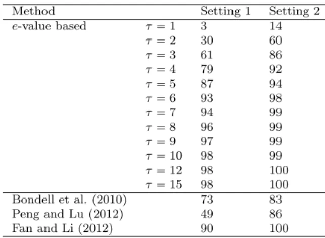
2.1 Comparison between our method and that proposed by Peng and Lu (2012) through average false positive percentage, false negative per-centage and model size . . . 48 2.2 Comparison of our method and three sparsity-based methods of mixed
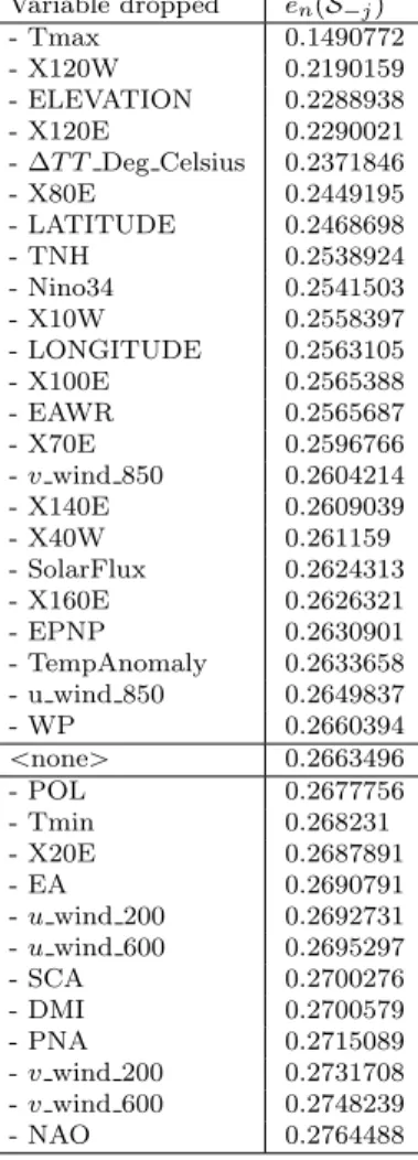
effect model selection through accuracy of selecting correct fixed effects 49 3.1 Ordered values of ˆenpSjqafter dropping thej-th variable from the full
model in the Indian summer precipitation data . . . 67 3.2 Average True Positive (TP) and True Negative (TN) proportions over
1000 replications for all three methods . . . 87 3.3 Average Relaxed True Positive (TPR) and Relaxed True Negative
(TNR) proportions over 1000 replications for all three methods . . . . 87 3.4 Table of analyzed genes and detected SNPs in them. Positive/ negative
sign indicates type of association found. . . 90 4.1 Table of AREpµw;µsqfor different spherical distributions . . . 103 4.2 Table of empirical powers of level-0.05 tests for the Chen and Qin (CQ),
WPL and Cn,w statistics . . . 105
4.3 Table of AREs of the ADCM for different choices of p and data-generating distributions, and two choices of depth functions . . . 119
4.4 Finite sample efficiencies of several scatter matrices: p 2, tv is t -distribution withv degrees of freedom, Np is p-variate normal . . . . 122
4.5 Finite sample efficiencies of several scatter matrices: p 2, tv is t -distribution withv degrees of freedom, Np is p-variate normal . . . . 123
4.6 Finite sample efficiencies of several scatter matrices: p 2, tv is t -distribution withv degrees of freedom, Np is p-variate normal . . . . 124
5.1 Average true positive and true negative (TP/TN) rates for 3 methods, for n50 and AR1 covariance structure . . . 160 5.2 Total runtimes in seconds for SGL and LARN algorithms for the three
simulation settings . . . 160 5.3 Top 10 gene-pathway connections inA. thaliana data found by LARN 162
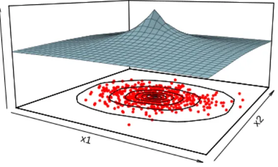
1.1 Depth is a scalar measure of how much inside a point is with respect to a data cloud: 500 points from N2pp0,0qT,diagp2,1qq . . . 2
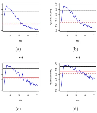
2.1 Empirical probabilities of selecting the correct model through moon bootstrap for several levels of sparsity: The e-values method- blue solid, AIC backward deletion- red dotted, AIC all subset- red solid, BIC backward deletion- black dotted, BIC all subset- black solid . . . 44 2.2 Empirical probabilities of selecting the correct model through gamma
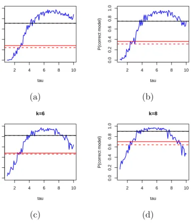
bootstrap for several levels of sparsity: The e-values method- blue solid, AIC backward deletion- red dotted, AIC all subset- red solid, BIC backward deletion- black dotted, BIC all subset- black solid . . . 45 2.3 Empirical probabilities of selecting the correct model through wild
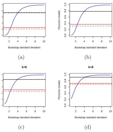
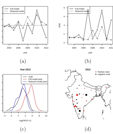
bootstrap for several levels of sparsity: The e-values method- blue solid, AIC backward deletion- red dotted, AIC all subset- red solid, BIC backward deletion- black dotted, BIC all subset- black solid . . . 46 3.1 Comparing full model rolling predictions with reduced models: (a)
Bias across years, (b) MSE across years, (c) density plots for 2012, (d) stationwise residuals for 2012 . . . 68
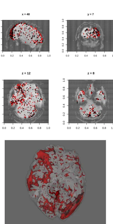
3.2 (Top) Plot of significant p-values at 95% confidence level at the spec-ified cross-sections; (bottom) a smoothed surface obtained from the
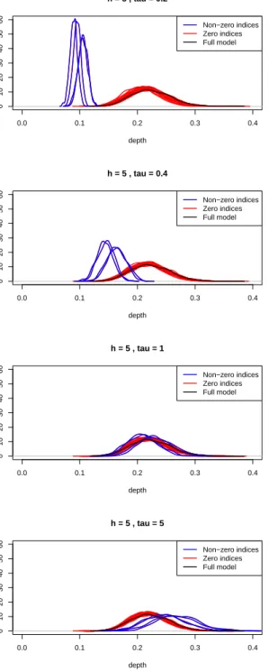
p-values clearly shows high spatial dependence in right optic nerve, auditory nerves, auditory cortex and left visual cortex areas . . . 73 3.3 Density plots for ˆDpτqand ˆDjpτqfor allj in simulation setup, with
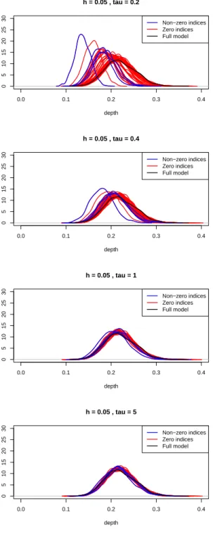
sig-nal parameter h5 and bootstrap standard deviationsτ 0.2,0.4,1,5 81 3.4 Density plots for ˆDpτq and ˆDjpτq for all j in simulation setup, with
signal parameter h 0.05 and bootstrap standard deviations τ
0.2,0.4,1,5 . . . 82 3.5 Plot ofe-values for genes analyzed: (a) GABRA2, (b) ADH1 to ADH7,
(c) SLC6A3 . . . 91 3.6 Plot of e-values for genes analyzed: (d) SLC6A4, (e) OPRM1, (f)
CYP2E1 . . . 92 3.7 Plot of e-values for genes analyzed: (g) DRD2, (h) ALDH2, (i) COMT 93 4.1 (Left) 1000 points randomly drawn from N2 p0,0qT,p5 44 5q
and (Right) their multivariate ranks based on halfspace depth . . . 107 4.2 Plot of the norm of influence function for first eigenvector of (a) sample
covariance matrix, (b) SCM, (c) Tyler’s scatter matrix and DCMs for (d) Halfspace depth, (e) Mahalanobis depth, (f) Projection depth for a bivariate normal distribution withµ0,Σdiagp2,1q . . . 116 4.3 Plot of the norm of influence function for first eigenvector of (a) sample
covariance matrix, (b) SCM, (c) Tyler’s scatter matrix and DCMs for (d) Halfspace depth, (e) Mahalanobis depth, (f) Projection depth for a bivariate normal distribution withµ0,Σdiagp2,1q . . . 126 4.4 Actual sample curves, their spline approximations and diagnostic plots
5.1 (a) Comparison of L1 and SCAD (Fan and Li, 2001) penalty functions with univariate halfspace depth: inverting the depth function helps ob-tain the nonconvex shape of the penalty function in the inverse depth; (b) Univariate thresholding rule for the LARN estimate assuming half-space depth and max definition of inverse depth(see Section 5.4) . . . 147 5.2 Mean squared testing errors for all three methods in different pp, qq
settings . . . 159 5.3 Estimated effects of different pathway genes on the activity of genes in
Mevalonate and Non-mevalonate pathways (left and right of vertical line) inA. thaliana . . . 161
Notation Meaning
E Expectation of a random variable (scalar/ vector/ matrix valued) V Variance of a scalar-valued random variable or covariance matrix of a
vector-valued random variable
P Probability of some event
Convergence in distribution
anbn anOpbnqand bnOpanq
}.} Euclidean norm for vectors, Frobenius norm for matrices, unless other-wise stated
an OPnpbnq an{bn converges to some c P R in probability conditional on the data
asn Ñ 8
anoPnpbnq an{bn converges to some 0 in probability conditional on the data as
nÑ 8 an
Pn
Ñbn an converges to bn in probability conditional on the data as n Ñ 8
Introduction
1.1
Background
The nonparametric concept of data depth had first been proposed by Tukey (1975) when he introduced the halfspace depth. The motivation behind this was to for-mulate a unified framework for nonparametric inference in multivariate concept: in particular, the multivariate equivalent of methods based on signs and ranks, order statistics, quantiles and outlyingness functions.
Given a dataset, the depth of a given point in the sample space measures how far inside the data cloud the point exists, i.e. it is a measure of centrality of the point with respect to the data. An overview of statistical depth functions can be found in Zuo and Serfling (2000). Depth-based methods have gained popularity in the past two decades, for robust nonparametric classification (Jornsten, 2004; Ghosh and Chaudhuri, 2005; Dutta and Ghosh, 2012; Sguera et al., 2014). In parametric estimation, depth-weighted means (Zuo et al., 2004) and covariance matrices (Zuo and Cui, 2005) provide high-breakdown point as well as efficient estimators, although they do involve choice of a suitable weight function and tuning parameters. As Liu and Singh (1997) have shown, it is also possible to use statistical depth functions in hypothesis testing and an alternate notion of p-values. Approaching data depth
x1 x2 Depth ● ● ● ● ● ● ● ●●● ● ● ●●●●● ●●● ●● ● ●●● ●●●●●● ●●●●● ●● ●●● ●●●●●●●●●●●●●●●●●●●●●●●●●●●●●●●●●●●●●●●●●●●●●●●●● ●●●●●●●●●● ●●●●●●●● ●●●●●●●●●●●●●●●●● ●● ● ●●●●●●●●●●●●●●●●●●● ●●●●●●●●●●●●●●●●● ●●●●●● ● ● ● ●●●●●●●●●●●●●● ● ●●●●●●●●●●●●●●●●●●●●●●●●●●●●●●●●●●●●●●●● ●●●●●●●●●●●●●●●●●●●●●●●●●●●●●●●●●●●●●●●●●●●●●●●●●●●●●●●●●●●●●●●●●●●●●●●●●●●●●●●●●●●●●●●●●●●●●●● ● ●●●●●●●●●●●●●●●●●●●●●●●●●●●●●●●●●●●●●●●●●●●●●●●●●●●●●●●●●●●●●●●●●●●●●●●●●●●●●●●●●●●●●●●●●●●●●●●●●●●●●●●●●●●●●●●●●●● ●●●●●●●●●●●●●●●●●●●●●●●●●●●●●●●●●●●●●●●●●●●●●●●●●●●●●●●● ●● ● ●
Figure 1.1: Depth is a scalar measure of how much inside a point is with respect to a data cloud: 500 points from N2pp0,0qT,diagp2,1qq
as from the perspective of breakdown points, Rousseeuw and Hubert (1999) also introduced the concept of regression depth, which was later generalized by Mizera (2002).
1.2
Definition and examples
For any multivariate distributionF taking values ˜Rp (or a subset of it), the depth of a pointxPRp, sayDpx, F
Xqis any real-valued function that provides a ‘center outward
ordering’ ofxwith respect toF (Zuo and Serfling, 2000). Figure 1.1 gives an intuition of data depth for samples from a bivariate normal distribution. As demonstrated by the contours and plot of values, a point close to the center, which coincides with the mean for elliptical distributions, has high depth. In other words, the point is situated deep inside the data/ underlying distribution. In comparison, a point closer to the periphery shall have less depth.
In order to standardizing this notion Liu (1990) outlined the desirable properties of a statistical depth function:
(P1) Affine invariance: DpAx b,AF bq Dpx, Fq for any A P Rpp,b P
Rp.
where XF;
(P2) Maximality at center: Dpθ, Fq supxPRpDpx, Fq for F having center of
sym-metry θ. This point is called the deepest point of the distribution.;
(P3)Decreasing from deepest point along any ray: Dpx;Fq ¤ Dpθ apxθq, Fq;
(P4)Vanishing at infinity: Dpx;Fq Ñ 0 as }x} Ñ 8.
In (P2) the types of symmetry considered can be central symmetry, angular sym-metry and halfspace symsym-metry. Also for multimodal probability distributions, i.e. distributions with multiple local maxima in their probability density functions, prop-erties (P2) and (P3) are actually restrictive towards the formulation of a reasonable depth function that captures the shape of the data cloud. Finally we think affine invariance is an artifact of depth functions being formulated keeping robustness with respect to elliptical distributions in mind, and in most practical cases a location and scale invariance suffices. Furthermore, because of their formulations, technical prop-erties like quasi-concavity, Lipschitz continuity, uniform convergence rise naturally in different definitions of data depth (Liu, 1990; Zuo and Serfling, 2000; Mosler, 2013).
It should be noted here that likelihood is not same as depth. Although in the univariate case many of these are essentially functions of the cumulative distribution function, and indeed for elliptical multivariate distributions depth contours coincide with density contours, unlike depths, likelihood is a local property. It is sensitive to multimodality, does not measure ‘inlyingness’ to a distribution in general and the maximum likelihood point may not be a central point according to any definition of symmetry (Serfling, 2006).
Some popular measures of data depth available in the literature and extensively used in nonparametric and semiparametric inference are as follows:
of all halfspaces containing a point. In our notations,
HDpx, Fq inf
uPRp;u0
PpuTX ¥uTxq
• Mahalanobis depth (MhD: Liu et al. (1999)) is based on the Mahalanobis distance of xto µ with respect to Σ: dΣpx,µq
a pxµqTΣ1pxµq. It is defined as M hDpX, Fq 1 1 d2 Σpx,µq
• Projection depth (PD: Zuo (2003)) is another depth function based on an outlyingness function. Here that function is
Opx, Fq sup
}u}1
|uTxmpuTXq|
spuTXq
where m and s are some univariate measures location and scale, respectively. Given this the depth atx is defined as P Dpx, Fq 1{p1 Opx, Fqq.
1.3
Why is depth not a thing yet?
Although some articles on data depth are fairly well-cited (e.g. Liu et al. (1999); Vardi and Zhang (2000)), in general it remains an esoteric, at best intriguing, con-cept in statistical literature. This is partly due to its nonparametric nature and high computational cost. There have been several approaches for calculating HD. A re-cent paper (Dyckerhoff and Mozharovskyi, 2016) provides a general algorithm that computes exact HD in Opnp1lognq time. PD is generally approximated by taking maximum over a number of random projections: and has high variability for small samples. MhD is easy to calculate since the sample mean and covariance matrix are generally used as estimates of µ and Σ, respectively. However this makes it less
robust with respect to outliers: defeating the purpose of using data depth in many situations.
A more significant reason though, we believe, is that the concept has not gener-alized enough since its first inception. There have been attempts at defining depth contours for distributions with nonstandard shapes (multimodal, star-shaped etc.) (Paindaveine and bever, 2013; Chernozhukov et al., 2017) as well as using functional depths (Narisetty and Nair, 2016; Sguera et al., 2016). These certainly broaden the domain of application for data depth. However, the scope of using depth, or depth-like quantities, is much larger in statistical inference. It quantifies the proximity of a point in a multivariate space to a probability distribution on the same space. In this spirit, given some hilbert spaceH, any such proximity measure D:HH˜ ÞÑ r0,8q,
˜
H being the space of probability measures on H, can be termed a depth function. Such quantities (or more accurately, decreasing transformations of them, e.g. the outlyingness function of Zuo and Serfling (2000)) provide a bridge between point norms and distributional distance measures like the Kullback-Leibler divergence or the Wasserstein metric in appropriate normed spaces. To the best of our knowledge, this generalized notion of point-to-distribution distance/ proximity is absent in the current literature. This thesis is an attempt in leveraging the extra flexibility provided by the above interpretation of data depth functions in diverse inferential scenarios.
1.4
Summary of work
In Chapter 2, we consider a general modelling framework in which several parameters need to be estimated from the data. Our objective here is to characterize subsets of the model space based on a pre-defined criterion, and to estimate this characterization in the presence of data. A concrete example for this can be variable selection in linear regression, where the user needs to find out the most parsimonious subset of
predictors that do not compromise the quality of model fit. For this purpose we introduce a function called the statistical evaluation map, which, while essentially serving the same purpose as depth, are based on much weaker assumptions and take into account the potentially expanding space of parameters. In a transformed space, this evaluates a function of estimated parameters corresponding to a specific subspace with respect to the sampling distribution of parameters from the full parameter space (i.e. the full model). The value of this evaluation function will change based on the specific sample the model estimates are based on, so this has a distribution as well, which depends on the sample size. We name the average evaluation function as the
e-value of a model: this acts as a quantification of model evidence. Under a very general definition of ‘good’ and ‘bad’ models we demonstrate how thesee-values can be used to differentiate between these two types. We use resampling to estimate the random distributions we work with: this is essential towards calculating sample version of model e-values. As a special case, when data depths are considered as evaluation maps, some further refinement can be achieved in the bifurcation of set of candidate models for the traditional statistical model selection problem. This results in an extremely fast, almost trivial, algorithm to separate out essential predictors in a regression-like setup.
Although depth functions did serve as our motivation for the above work and our initial results were assuming depths in elliptical sampling distributions of parameters, we later found out that a majority of the results hold in a much more generalized setup, and it is enough to explicitly invoke the usage of depths for variable selection only. As demonstrated in Chapter 3, the method ofe-values leads to valuable insights in several real data situations. In Section 3.3 therein, we expand the scope ofe-values by considering tail quantiles of evaluation map distributions as e-values instead of their means: this leads to improved detection of weak single nucleotide polymorphism signals in behavioral trait analysis of genetic data from families.
Chapter 4 onwards we take a more mainstream approach. Here we introduce a composition of the spatial sign function (Locantore et al., 1999) with transformations on functions that are essentially the outlyingness maps of Zuo and Serfling (2000), with a few restrictions for technical convenience. After a brief consideration of its per-formance in the location problem for elliptical distributions, we define a multivariate rank vector using this. We discuss several aspects of its performance in estimating components of the covariance matrix in the data-generating elliptical distribution: its eigenvectors, eigenvalues and the covariance matrix itself. Several simulation studies and data examples outline the utility of these methods, and we also discuss their implementation in Sufficient Dimension Reduction (Adragni and Cook, 2009) and functional outlier detection.
Chapter 5 discusses another application of the idea of data depth-based inverse ranking, this time in regularized regression. We propose a new class of noncon-vex penalty functions in the paradigm of multitask sparse penalized regression using penalties based on data depth. Focusing on a one-step sparse estimator of the co-efficient matrix using local linear approximation of the penalty function, we derive its theoretical properties and provide the algorithm for its computation. For or-thogonal design and independent responses, the resulting thresholding rule enjoys near-minimax optimal risk performance, similar to the adaptive lasso (Zou, 2006). A simulation study as well as real data analysis demonstrate its effectiveness com-pared to some of the present methods that provide sparse solutions in multivariate regression.
Generalized Model Discovery using
Statistical Evaluation Maps
2.1
Introduction
In a typical statistical or data science exercise, both data and astatistical model are involved. While there is often little or no ambiguity about data, there can be many alternatives about how to analyze such data, and how to interpret the results. This broadly constitute the realm of statistical models. In this chapter, we interpret the term statistical model very broadly. We recognize that various possible transforma-tions of the data, different model fitting algorithms, practical safeguards put in place to ensure robustness and sensitivity balance in the results, different methods of data analysis, different statistical paradigms of interpretation of results, as all equally de-serving to be considered as crucial components of a statistical model. The example below illustrates this idea.
Example 2.1.1 (Tree data). Consider the data contained indata(trees)in the sta-tistical softwareR. There are 31 observations on girth, height and volume. Observed data for these variables arepX1i, X2i, Yiq respectively, for for i1, . . . , n. We denote p2 for the two explanatory variables X1 and X2, used to explain the properties of
the response variable Y.
Define the Box-Cox transformation (Box and Cox, 1964) on the response variable as Cpy, λq logpyqIλ0 yλIλ0. We assume that Yi’s in the data are related to the
other variables according to the statistical relation
CpYi, λq β0 βlogpX1iq βlogpX2iq ei (2.1.1)
Here teiuis a sequence of random variables, and we assume that Eei 0 and Ee2i σ2
i 8. The parameters in this system are θn pλ, β0, β1, β2, σ12, . . . , σnq P2 Rpn
where pnn 4.
Even in this rather simple framework, we can imagine several statistical models
as being per se equally interesting or important. These can include (i) the Gauss-Markov linear regression model withλ 0, (ii) linear regression with any other fixed, non-randomλ, (iii) a model whereλ is estimated form data but then a linear regres-sion model used for the rest of the analysis ignoring the randomness in the estimated
λ, (iv) using a fixed λ value like 0 or 1, then using ordinary least squares (OLS) method to estimate regression parameters, followed by inference based on the resid-ual bootstrap (see Efron (1979); Efron and Tibshirani (1993); Shao and Tu (1995)), (v) using robustness-driven M-estimation techniques for simultaneous estimation of
pλ, β0, β1, β2q, followed by awild bootstrap resampling scheme for statistical inference
(Wu, 1986; Mammen, 1993), which provides robustness against heteroscedasticity. We submit that these are all plausible models, important from one or more con-siderations. Some like (iii) reflect tradition, others like (v) reflect desirable caution coupled with modern computational power. The above list of possible models is far from exhaustive (e.g. in (iv) each alternative resampling scheme may be called a separate model), but serves to illustrate the fact that statistical models arise in most of the standard procedures of data analysis, be it from classical Statistics, robustness considerations, Bayesian paradigm, risk management perspective, Occam’s razor, or
combinations thereof. Such models typically differ from each other in many ways, and not just in the number of covariates, or number of parameters to estimate. Often, as in the case of the heteroscedastic model coupled with resampling-based inference above, a very classical approach towards modeling or model selection, or a selection based only on a superficial reading of parsimony, can lead to leaving out greatly versa-tile models on both robustness and efficiency counts. In this chapter, we address this problem of elicitation of suitable models for analyzing data in a very general frame-work. We consider candidate models that need not be nested, or philosophically or otherwise compatible with each other.
Our primary goal is a clear separation of the candidate models into two groups: those that adequately explain some user-defined characteristics exhibited in the data, which we designate adequate models, and those that do not (inadequate models). The first subsection in Section 2.2 contains notations and a technical definition of model adequacy, as well as a generic description of a baseline model, which we call the preferred model. This may be the most complex candidate model (e.g. the model with all covariates in regression), a model in popular or current use, a hypothesized model, or a model with known parsimony or computational advantage. As we shall see, this formulation of statistical models is broader than the traditional definition of correct or wrong models in model selection literature (e.g. Shao (1993, 1996)). Each candidate model has its own set of unknown parameters, which are estimated using a model-specific optimization framework. The next subsection outlines this estimation method. Following this, all model parameter estimates are mapped to a common Euclidean reference frame Rdn, d
nPN through user-defined transformation functions
for ease of comparison between models.
We focus on this transformed model spaceRdn, and propose using a function called
the evaluation map in Section 2.3, which compares each candidate model against the preferred model. An evaluation map typically compares a point in the parameter
space of any candidate model with the distribution of estimated parameters in the preferred model, and data depth functions are special cases of functions that may act as an evaluation map. After this we introduce a quantity called the e-value, which we define as a non-negative summary statistic for the evaluation map distribution corresponding to a candidate model. The model e-value is a measure of how well a candidate model explains the interesting features of the data, which is based on a user-specified function. Under very general theoretical conditions we show that population
e-values for theoretical models asymptotically tends to zero, while for adequate models they tend to the e-value of the preferred model. Thus we allow the possibility that none of the candidate models, including the preferred model, adequately explain the properties of the data at hand. In such cases, only the preferred model will have a high score. Our proposal thus includes the provision for triggering a re-evaluation of models and data based on scientific caution, when only the preferred model achieves a significantly non-zero score.
We adopt a fairly general resampling-based procedure to approximate the dis-tribution of evaluation maps for a candidate model, and in Section 2.4 establish consistency of the resampling procedure adopted in this chapter, when one or more models are considered simultaneously. Following this we show that under certain conditions on the resampling schemes, population e-values for both adequate and in-adequate models can be consistently recovered. Thus, we formulate a unified system where resampling elicits both the e-value of a model, along with the joint sampling distribution of all its parameter estimators. This allows for automatic inference and prediction with any model.
Additionally, in Section 2.3 and Section 2.4 we allow several quantities, like num-ber of parameters in each candidate model or the numnum-ber of characteristics of interest from the data on which the evaluation map is computed, to tend to infinity with sam-ple size. This dimension asymptotics approach allows any candidate model to have
increasing parameter dimensionality with sample size, which imitates the reality of the scientific discovery process where additional data is often used in conjunction with more fine-tuned or insightful models. Similarly, allowing the number of characteristics used for comparing models to grow with the sample size reflects the scientific process. Throughout these sections, for theoretical purposes we adopt a framework involving a triangular array of models and parameters, where various parameter values and di-mensions and even estimation and model evaluation procedures are allowed to change with sample size. This is partially for the same reason of being in tune with the real-ity of scientific discovery process, but also for additional theoretical advantages that such a framework offers, and for the purpose of being inclusive of techniques like local asymptotics, uniform convergence and several others that will form part of our future work.
Our proposal thus far involves four choices: that of (a) a preferred model, (b) a map from the parameter space to Rdn for each candidate model, (c) an evaluation
map, which is a function defined on Rdn and probability distributions on it to
com-pare each model to the preferred model, (d) a resampling strategy. In Section 2.5 we demonstrate how all of these come together in tackling the traditional model selection problem of identifying necessary covariates in a regression-like setup. In such prob-lems, there is a maximum number of parameterspnto consider, and various candidate models consider subsets of a common set ofpnparameters. The candidate models can
be arranged in a lattice, with the supremum being theleast parsimonious or complete model that involves all pn parameters. There are 2pn such models, and a full
evalu-ation of all such models is an NP-Hard problem (Natarajan, 1995). For this reason various algorithms to reduce computations by evaluating far fewer models (Schwarz, 1978; Konishi and Kitagawa, 1996), as well as sparsity-based approaches (Tibshirani, 1996; Fan and Li, 2001; Zou, 2006) have been proposed, which compromise optimality and other properties of the model selection procedure.
In this context, we use data depths as evaluation functions, allowing us to estab-lish a preference ordering among the adequate models. Subsequently we are able to propose a very fast algorithm which has the following simple and generic steps:
1. Start from the model with all covariates, i.e. the full model and compute its
e-value using resampling;
2. Take the marginal models by dropping each covariate, compute their corre-sponding e-values;
3. Collect covariates that cause a decrease in e-value compared to the full model. As evident from the above steps, this recipe only requires computation of the full model. Coupled with the fact that a fast and parallelizable generalized bootstrap procedure (Chatterjee and Bose, 2005) based on Monte-Carlo simulation can be used as the resampling method of choice, we end up with an extremely fast covariate se-lection method. This procedure is able to tackle with ease tricky modelling situations like linear mixed models and robust regression, and also provides asymptotic model selection consistency owing to the machinery developed in Section 2.3 and Section 2.4. In Section 2.6 we present two illustrative examples on how our fast algorithm is implemented, and its relative performance in covariate selection problems. One of the examples in this section involves random effects, to illustrate the breadth of applicability of the proposed methodology. Finally, in Section 2.7 we discuss the scope and implications of this framework, future research plans, caveats and end with some concluding comments. Regarding real data applications of thee-values procedure, we have performed substantial amounts of them in diverse modelling situations: this we are going to defer to Chapter 3.
function h of the parameters in any model, we will often simplify notations by using hhsnhpθsnq, p h phsnh p θsn , p hr phrsnh p θrsn .
The notation an bn implies that an Opbnq as well as bn Opanq. The notation
R, typically with various subscripts like Rn,Rsn,Rrsn and so, are used as generic
for remainder terms, which contribute asymptotically negligible terms in our results. While we include all necessary algebraic details, often the tedious algebra behind moment calculations and probabilistic bound computations is omitted to contain this chapter to a reasonable length and preserve clarity. However, our technical conditions are always comprehensive and explicit, and such algebraic computations can be easily carried out without much intellectual effort. In designing the technical conditions for the theoretical properties in this chapter, we have striven for simplicity and not on minimal requirements. Thus, the various assumptions made in this chapter are often sufficient conditions, rather than necessary ones, for the theoretical results.
2.2
The general framework
2.2.1
The frame of models
In any statistical model, each parameter has an assigned role. A parameter may be a constant related to the scientific process, tuning constant related to a computational procedure or a prediction algorithm, or may perform some other function. Examples of the former in Example 2.1.1 are the regression slope parameters β1 and β2, which
exam-ple of the latter in the same context can be the parameterλ, or a tolerance or iteration limits of an iterative model fitting procedure. Parameters can have similar roles in many models, for example, the regression coefficients β1 and β2 in Example 2.1.1 are
used in all the listed models in that example. We use these general facts to describe
frame of models that we use in this paper.
In this chapter, we consider a context where the union of all parameters from all candidate models forms a countable set. Naturally, problems where the number of parameters are finite, as in a majority of statistical applications, are included in our framework. We exclude all constants that are invariant across candidate models from this count, or any unknown quantity that is not estimated in any model and is not used subsequently. The parameters across all models are laid out in any arbitrary but fixed fashion indexed by the set of integers t1,2, . . .u. For example, in 2.1.1 we may consider pnn 4 as the maximum number of parameters in the system, and denote the pn-dimensional vector of parameters with the generic notation
θn λ, β0, β1, β2, σ12, . . . , σ 2 n θn,1, θn,2, . . . , θn,pn notationally.
We now associate a candidate modelMn, either from a scientific discovery process
or a hypothesis testing process, with two quantities:
(a) The set Sn tj1, . . . , jpsnu t1,2, . . .uof indices where the parameter values are
unknown and estimated from the data; and
(b) An ordered vector of known constants cn pcnj : j R Snq for parameters not
indexed by Sn.
For any n the sets Sn are finite, thus each model may include only a finite number of
unknown real-valued constants.
Θn
jΘn,j, will thus have the structure
θmnj $ & % Unknown θmnj for j PSn; Known cnj for j RSn.
Each θmnj R, thus all parameters are real-valued. It may be noted that in most
cases, simple re-parametrization can be used to define models in a way such that the known constants in cn are all zero.
We assume that at stage n there is have a preferred model, which we denote by
Mn: and is identified by the set of indices Sn t1,2, . . .uhavingpn elements, and
known constants cn. We also designate a a fixed element of Mn as the preferred
parameter vector, sayθ0n. Depending on the context, the preferred model may relate
to a hypothesized model, or the most complex or the most simple model, or relate to the current state of the art, a ‘gold standard’, or be ‘preferred’ by some other predefined criteria; whereas the preferred parameter vector is generally indicative of the data generating process. Note that the preferred model is just one of the candidate models, and its usage will shortly be clear.
2.2.2
Transformation to a common platform
Suppose Gmn :ΘnÑRdn is a known transformation to map parameters from model
Mn to Rdn. While the candidate models may be very diverse and may relate to
different physical realities, theories or hypotheses, computational or data analytic choices, the Euclidean spaceRdn is a common ground where all models may be
com-pared. We use the notation Gn for the transformation of the preferred model. In
principle, each Gmn can also be designed to map to some proper subset Gn of Rdn.
However, in such cases we would have to address technical issues relating to topo-logical, measure-theoretic and geometric or algebraic properties of Gn while studying
theoretical results, which may be considered avoidable since the statistician gets to choose the maps Gmn. Consequently, we assume that the co-domain of each map
Gmn is Rdn in this paper, and avoid unnecessary mathematical complications.
The choice of Gmn may depend on the purpose for building the scientific model,
and the way we interpret the model. This transformation allows us to consider the
science case where the actual parameter values and their interpretation is subject to scrutiny, or use cases like prediction and classification problems.
Example 2.2.1 (Example 2.1.1 continued). In Example 2.1.1 consider the three types of models:
1. Linear regression model: Yi Xi1β1 Xi2β2 i, i Np0, σ2q with σ ¡0 for i1, . . . , n;
2. Semiparametric regression model: Yi Xi1β1 gpXi2q i, for an unknown
function g;
3. Semiparametric single index model: Yi hpXi1β1 Xi2β2q ifor some unknown
function h.
If we consider only the linear regression model and are interested in the estimated linear effects on the covariates, any candidate model Mn shall correspond to Sn t1,2u and cn P R2|Sn|. Consequently an identity transformation for all models is
enough to put them in a comparable platform. However, when all three types of models above are considered together, comparing and choosing between them becomes tricky. While it is certainly possible consider all modelling methods as special cases of a general model: Yi hpXi1β1 gpXi2qq i in presence of suitable technical
conditions, restrict hp.q in (3) and gp.q in (2) as linear combinations of elements in some B-spline basis, and represent a model as a collection of elements in the space of the combined set of spline basis coefficients: it makes their interpretation less
intuitive. A more interpretable platform in this scenario can be the predicted value of responses, and one can simply take asGmn the vector of fitted values obtained in
each method.
We now define an important concept for use in the rest of this paper. Each candidate model corresponds to a subspace of the full parameter space Θn. For any
given modelMn, entries of its corresponding subspaceΘmn are specified by elements
fromΘj for indices j PSn, and entries fromcnwhen j RSn. Consequently, we define
their versions in the transformed space Gn:
Gmn : tGmnpθpMnqq:θpMnq PΘmnu
Gn : tGnpθpMnqq:θpMnq PΘnu
In this framework,
Definition 2.2.2. Forg PRdn and G1
n Rdn, we define the following:
dpg,Gnq1 : inf
g1PGn1
}gg1}
where }.} is the Euclidean norm. Then
(a) For two sequences of models, say tM1nu and tM2nu, we say tM1nu is nested
within tM2nu if, for all sequences tg1n :g1nP G1nu we have
lim
nÑ8dpg1n,G2nq 0 (2.2.1)
(b) A sequence of models tMnu is called adequate if the model M0n corresponding
to the singleton set Θ0n tθ0nu, i.e. when S0n H and c0n θ0n, is nested within
Mn.
This notion of adequacy of a model depends on the choice of the preferred param-eter vector, as well as the transformation maps Gmn. The preferred model is always
adequate, as is M0n, so the set of adequate models is non-empty by construction.
Since the notion of parsimony is important in this context, we define the minimal adequate model as the adequate model that has the smallest number of parameters estimated from the data. Our framework ensures that there is always a minimal adequate model (M0n), though in general, its uniqueness is not guaranteed.
In classical model selection problems, as in linear regression where a subset of covariates Xs is used in fitting the expression Y Xsβs , this concept of model
adequacy captures standard notions of model ‘correctness’. Given a full-rank covariate matrix X P Rknp, candidate models are fully specified by the set S P t1, . . . , pu of
non-zero indices in β, and for obvious choices of tGmnu, the condition for model adequacy reduces to EY Xsβs 0. Thus the concept of the minimal adequate
model merges with that of a ‘true model’ used in many studies.
We elicit the above broader definition to capture the limiting cases that arise in such situations. For instance, in the above example considerp2 and the triangular data generating model to be Yni X1iβ01 X2iδn for some β01 P R, δn op1q
and i 1, . . . , kn. In our framework, given that the model with all covariates is the
preferred model, the sequence of models Mn so that Θmn tpβ1,0qT :β1 PRu shall
be considered an adequate model. Such models frequently arise from prior choices in bayesian variable selection techniques (e.g. Narisetty and He (2014); Ro˘ckov`a and George (2016)).
2.2.3
Method of estimation
Since some or all the parameter values are unknown in a typical scientific problem, they have to be estimated from empirical observations. Suppose at stage n, the empirical data we have at hand is denoted by the setBn tBn1, . . . , Bnknu, where we
do not restrict either the dimension of any of the Ani’s, or declare any properties or restrictions on them. In particular, eachBni may be infinite dimensional element, or
a finite dimensional vector. The size of Bn, which we call thesample sizeand denote
bykn is assumed to be a non-decreasing sequence of integers that tends to infinity as nÑ 8.
We consider here a known triangular array of functions, say Ψmnipq, for which the following equation has a unique minimizer in Θmn:
Ψmnpθq E kn ¸ i1 Ψmni θ, Bni (2.2.2)
for any candidate model Mn. Suppose this minimizer is θmn. We borrow the
termi-nology energy function from optimization and other literature to denote such func-tions. They functions have also been called contrast functions, (see Pfanzagl (1969); Michel and Pfanzagl (1971); Bose and Chatterjee (2003)). The estimator ˆθmn of θmn
is obtained as a minimizer of the sample analog of the above, i.e.
ˆ θmnarg min θPΘmn kn ¸ i1 Ψmni θ, Bni (2.2.3)
The preferred model estimate, say ˆθn is described in an identical way. Thus
ˆ θnarg min θPΘn kn ¸ i1 Ψni θ, Bni (2.2.4)
where Ψnipq are a known triangular array of functions.
Naturally, only the unknown elements of the generic model vector θ, say θpSnq, and their sample equivalents are relevant for the above minimization problems. Hence for ease of exposition we shall assume that Ψmnipθ, .q ΨsnipθpSnq, .qfori1, . . . , kn,
estimated.
We designate the subvector of θmn at indicesSn byθsn, and assume the following
very general conditions on this estimation process:
(S0) For inadequate models, the model corresponding to the singleton set tθmnu
Θn is inadequate.
(S1) Define the Hilbert space `2 ttxn, n 1,2, . . .u : xn P R, °
n¥1x
2
n 8u,
and embed Rpsn in it as and when necessary, as the first p
sn |Sn| elements of `2.
Denote by rθs the probability distribution of the random variable θ. Then for any candidate model Mn there exists a tight sequence of probability measures Tsn on `2
with weak limitTs,8 P`˜2, which is the set of probability measures on`2, and positive
real numbers asnan such that
(a) For all n,
asn
ˆ
θsnθsn is the distribution of the marginal of Tsn under the
first psn coordinates;
(b) For the preferred model solution θn, }anpGnG0nq} Ñ0 as n Ñ 8.
Because of the definition of inadequate models, we need (S0) to ensure that the sequence of solutions for inadequate models do not actually end up converging to the preferred model vectorθ0n. We need (S1) to prove the population-level results in the
next section, covering potentially biased estimation methods with bias going to 0 as
n grows. A few technical conditions will eventually get added to this in Section 2.4 to establish consistency results of the resampling scheme used.
2.3
Statistical evaluation maps and
e
-values
2.3.1
A general evaluation map
We now introduce another function, the statistical evaluation function:
En:RdnR˜dn Ñ r0,8q
which takes as arguments a point from Rdn and a probability measure from ˜
Rdn, and
maps that pair into a non-negative real number. Roughly, the quantity Enpy,rYsq
is a measure of where exactly the point y sits with respect to the distribution of the random variable Y PRdn.
The exact nature of the evaluation function, which will make this rough notion precise, depends on the context. We shall discuss this in detail shortly. Good examples of evaluation functions are probabilities of sets likeAδ tx:|x| δu underNp0, σ2q
distribution forσ ¡0, unimodal probability density functions that uniformly decrease away from the mode in any direction, and various data depth functions. In fact, depths offer a very rich collection of relevant functions: although their properties are somewhat more restrictive than those our evaluation map requires initially. While we later use halfspace depth (Tukey, 1975) as our choice of evaluation map in model selection, for the majority of our theoretical analysis we do not restrict the evaluation maps to be only depth functions in order to avoid some of technical assumptions on traditional depth functions that are not required in our context until Section 2.5.
2.3.2
The
e
-value of models
We now associate with each modelMna functional of the evaluation map En: which
we call the e-value. An example of e-value is the mean evaluation map function:
enpMnq EEn
ˆ
Gmn,rGˆns (2.3.1)
which we concentrate on for the rest of the paper. However, any other functional of EnpGˆmn,rGˆnsq may also be used here, and a large proportion of our theoretical
discussion in the rest of the paper is applicable to any smooth functional of the distri-bution of EnpGˆmn,rGˆnsq. Furthermore, the distribution of EnpGˆmn,rGˆnsq is itself informative, and has an important role to play in the study of uniform convergence. We defer all this discussion and analysis to future research.
Remark. From a hypothesis testing perespective, e-values generalize the concept ofp-values. Consider the problem of finding out the right tail probability with respect to a null distribution, say rT0ns, for a test statistic ˆTmn. Here we can designate the
model corresponding to the null hypothesis as the preferred model, take the smooth transformation as Gmn Tmnˆ and given the evaluation map EnpTn,ˆ rT0nsq ITˆn¡T0n
the e-value is calculated as PpTˆn ¡ T0nq. A higher e-value (or p-value) indicates a
high degree of similarity between the null and alternate model, or in other words the alternate model is ‘adequate’ for the null model. However, in terms of usefulness the inadequate models will be the useful ones in this context.
There are two random quantities involved in the expression of epMnq above, namely ˆGmnand ˆGn. Typically, the distribution of either of these random quantities
are not known, and have to be elicited from data. We shall use resampling methods for this purpose, the details of which will be outlined in later sections.
2.3.3
Model adequacy and
e
-values
We now present our first result on the model elicitation process, which as claimed earlier, separates the inadequate models from the adequate ones.
For this, we first assume two conditions on the transformation Gmn. Note that
the j-th element of the function Gmn, denoted by Gmnjpq Gjpq, is a map from a
subset of Rpn to
R, forj 1, . . . , dn. Here we assume that
(G1)dnopminSntasn, anuq;
(G2) The functions Gjpq are smooth functions in a neighborhood of θmn θ.
Specifically, there exists a δ ¡ 0 such that for x θ t with }t} δ, we have the following expansion
Gjpxq Gjpθq GT1jpθqt 2 1
tTRjpθ ctqt (2.3.2)
for some cP p0,1q. We assume that there is a positive definite matrix Mj such that
sup
t:}t} δ
Rjpθ ctq Mj; λmaxpMjq 8 (2.3.3)
Also, the technical conditions assumed on the sequence of evaluation maps are as follows:
(E1) Each En is invariant to location and scale transformations, i.e. for any a P
R,bPRdn and random variableG having distribution GP R˜dn,
Enpx,Gq Enpax b,raG bsq (2.3.4)
αn ¡0, possibly depending on the measure GPG˜n such that
|Enpx,Gq Enpy,Gq| }xy}αn (2.3.5)
(E3)SupposetYnuis a tight sequence of probability measures on`2, with weak limit
Y8. Further assume that Yn P Rdn is a random variable that follows the marginal
distribution of the first dnco-ordinates under Yn. Also supposeE8 :`2`˜2 Ñ r0,8q
be a map such thatEE8py,Y8q 8, and when restricted to the firstdnco-ordinates, E8 matches En. Then we assume that
lim
nÑ8EEnpYn,rYnsq EE8py,Y8q (2.3.6)
(E4) Now suppose that Zn PRdn is another sequence of random variables. Then, if }Zn}Ñ 8P , we assume the following condition as nÑ 8:
EnpZn,rYnsq P
Ñ0 (2.3.7)
Clearly, these properties are not mutually exclusive, and some may be derived from others, but we present these together for ease of verification. Additionally some properties like Lipschitz continuity and (E4) are simply for technical convenience, while we only require the condition (E3) that is weaker than uniform convergence.
We are now at a stage to present our population-level result that forms the foun-dation of all the following analysis.
Theorem 2.3.1. Consider a sequence of evaluation functionsEnsatisfying properties
(E1)-(E4). Then as n Ñ 8:
1. For the preferred model Mn, enpMnq Ñe8 8;
3. When Mn is an inadequate model, enpMnq Ñ0.
This result ensures that for large enough n, it is possible to find some threshold
n ¤enpMnqsuch that all inadequate models have e-values less than the threshold, while e-values for all adequate models fall above it. The choice of n, of course,
depends on several factors like the evaluation map, estimation technique used and sample size: some cases of which we shall pursue later (Section 2.5 and Section 3.3).
2.4
Estimation of
e
-values through resampling
In this section we shall use a resampling scheme to estimate the distributions corre-sponding to the smooth functionals of candidate model parameters we consider, i.e.
ˆ
Gmn, and discuss consistency of the resulting procedure in estimating modele-values
through imposing certain necessary conditions on the resampling scheme used. A special case of the family of resampling methods that we use in this chapter is the m-out-of-n bootstrap, which we abbreviate as moon bootstrap. There are nu-merous problems where the moon-bootstrap provides consistent approximation to the distribution of statistics of interest (e.g. Shao (1996); Chatterjee and Bose (2005)). Since all such cases are too numerous to list and review of resampling consistency is not central to this chapter, we only demonstrate the properties of our resampling procedure in some interesting frameworks.
Recall that in (2.2.3) and (2.2.4) we obtain the estimator ˆθmn by minimizing
the energy functional or estimating functional Ψˆsnpθq °kn
i1Ψsnipθ, Bniq. The
parameter θmn is the unique minimizer of the expectation of the above over all θ P
Θmn. In this section, we occasionally drop the subscriptsandwhen there is no scope
for confusion for notational simplicity, since the developments presented in the rest of this section are applicable to any model. We often drop the second argument from estimating functionals, thus for example Ψnipθq Ψsnipθ, Bniq. Any other notational
simplifications in various contexts of this section will be presented as related contexts arise.
2.4.1
Smooth estimating functional models
We shall consider the case is where the functions Ψsnip,q is smooth in the first
argument, which covers a vast number of models routinely considered in statistics. In a neighborhood of θsn, which is the solution of Ψsn
°
iΨsni, we assume that
the functions Ψsni are thrice continuously differentiable in the first argument, with
the successive derivatives being denoted by Ψksni, k 0,1,2. That is, there exists a δ¡0 such that for any θ θsn t satisfying }t} δ we have
d
dθΨsnipθq Ψ0snipθq PR
psn (2.4.1)
wherepsn |Sn|. For theathelement of Ψ0snipθq, a1, . . . psn, denoted by Ψ0snipaqpθq,
we have
Ψ0snipaqpθq Ψ0snipaqpθsnq Ψ1snipaqpθsnqt 21tTΨ2snipaqpθsn ctqt (2.4.2)
for some cP p0,1qpossibly depending on a. We assume that for eachSn andn, there
is a sequence of σ-fields Fsn1 Fsn2. . .Fsnkn such that t
°j
i1Ψ0snipθsnq,Fsnju is a
martingale.
Also, let the spectral decomposition of the matrixΓ0sn °kn
i1EΨ0snipθsnqΨT0snipθsnq
be given by
Γ0sn P0snΛ0snPT0sn (2.4.3)
where P0sn P RpsnRpsn is an orthogonal matrix whose columns contain the
that Γ0sn is positive definite, that is, all the diagonal entries of Λ0sn are positive
numbers. We assume that there is a constant δ0s¡0 such that λminpΓ0snq ¡δ0sn for
all sufficiently large n. The matrices Λc0sn for various real numbers c are defined in the obvious way, that is, these are diagonal matrices where the j-th diagonal entry is raised to the power c.
LetΓ1snipθsnqbe thepsnpsnmatrix whosea-th row isEΨ1snipaqpθsnq; we assume
this expectation exists. Define
Γ1snpθsnq
kn
¸
i1
Γ1snipθsnq (2.4.4)
We assume that Γ1sn Γ1snpθsnq is nonsingular for each Mn and n. Suppose the
singular value decomposition ofΓ1sn is given by
Γ1sn P1snΛ1snQT1sn (2.4.5)
whereP1sn,Q1snP RpsnRpsn are orthogonal matrices, andΛ1snis a diagonal matrix.
We assume that the diagonal entries ofΛ1snare all positive, which implies that in the
parameter space the energy functional Ψsn actually achieves a minimal value atθsn,
the solution of the optimization problem. We define the matrices Λc1sn for various real numbers c as diagonal matrices where the j-th diagonal entry is raised to the power c. Correspondingly, we define Γc1sn P1snΛc1snQT1sn, and assume that there is
a constantδ1sn¡0 such that λminpΓ1TsnΓ1snq ¡ δ1sn for all sufficiently large n.
We now define the matrix
Asn:Γ
1{2
0sn Γ1sn. (2.4.6)
(S2) The minimum eigenvalue of ATsnAsn tends to infinity. Specifically, for the
se-quence asn Ò 8 from condition (S1), we have
λmin Γ1snΓ0sn1Γ T
1sn
a2sn (2.4.7)
(S3) Also there exists a sequenceτsnÒ 8, τsn1 Op1q asn Ñ 8such that λmax Γ1sn1Γ 2 0snΓ 1T 1sn opτsn2q (2.4.8)
as nÑ 8 for any Sn, and
E Asn1 k n ¸ i1 Ψ1sniΓ1sn Asn1 2 F oppsnτsn2q (2.4.9)
where }A}F denotes the Frobenium norm of matrix A.
(S4) For the symmetric matrix Ψ2snipaqpθq and for some δ0 ¡ 0, there exists a
sym-metric matrix M2snipaq such that
sup }θθmn| δ0 Ψ2snipaqpθq M2snipaq, (2.4.10) satisfying psn ¸ a1 kn ¸ i1 Eλ2max M2snipaq o a6snn1psnτsn2 (2.4.11)
For any vector cP Rpsn with }c} 1, define Z
mni cTΓ 1{2 0sn Ψ0sni for i 1, . . . kn. We assume that kn ¸ i1 Z2sniÑP 1, and E max i |Zsni| Ñ0. (2.4.12)
from hereon using ΨksniΨksnipθsnq, fork 0,1,2.
We now consider an array of resampling weights Wrsni, which for any n may be
collected together in the vector Wrsn pWrsn1, . . . ,Wrsnknq
T P
Rkn. We assume
that this is an exchangeable array of non-negative random variables, independent of the data. The index r denotes that these are related to the resampling procedure. The actual implementation of the resampling procedure is carried out by generating independent copiestW1sn, . . . ,WRsnufor some sufficiently large integerR, and using
them in a Monte Carlo procedure, where for anyr 1, . . . , R, we minimize
kn
¸
i1
WrsniΨmnipθ, Bniq (2.4.13)
to obtain the resampling version of the estimator ˆθrsnPRpsn. This is the generalized
bootstrap (Chatterjee and Bose, 2005).
We assume that for each i1, . . . , kn,EWrsni µsnandVWrsni τsn2 , and write
the centered and scaled resampling weights as
Wrsni τsn1pWrsniµsnq, (2.4.14)
thusWrsniµsn τsnWrsni. Since Wrsni ¥0 almost surely and is non-degenerate, we
haveµsn¡0, and assume that µsn τsn2 Opτsnq2 . Our analysis below suggests that
the properties of the resampling procedure depend only on thecoefficient of variation
We assume the following conditions on the resampling weights as n Ñ 8: EWrsn1 µsn, (2.4.15) VWrsn1 τsn2 Ò 8, (2.4.16) τsn2 opa2 snq, (2.4.17) EWrsn1Wrsn2 Opkn1q, (2.4.18) EWrsn2 1W 2 rsn2 Ñ1, (2.4.19) EWrsn4 1 8. (2.4.20)
Example 2.4.1 (The m-out-of-n (moon) bootstrap). In our framework, the moon -bootstrap is identified with Wrsn having a Multinomial distribution with
parame-ters m and probabilities k1
n p1, . . . ,1q P Rkn, by a factor of kn{m. Thus we have
EWrsn1 µsn pm1knqpm{knq 1, and VWrsn1 τsn2 pm1knq2pmkn1p1 k1
n q Opm1knq. In typical applications of the moon-bootstrap, as in its
applica-tion in this chapter, we require that m Ñ 8 and m{kn Ñ 0 as n Ñ 8. Thus we
have τ2
sn Ñ 8 as n Ñ 8, thus the scale factor of the resampling weights Wrsni tend
to infinity with n. We use the term scale-enhanced resampling for schemes like the
moon-bootstrap where the variance of (properly centered) resampling weights tends to infinity with n.
Example 2.4.2 (The scale-enhanced Bayesian bootstrap). A version of Bayesian bootstrap may be constructed by choosing Wrsni to be independent and identically
distributed Gamma random variables, with mean µsn 1 and variance τsn2 Ñ 8 as nÑ 8. The functionality of this resampling scheme and Bayesian interpretation re-main similar to the standard Bayesian bootstrap, however some convenient properties like conjugacy are lost.
Theorem 2.4.3. Assume conditions (S0)-(S5) and thatp2
Addi-tionally, assume that the resampling weightsWrsni are exchangeable random variables
satisfying the conditions (2.4.15)-(2.4.20). Define Bˆsn : τsn1Γˆ
1{2 0snΓˆ
1
1sn, where Γˆ0sn
and Γˆ1sn are sample equivalents of Γ0sn and Γ1sn, respectively. Then Asnpˆθsnθsnq
converges weakly to the standard Normal distribution in psn dimension, and
condi-tional on the data, Bˆsnpθˆrsnˆθsnq also converges weakly to the same distribution in
probability.
2.4.2
Bootstrap estimation of
e
-values
We now consider the sample equivalent of the e-value and prove that it consistently estimates the population e-value for certain resampling schemes. We use a resam-pling scheme satisfying conditions in the previous subsection, and two independent bootstrap samples, indexed by r. and r1., from the preferred model. We use the first
set of samples to generate coefficient vectors ˆθrmn corresponding to the model Mn:
ˆ θrmnj $ & % Unknown ˆθrsnj for j P Sn; Known cnj for j R Sn. (2.4.21)
and the second set of samples to get bootstrap approximation of rGˆns. Given that
Gmnpθˆrmnq Gˆrmn and Gnpθˆr1nq Gˆr1n, we define the sample e-value as
ˆ
epMnq:ErEnpGˆrmn,rGˆr1nsq (2.4.22)
The expectation above is taken on the first set of bootstrap samples.
Theorem 2.4.4. Consider a resampling scheme satisfying technical conditions in the previous subsection, and an evaluation map En satisfying the assumptions (E1)-(E4).
Define bsn asn{τsn, and assume that (a) bsn bn, (b) dn opminSnptbsn, bnuq.
1. For any adequate model Mn we have |ˆenpMnq ˆenpMnq|
Pn
ÑoPp1q;
2. For any inadequate model Mn we have eˆnpMnq
Pn
ÑoPp1q.
where sn
Pn
Ñtn means sn converges in probability to tn conditional on the data.
Proving the above theorem requires largely similar arguments used in the proof of its population counterpart, i.e. theorem 2.3.1. Interestingly, as shown in the proof, we do not actually require τn to go to infinity to achieve convergence for adequate
models: only bsn Ñ 8 is good enough. The slower rate is only required to separate
out e-value estimates of inadequate models from those of the adequate models. In practice when dealing with?n-consistent estimators (i.e. asn an
?
n for allMn,
this would mean choosing the variance parameter τ2
sn τn2 of the resampling weight
distribution Wsn Wn such that τn2 Ñ 8 and τn{2 n Ñ 0 as n Ñ 8.The bootstrap
model selection criterion by Shao (1996) had used the same specification of bootstrap weights to obtain a criterion that achieves asymptotic model selection consistency: albeit in a very specific setup compared to our formulation. Also, numerous examples exist in model selection literature of using similar quantities explicitly as a penalty term in model selection criteria (Schwarz, 1978; Konishi and Kitagawa, 1996) or the loss function (Zou, 2006).
2.5
Fast variable selection using data depth
The traditional application domain for statistical model selection has been incovariate selection: for regression, mixed effect models, time series and other problems. Also, in many instances, the number of parameters does not grow significantly faster than the sample size. In such situations, it is feasible to consider the least parsimonious model as the preferred model. This is routinely done in practice, for example in classical