A Dissertation by
KYUNGDUK KO
Submitted to the Office of Graduate Studies of Texas A&M University
in partial fulfillment of the requirements for the degree of DOCTOR OF PHILOSOPHY
August 2004
A Dissertation by
KYUNGDUK KO
Submitted to Texas A&M University in partial fulfillment of the requirements
for the degree of
DOCTOR OF PHILOSOPHY
Approved as to style and content by:
Marina Vannucci (Chair of Committee) Jeffrey D. Hart (Member) Bani K. Mallick (Member) Narasimha Reddy (Member) Michael T. Longnecker (Head of Department) August 2004
ABSTRACT
Bayesian Wavelet Approaches for Parameter Estimation and Change Point Detection in Long Memory Processes. (August 2004)
Kyungduk Ko, B.A., Yonsei University; M.A., Yonsei University
Chair of Advisory Committee: Dr. Marina Vannucci
The main goal of this research is to estimate the model parameters and to detect multiple change points in the long memory parameter of Gaussian ARFIMA(p, d, q) processes. Our approach is Bayesian and inference is done on wavelet domain. Long memory processes have been widely used in many scientific fields such as economics, finance and computer science. Wavelets have a strong connection with these processes. The ability of wavelets to simultaneously localize a process in time and scale domain results in representing many dense variance-covariance matrices of the process in a sparse form. A wavelet-based Bayesian estimation procedure for the parameters of Gaussian ARFIMA(p, d, q) process is proposed. This entails calculating the exact variance-covariance matrix of given ARFIMA(p, d, q) process and transforming them into wavelet domains using two dimensional discrete wavelet transform (DWT2). Metropolis algorithm is used for sampling the model parameters from the posterior distributions. Simulations with different values of the parameters and of the sample size are performed. A real data application to the U.S. GNP data is also reported. Detection and estimation of multiple change points in the long memory parameter is also investigated. The reversible jump MCMC is used for posterior inference. Performances are evaluated on simulated data and on the Nile River dataset.
To Se Jeong and Minji,
ACKNOWLEDGEMENTS
This dissertation was possible only with the help and support of others for which I can never take credit. I would like to express my sincere gratitude to all those who have given the most profound impact to me in making this dissertation possible.
I thank my adviser, Marina Vannucci, for her guidance and support throughout the work leading to this dissertation. Her constant encouragement and willingness to let me express my thoughts made the completion of this work possible though it is not “a completion” but “a commencement” toward my future scholarship. I thank her for all that she has taught and has shown as a scholar. My sincere thanks goes to committee members, Jeffery Hart for his insightful comment, Bani Mallick for his advice about Bayesian computation and Narasimha Reddy for his idea on real data. I am grateful for the excellent faculty at Texas A&M University who have shown an excellence in both their research and teaching. I thank Michael Longnecker for his excellent teaching of the courses in Statistical Methods and enthusiastic willingness to be accessible to the students. I also thank the staff members of the Department of Statistics for their help.
On a personal note, I first thank my mother who has given me many qualities that have enabled me to be strong and ready for the uncertain future in my life. She has always given me her steady love, encouragement and support which have sustained me in my growing up years and even still do today. Above all, I always feel grateful to my father. I also thank my parents-in-law who have given tremendous support and encouragement to me throughout my studies and after-marriage life. Thanks to my brother, sister-in-law, sister and brother-in-law for their support and advice.
I thank my daughter, Minji, who has given me great joy in my life. Her smile helped me to recuperate from my tiredness and life at school. I am very sorry for her because my wife and I forced her to go to daycare center at such an early age so that she has given up time with us that belonged to her. However we could not help doing so because we both have been in Ph.D. program. I hope that she understands our situations. Of all people I am most thankful for my wife, Se Jeong. Without her unselfish love, enduring patience and companionship, it was never possible that I completed the research for this dissertation and received this achievement.
TABLE OF CONTENTS
Page
ABSTRACT . . . iii
DEDICATION . . . iv
ACKNOWLEDGEMENTS . . . v
TABLE OF CONTENTS . . . vii
LIST OF FIGURES . . . ix
LIST OF TABLES . . . x
CHAPTER I INTRODUCTION. . . 1
II LONG MEMORY PROCESSES . . . 5
2.1 Introduction . . . 5
2.2 Features and definition of long memory processes . . . 6
2.3 Class of stationary process with long memory . . . 7
2.4 Heuristic estimation of long memory parameter . . . 14
2.5 Semi-parametric estimation: Geweke and Porter-Hudak’s estimate . . . 15
2.6 Parametric estimation of long memory parameter . . . 16
III WAVELETS . . . 18
3.1 Introduction . . . 18
3.2 Prerequisites . . . 18
3.3 Basics of a wavelet decomposition . . . 19
3.4 Multiresolution analysis . . . 21
3.5 Discrete wavelet transform . . . 23
3.6 Variances and covariances of wavelet coefficients . . . 27
3.7 DWT and long memory processes . . . 29
IV BAYESIAN ESTIMATION OF ARFIMA MODELS ON WAVELET DOMAIN . . . 34
CHAPTER Page
4.2 Model in the wavelet domain . . . 34
4.3 Bayesian modeling on wavelet domain . . . 35
4.4 Simulation study . . . 38
4.5 Example: U.S. GNP data . . . 41
4.6 Supplementary study on using diagonal elements of ΣW . 42 V CHANGE POINT ANALYSIS ON WAVELET DOMAIN . . . 47
5.1 Introduction . . . 47
5.2 Model and likelihood . . . 47
5.3 Application of reversible jump MCMC . . . 50
5.4 Simulation studies . . . 55
5.5 Application to Nile River data . . . 60
VI CONCLUSION . . . 63
REFERENCES . . . 65
APPENDIX A . . . 69
APPENDIX B . . . 70
LIST OF FIGURES
FIGURE Page
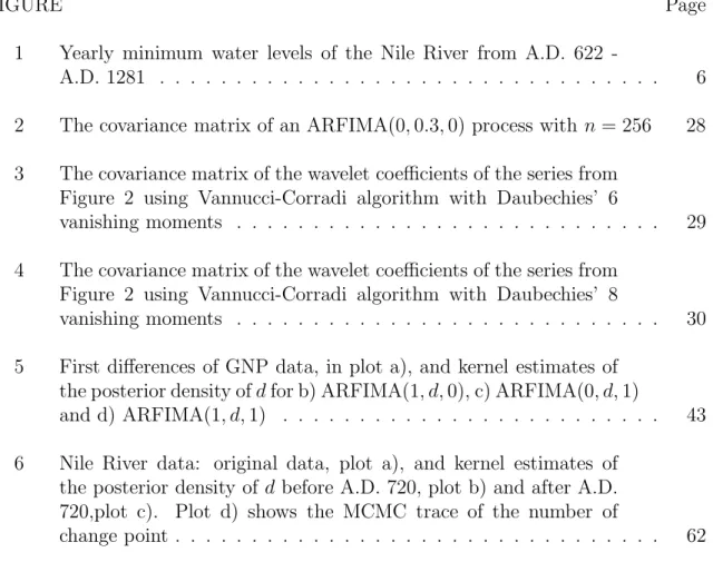
1 Yearly minimum water levels of the Nile River from A.D. 622
-A.D. 1281 . . . 6 2 The covariance matrix of an ARFIMA(0,0.3,0) process with n= 256 28 3 The covariance matrix of the wavelet coefficients of the series from
Figure 2 using Vannucci-Corradi algorithm with Daubechies’ 6
vanishing moments . . . 29 4 The covariance matrix of the wavelet coefficients of the series from
Figure 2 using Vannucci-Corradi algorithm with Daubechies’ 8
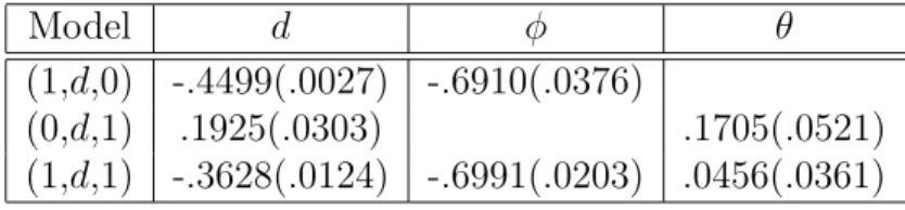
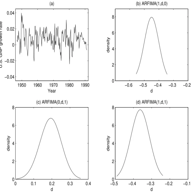
vanishing moments . . . 30 5 First differences of GNP data, in plot a), and kernel estimates of
the posterior density ofdfor b) ARFIMA(1, d,0), c) ARFIMA(0, d,1)
and d) ARFIMA(1, d,1) . . . 43 6 Nile River data: original data, plot a), and kernel estimates of
the posterior density of d before A.D. 720, plot b) and after A.D. 720,plot c). Plot d) shows the MCMC trace of the number of
LIST OF TABLES
TABLE Page
1 ARFIMA(1, d,0): Estimates ofdandφfrom wavelet-based Bayesian method with MP(7) wavelets, MLE and the Geweke and Porter-Hudak (1983) method, respectively. Numbers in parentheses are
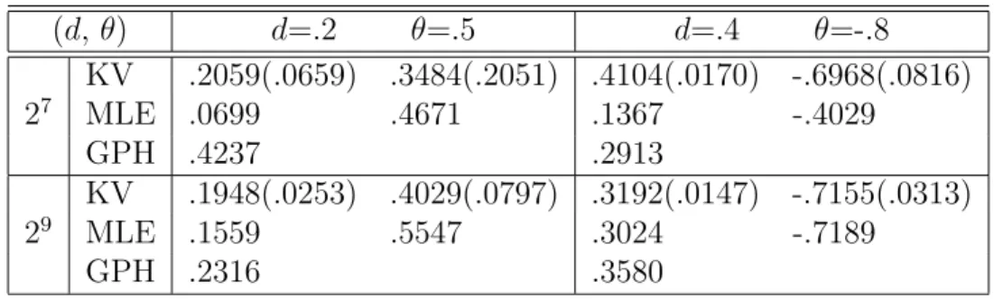
standard errors. . . 38 2 ARFIMA(0, d,1): Estimates ofdandθfrom wavelet-based Bayesian
method with MP(7) wavelets, MLE and the Geweke and Porter-Hudak (1983) method, respectively. Numbers in parentheses are
standard errors. . . 39 3 ARFIMA(1, d,1): Estimates ofd, φandθfrom wavelet-based Bayesian
method with MP(7) wavelets, MLE and the Geweke and Porter-Hudak (1983) method, respectively. Numbers in parentheses are
standard errors. . . 40 4 Wavelet-based Bayes estimates for U.S. GNP data . . . 41 5 Simulation result when diagonal elements and full matrix of ΣW
used in the estimation of long memory parameter of ARFIMA(0, d,0) model with sample size n = 128. The numbers in parenthesis
de-note biases. . . 45 6 Simulation result when diagonal elements and full matrix of ΣW
used in the estimation of long memory parameter of ARFIMA(0, d,0) model with sample size n = 512. The numbers in parenthesis
de-note biases. . . 46 7 Posterior probability of the number of change pointsk in the
sim-ulation of ARFIMA(1, d,1) model with φ=0.1, d1=0.2, d2=0.4,
θ=0.5 and one change point c=256 . . . 56 8 Parameter estimates of ARFIMA(1, d,1) model in the case of ˆk = 1. . 56 9 Posterior probability of the number of change pointskin the
simu-lation of ARFIMA(1, d,0) model with φ=0.3, d1=0.2, d2=0.3 and
TABLE Page 10 Parameter estimates of ARFIMA(1, d,0) model from simulated
data in the case of ˆk = 1. . . 57 11 Posterior probability of the number of change pointsk in the
sim-ulation of ARFIMA(0, d,1) model with d1=0.2, d2=0.3, θ = 0.3
and one change point c=256. . . 58 12 Parameter estimates of ARFIMA(0, d,1) model from simulated
data in the case of ˆk = 1. . . 58 13 Posterior probability of the number of change pointskin the
simu-lation of ARFIMA(1, d,1) model with φ= 0.1,θ = 0.4,d1 = 0.05,
d2 = 0.35, d3 = 0.45 and two change points at c1 = 128 and c2 = 256. 59 14 Parameter estimates of ARFIMA(1, d,1) model from simulated
data in the case of ˆk = 2.. . . 59 15 Posterior probability of the number of change pointsk in the Nile
River data using ARFIMA(0, d,0) model. . . 61 16 Parameter estimates of ARFIMA(0, d,0) model in the Nile River
CHAPTER I
INTRODUCTION
Long memory processes have been widely used in many fields, such as economics, finance and telecommunications to model characteristic phenomena. Most remarkable characteristics of long memory process compared to short memory is that dependen-cies between distant observations are not negligible. Common models for long mem-ory behavior are the fractional Brownian motion (fBm) and fractional Gaussian noise (fGn). Commonly used long memory processes in time series are the ARFIMA(p, d, q), first introduced by Granger and Joyeaux (1980) and Hosking (1984). For these mod-els the value of the spectral density function goes to infinity as the frequency goes to zero and classical time series methods for estimation and testing cannot be applied. Also, the structure of the variance-covariance matrix makes inferential methods com-putationally expensive and causes inaccurate estimates.
In early stage of the parameter estimation of Gaussian ARFIMA(p, d, q) mod-els, approximate maximum likelihood methods were used by Li and McLeod (1986) and Fox and Taqqu (1986), but these methods showed inaccuracy for finite samples. Sowell (1992a) calculated the exact form of the variance-covariance function to com-pute the likelihood function under the assumption that the roots of an autoregressive polynomial are simple, that is, the roots do not have repeated roots. This exact like-lihood method achieved accuracy, but is computationally exhaustive. Beran (1994) investigated asymptotic sampling theory properties of exact and approximate
imum likelihood methods. As for Bayesian approaches, Pai and Ravishanker (1996; 1998) adopt the Metropolis algorithm to estimate the model parameters and Koop et al. (1997) used importance sampling with the exact form of the variance-covariance matrix of Sowell (1992a).
While estimation of model parameters has been widely investigated, little work has been done in designing methods for change point analysis of the long memory parameter in ARFIMA(p, d, q) models. Change points in a given series result from unexpected changes in the physical mechanism or environmental condition that gen-erate data. Routine estimation techniques for model parameters may be inaccurate when change points are not properly located. Beran and Terrin (1996) proposed a test for detecting a single change in ARFIMA(p, d, q) model. Whicher, Guttorp and Percival (2000) used Iterative Cumulative Sums of Squares (ICSS) algorithm to test and locate multiple change points in variances of fractional difference process. They took discrete wavelet transform (DWT) of Gaussian I(d) processes to use ICSS which needs independently and identically distributed normal random variables for data. However, their method can only estimate the number of multiple change points and locate them without estimating the values of long memory parameterdt
correspond-ing to the detected change points. Ray and Tsay (2002) studied multiple change points analysis of the mean level and the long memory parameter. They considered ARFIMA(0, d,0) models only and used a time-dependent Kalman filter approach with a truncated MA approximation to evaluate the likelihood. Their method allows accurate estimation only if the change points occur at the ends of pre-specified data blocks. Moreover, they used a griddy Gibbs sampler algorithm to estimate the long memory parameter, a procedure that can lead to inaccurate estimates. Also, they used Bayes factor to assess proper number of change points. An alternative Bayesian method for multiple change point analysis was proposed by Liu and Kao (1999).
They adopted griddy Gibbs sampler algorithm but allowed the number of change points to be unknown and used the reversible jump MCMC of Green (1995). These authors considered the special case of ARFIMA(1, d,0) models with conditionally heteroscedastic innovations.
Wavelets have been known as a powerful tool for the analysis and synthesis of data from long memory processes. The ability of the wavelets to simultaneously lo-calize a process in time and scale domain results in representing many dense matrices in a sparse form. When transforming measurements from a long memory process, wavelet coefficients are approximately uncorrelated, in contrast with the dense long memory covariance structure of the data, see Tewfik and Kim (1992). This prop-erty of wavelet transform enables us to simplify dense covariance structure of data following ARFIMA(p, d, q) model into sparse form which we may regard as approxi-mately uncorrelated and thus may use relatively simple likelihood function. McCoy and Walden (1996) used this wavelet property to estimate ARFIMA(0, d,0) or I(d) models with approximate wavelet coefficients-based maximum likelihood iterative pro-cedure. Jensen (1999) proposed wavelet-based ordinary least squares estimate of the long memory parameter in I(d) process and compared his results to those by Geweke and Porter-Hudak (1983) and McCoy and Walden (1996). Also, Jensen (2000) pro-posed an alternative maximum likelihood estimator of ARFIMA(0, d,0) models using compactly supported wavelets.
We here propose an estimation procedure of the model parameters in Gaussian ARFIMA(p, d, q) models and a change point analysis of the long memory parameter in Gaussian ARFIMA(p, d, q) models with unknown multiple change points. In order to handle the dense covariance matrix of ARFIMA(p, d, q) models, we transform the original data into wavelet coefficients using discrete wavelet transform (DWT). A Metropolis algorithm is implemented in the wavelet domain for Bayesian estimation
of the model parameters. For the change point analysis, the reversible jump Markov chain Monte Carlo proposed by Green (1995) is adopted to estimate the unknown number of multiple change points and their locations together with the estimation of other model parameters. For both methods we use Vannucci and Corradi’s (1999) algorithm to transform the variance-covariance matrix in the time domain into the corresponding matrix in the wavelet domain.
In Chapter II we introduce the concept and class of long memory process and estimation procedures of long memory processes on literature. Basics of wavelets and relationship between long memory process and wavelet transforms are described in Chapter III. As a preliminary step for change point analysis, we develop a Bayesian estimation method of the parameters of ARFIMA(p, d, q) models on wavelet domain in Chapter IV. In Chapter V we propose a wavelet-based Bayesian change point analysis of the long memory parameter of ARFIMA(p, d, q) processes.
CHAPTER II
LONG MEMORY PROCESSES
2.1 Introduction
Standard time series analysis is concerned with series having the property that two observations separated by a long time interval are completely or nearly inde-pendent. However, there are many cases were we should not ignore the dependence between distant observations,even if it is small. It is said that a series having charac-teristic has ”long memory (or long range dependence)”. We can find this phenomenon in many fields such as economics, finance, hydrology and engineering. If we apply standard statistics to data having long memory the results may misguide us to wrong decisions. The reason is that variance of the sample mean of such series is not equal to σ2/n and thus routine estimation, such as interval estimation and testing about population mean, cannot be used.
In general, we can classify the memory type of a given time series in three ways: no memory, short memory and long memory. No memory series has no pattern over time and knowing the past of the series provides no information about its behavior in the future except for mean and variance. A white noise is a typical case of no memory. On the contrary, time series possessing short memory has exponentially decaying autocorrelation function. ARMA(p, q) processes are short memory processes. Long memory process can be non-stationary but typically it is predictable. In this case we need to identify some transformations to reduce the process to short memory type-process and then model the process by a whitening filter to have no memory residuals.
700 800 900 1000 1100 1200 900 1000 1100 1200 1300 1400 1500 year
yearly minimum water level
Figure 1: Yearly minimum water levels of the Nile River from A.D. 622 - A.D. 1281
2.2 Features and definition of long memory processes
The qualitative behavior of a long memory process, for which the first two mo-ments exist, can be described as follows. First, the path of series look like stationary. Second, there is no lasting cycle or trend through the whole series although we could find cycles or local trends on short time periods of the path. A typical example show-ing these features is the Nile River data (A.D. 622-A.D. 1281). If we have a closer look at a short time period of Figure 1 then we could find cycles or trends but we cannot find those patterns in the whole series. On the other hand, quantitative properties of a long memory process are (i) the variance of the sample mean of this process decays to zero at a slower rate thann−1 and (ii) the sample correlations decay hyperbolically to zero. These are main differences between short and long memory processes.
There are some mathematical definitions of a long memory process with station-arity in terms of autocovariance and spectral density.
Definition 2.2.1 Suppose that Xt is a process with autocovariance function γ(τ)∼
C(τ)τ2d−1 as τ → ∞, C(τ) 6= 0. Then we call X
Moreover, if 0< d <0.5 then the process is stationary.
Here C(τ) does not depend on dand is a slowly varying function as |τ| → ∞ (Beran and Terrin, 1996). The d is called long memory(or long range) parameter. From the definition 2.2.1, we know that the correlations are not summable. Some authors give further distinction according to the range of d, that is, if d < 0 and hence P∞
τ=−∞|γ(τ)|<∞then the process is “intermediate” and the process is “long mem-ory” if 0< d <0.5 and hence P∞τ=−∞|γ(τ)|=∞. The following definition describes the property of long memory in terms of the spectral density.
Definition 2.2.2 Suppose that a processXt has the spectral density such thatf(λ)∼
k(λ)λ−2d as λ → 0. Then we call X
t a stationary process with long memory if
0< d < 0.5.
From the definition 2.2.2 the spectral density of a process with long memory has a pole at zero.
The hydrologist Hurst (1951) proposed the so-called “Hurst” (or self-similar) parameter, H, which has a simple relationship with the long memory parameter, that is H = d+ 1
2. He noticed that the rescaled adjusted range, R/S statistic, has asymptotically a log linear relationship with the sample size and a slope H larger than 12.
2.3 Class of stationary process with long memory
A stationary process with long memory can be classified in two ways, continuous and discrete time. In the continuous time domain, we have three processes with long memory: self-similar process, fractional Brownian motion (fBm) and fractional Gaus-sian noise (fGn). A typical discrete long memory process is the fractional ARIMA. Self-similar and ARFIMA(0, d,0) processes are the basic processes of continuous and discrete long memory processes, respectively.
2.3.1 Continuous long memory process
Fractional Brownian motion and fractional Gaussian noise belong to continuous long memory process. They can be formulated from self-similar process.
Definition 2.3.1 A stochastic process,Xt with continuous time parameter such that
c−HX
ct=d Xt is called self-similar with self-similarity parameter H.
Here “=d” means “equal in distribution”. A real-valued process {X
t, t ∈ T} has
stationary increments if {Xt+h −Xh, t ∈ T} =d {Xt −X0, t ∈ T} for all h ∈ T.
Then a Gaussian self-similar process {BH(t)} with stationary increments is called
fractional Brownian motion when its self-similarity parameter, H is in (0,1). When var(BH(1)) =σ2, the autocovariance function is
γ(s, t) = cov(BH(s), BH(t)) =.5σ2[t2H −(t−s)2H +s2H], s < t.
Thus fBm has stationary increments but is not stationary process. Let’s define a increment process ofBH(·) asYt =BH(t+ 1)−BH(t) which is a stationary sequence.
We callYt fractional Gaussian noise. The covariance function of the increment process
is
γ(τ) = cov(Yt, Yt+τ) =.5σ02[(τ + 1)2H −2τ2H + (τ −1)2H], (2.1) whereEY2
t =EBH(1)2 =σ02. Also we know that fGn is a stationary process because (2.1) does not depend on t. The correlation function of Yt is calculated by
ρ(τ) =γ(τ)/γ(0) =.5[(τ+ 1)2H −2τ2H + (τ −1)2H] Asτ → ∞, using Taylor’s expansion,
ρ(τ)∼H(2H−1)τ2H−2. (2.2)
Thus fGn is long memory process. The correlations are not summable for 0.5< H < 1 (0 < d < 0.5) in which Yt has long memory, summable for 0 < H < 0.5 (−0.5 <
2.3.2 Discrete long memory process
The simplest of ARFIMA(p, d, q) models is ARFIMA(0, d,0) model which is also called integrated process I(d). A process {Xt}t∈Z is called ARFIMA(0, d,0) model if
it has relationship (1−B)dX
t =εt for any reald >−0.5, whereεt is zero mean white
noise with innovation varianceσ2. Fractional difference operator ∆d = (1−B)d where
B is backshift operator can be defined as power series in B for d 6= 0. By binomial expansion, for any real number d,
(1−B)d ≡ ∞ X j=0 πjBj = ∞ X j=0 d j (−1)jBj, (2.3)
where dj=d!/j!(d−j)! = Γ(d+ 1)/Γ(j+ 1)Γ(d−j+ 1). This comes from the fact that gamma function is defined for all real numbers and the binomial coefficient can be extended to all real number d. Since πj = (−1)j dj
can be approximated as (−1)j d j = (−1)j Γ(d+ 1) Γ(j + 1)Γ(d−j+ 1) = (−1)j(−1) j(−d)(−d+ 1)· · ·(−d−1 +j) Γ(j + 1) = (−1)j(−1) jΓ(−d+j) Γ(j + 1)Γ(−d) = Γ(−d+j) Γ(j+ 1)Γ(−d) ∼ j−d−1/Γ(−d) as j → ∞,
the I(d) process can be expressed as an AR(∞) of the form (1−B)dXt =εt ⇒
∞ X
j=0
j−d−1/Γ(−d)BjXt =εt as j→ ∞ (2.4)
under the condition such thatP∞j=1π2 <∞ in (2.4). Since π2
j ∼j−2d−2/Γ2(−d), for
the convergence of the summation, dshould satisfy −2d−2<−1 ⇒ −2d <1
Thus I(d) process or ARFIMA(0, d,0) model is invertible ifd >−0.5. For the condi-tion such that{Xt}t∈Z is stationary process, assume that ∆dXt =εt be inverted into
Xt = ∆−dεt. Since ∆−d = (1−B)−d ≡P∞j=0ψjBj =P∞j=0 −jd (−1)jBj and (−1)j −d j = (−1)j Γ(−d+ 1) Γ(j + 1)Γ(−d−j+ 1) = (−1)j(−1) j(d)(d+ 1)· · ·(d+j−1) Γ(j + 1) = (−1)j(−1) jΓ(d+j) Γ(j+ 1)Γ(d) = Γ(d+j) Γ(j + 1)Γ(d) ∼ jd−1/Γ(d) as j→ ∞,
the inverted process can be expressed as an MA(∞) of the form (1−B)dXt =εt ⇒ Xt = ∆−dεt ⇒ Xt = ∞ X j=0 ψjεt−j, (2.5)
under the condition such thatP∞j=1ψ2
j <∞in (2.5). Since ψj2 ∼j2d−2/Γ2(d), for the
convergence of the summation, we also need a condition for d such that 2d−2<−1 ⇒ 2d <1
⇒ d <0.5.
So ARFIMA(0, d,0) model is stationary if d < 0.5. Therefore, ARFIMA(0, d,0) model is invertible and stationary if d ∈ (−0.5,0.5). In the case of d ∈ (−0.5,0.5), {Xt}t∈Z has the spectral measure dZX(λ) = |B(λ)|dZε(λ) = (1−e−iλ)−ddZε(λ) and
the spectral density fX(λ) = B(λ)2dZε(λ) = |1−e−iλ|−2dσ 2 2π = |2sin(λ/2)|−2dσ 2 2π ∼ σ 2 2π|λ| −2d, λ →0, (2.6)
where σ2 is the white noise variance. Thus from definition (2.2.2) ARFIMA(0, d,0) process has long memory.
A time series,{xt}t∈Z, is said to be fractionally differenced autoregressive moving
average model if the series is identified as an ARMA(p,q) model after applying the fractional difference operator (2.3). The general fractionally differenced ARMA(p, q) model can be written as
Φ(B)(1−B)dXt = Θ(B)εt, (2.7)
where
Φ(B) = 1 +φ1B+φ2B2+· · ·+φpBp
and
Θ(B) = 1 +θ1B+θ2B2+· · ·+θqBq
are polynomials in the backshift operatorB and εt is a white noise process with zero
mean and variance σ2. We denote the above as ARFIMA(p, d, q) model. The model (2.7) can be rewritten by
Φ(B)Xt = Θ(B)Ut and Ut = (1−B)−dεt. (2.8)
Thus we can regard ARFIMA(p, d, q) process as ARMA(p, q) process driven by I(d) process,Ut = (1−B)−dεt. Since ARMA(p, q) model is typical short memory process
in time series and I(d) process has long memory, the long term behavior is determined bydand the short term behavior is determined byφandθ in ARFIMA(p, d, q) mod-els. That is, d and (φ, θ) describe the high-lag and low-lag correlation structures of ARFIMA(p, d, q) models. Thus the long-term behavior of ARFIMA(p, d, q) models may be similar to the one of ARIMA(0, d,0) because the influence of the φ’s and θ’s is negligible for distant observations. From this fact, the ARIMA(p, d, q) process has long memory if d ∈ (−0.5,0.5) and in addition, is weak stationary and invert-ible if and only if the roots of Φ(z) and Θ(z) are outside the unit circle. Geweke and Poter-Hudak (1983) used two-step procedures with the two models in (2.8) to estimate the model parameters of ARFIMA(p, d, q) models. Hosking (1984) proposed the algo-rithm for simulating an ARFIMA(p, d, q) process with the same notion, which is (i) to generateUt from ARFIMA(0, d,0) and (ii) to generateXt usingUt from ARMA(p, q)
process.
Since the spectral measure of{Xt}t∈Z in (2.7) is dZX(λ) = θ(e−iλ)φ(e−iλ)−1(1−
e−iλ)−ddZ
ε(λ) whereθ(λ) = Θ(e−iλ) andφ(λ) = Φ(e−iλ) are transfer functions related
to AR and MA terms, its spectral density and asymptotic autocovariance function are f(λ) = σ 2 2π |θ(e−iλ)|2 |φ(e−iλ)|2|1−e −iλ |−2d ∼ σ 2 2π |θ(1)|2 |φ(1)|2|λ| −2d , as λ →0 (2.9) and γ(τ)∼Cτ2d−1 as τ → ∞, (2.10)
where C 6= 0 and does not depend on τ. On the other hand, under the additional assumption that the roots of Φ(z) are simple, Sowell (1992a) showed that the
auto-covariance function of this process is γ(τ) =σ2 q X l=−q p X j=1 ψ(l)ζjC(d, p−τ+l, ρj) (2.11) where ψ(l) = minX[q,q−l] τ=max[0,l] θτθτ−l, ζj = [ρj p Y i=1 (1−ρiρj) Y m6=j (ρj −ρm)]−1, and C(d, h, ρ) = Γ(1−2d)Γ(d+h) Γ(1−d+h)Γ(1−d)Γ(d) ×[ρ2pF(d+h,1; 1−d+h;ρ) +F(d−h,1; 1−d−h;ρ)−1]. Here F(a,1;c;ρ) is the hypergeometric function and has the recursive relationship
F(a,1;c;ρ) = c−1
ρ(a−1)[F(a−1,1;c−1;ρ)−1].
For ARFIMA(0, d, q) model i.e. p= 0, the autocovariance function has the form γ(τ) =σ2 q X l=−q ψ(l) Γ(1−2d)Γ(d+l−τ) Γ(1−d+l−τ)Γ(1−d)Γ(d). (2.12) Moreover, forp=0 and q=0 in ARFIMA(p, d, q) model, it becomes
γ(τ) =σ2 Γ(1−2d)Γ(d+τ) Γ(1−d+τ)Γ(1−d)Γ(d).
These processes are stationary if d < 0.5 and possess invertibility or AR(∞) repre-sentation if d > −0.5. Also, they have long memory for 0 < d < 0.5, short memory for d= 0 and intermediate for −0.5< d <0. Sowell (1992a) use the Levinson algo-rithm to reduce the order of calculating the likelihood function by decomposing the covariance.
2.4 Heuristic estimation of long memory parameter
Given a series we need to know if it has long memory. For this purpose we can use some heuristic methods based on the properties and definitions of long memory mentioned in previous section. The most basic checking method for long memory is to investigate whether the ACF plot decays hyperbolically to zero. Other heuristic methods are based on plots of basic statistics in log scale and least square fits of them. 2.4.1 the R/S statistic versus k
Let Xi denote a value of given process at time i and define Yj = Pji=1Xi. The
modified rangeR(t, k) and its scaling factor S(t, k) are defined as follows. R(t, k) = max0≤i≤k[Yt+i−Yt− i k(Yt+k−Yt)]−min0≤i≤k[Yt+i−Yt− i k(Yt+k−Yt)] and S(t, k) = [k−1 t+k X i=t+1 (Xi−X¯t,k)2]1/2
In the plot of log[R(t, k)/S(t, k)] versus logk, the points are scattered around a straight line of slope 0.5 for i.i.d. series and are scattered around a straight line of slope greater than 0.5 for long memory processes. That is, in the least square line of logE(R/S)≈c+Hlogk, if H≈0.5 then the process is i.i.d.and if H >0.5 then the process has long memory.
2.4.2 Sample variance versus its sample size
The variance of the sample mean of long memory process decays to zero at a slower rate thann−1. So plotting sample variance versus sample size in log scale and fitting a least square line can be used for the estimation of long memory parameter. If the slope of the line is far from -1 then we conclude this process has long memory.
Actually the slope -1 is a theoretical value for summable correlations. Also if corre-lations are summable the periodogram ordinates near the origin should be scattered randomly around a constant.
2.4.3 Correlogram
From definition 2.2.1 we might draw a plot of ρ(τ) = γ(τ)/γ(0) versus τ in log scale and fit a least square line. If the slope is between -1 and 0 we conclude that the series exhibits long range dependence.
2.5 Semi-parametric estimation: Geweke and Porter-Hudak’s estimate
Definition 2.2.2 needs to be carefully understood in that the spectral density is proportional toλ−2donly in a neighborhood of zero. Geweke and Porter-Hudak (1983)
used this notion to get a least square estimate of long memory parameter d at low frequencies in the case of integrated models I(d). They used the periodogram I(λ) and the Fourier frequencies λi,n as the sample estimates of the spectral density and
frequencies, respectively in the equation taking logarithm of the asymptotic relation off(λ). This leads to
logI(λi,n)≈logk−2dlogλi,n+ logεi (2.13)
If the least square estimate of the slope in the equation (2.13) is ˆβ then the estimate of long memory parameter is
ˆ d=−βˆ
2
GPH estimator has been widely used with desirable precision in estimation of long memory parameter by virtue of its simplicity and computational speed. For fractional ARFIMA(p, d, q) models Geweke and Porter-Hudak also proposed two-step estimation procedures where the d is estimated under the model I(d), the data is transformed
intoYt = (1−B)dˆand standard ARMA models are applied to the transformed Ut in
order to estimate AR and MA parameters and identify the orders.
2.6 Parametric estimation of long memory parameter
Suppose that an ARFIMA(p, d, q) model is fitted to a Gaussian process {Xt}
with size n. Then the likelihood function is L(Ψ) = (2π)−n/2|Σ(Ψ)|−1/2exp −12X0Σ(Ψ)−1X , (2.14) where Ψ = (σ2
ε, d, φ1, . . . , φp, θ1, . . . , θq), σε2 is the innovation variance in (2.7) and
Σ(Ψ) is the n×n covariance matrix of X. The MLE, ˆΨ, is the value of maximizing L(Ψ) or minimizingl(Ψ) =−2logL(Ψ). If we define the (p+q+2)-dimensional vector
l0(Ψ) = ∂ ∂Ψl
0(Ψ), (2.15)
then the MLE, ˆΨE under mild regularity condition is the solution of the system of
(p+q+ 2)-equations
l0( ˆΨ) = 0. (2.16)
Yajima (1985) proves the limit theorem of ˆΨ in the case of ARFIMA(0, d,0) process and Dahlhaus (1989) shows the result for ARFIMA(p, d, q) model. If the dimension of Ψ is large or the data sizen is big enough then the calculation of the exact MLE is computationally intensive because the likelihood function (2.14) is the implicit func-tion of Ψ through the covariance matrix Σ(Ψ) and thus (2.16) should be evaluated for many trial values of Ψ. The other problem is to get the inverse of the covariance matrix, Σ(Ψ)−1. Note that a large number of data is needed to estimate the long memory parameter with desirable precision because it describes the long-term per-sistence between distant observations. The inversion of a large size of the covariance may be numerically unstable.
An alternative method to avoid those problems is to use an approximation to the likelihood function. Alln×n symmetric Toeplitz matrices have complex orthonormal eigenvectors and the corresponding eigenvalues which can be well approximated by
Vj =
√
n−1{exp(−iλ
jt)}t=1,...,n−1 and Γj ={2πfΨ(λj)}, j = 1, . . . , n−1,
where Vj is jth column vector of complex eigenvector matrix V, Γj is jth diagonal
element of the diagonal matrix Γ and fΨ(λ) is the spectral density of the process. Thus
Σ(Ψ)≈VΓVc, (2.17)
whereVc is the conjugate transpose of V. Thus
l(Ψ) = nlog(2π) + log|Σ(Ψ)|+X0Σ(Ψ)−1X ≈ nlog(2π) + log|VΓVc|+X0VΓ−1 VcX0 (2.18) = nlog(2π) + n−1 X j=1 [log(2πfΨ(λj)) +n|J(λj)|2/(2πfΨ(λj))] = 2nlog(2π) + n−1 X j=1 [logfΨ(λj) +I(λj)/fΨ(λj)], (2.19)
where I(λj) is the periodogram of Xt and J(λj) = n−1Pnt=0−1Xtexp(−iλjt) which
is the discrete Fourier transform of Xt. Note that X0V = √n(J(λ0), . . . , J(λn−1))
because X0Vj = √ n−1 n−1 X t=0 Xtexp(−iλjt) = √nJ(λj).
The estimate, ˆψW which minimize (2.18) is called Whittle’s approximate MLE. Fox
CHAPTER III
WAVELETS
3.1 Introduction
Wavelets are relatively new mathematical tools for time series analysis and image analysis. Wavelet means “small wave”. On the contrary, examples of “big waves” are sine and cosine function usually used for Fourier analysis. Wavelets are the building blocks of wavelet transformations in the same way as the functions einx =
cos(nx) +isin(nx) are the building blocks of the Fourier transformation.
Wavelet methods are used in statistics for smoothing of noisy data, nonparamet-ric density and function estimation, and stochastic process representation. A popular application in nonparametric statistics is wavelet shrinkage, which can be described as 3 step procedure: (i) the original series is transformed into a set of wavelet coeffi-cients, (ii) a shrinkage of those coefficients is applied, and (iii) the resulting wavelet coefficients are transformed back to the original data domain. Nowadays the appli-cation of wavelets in statistics is rapidly growing and expanding to other areas like economics, finance and so on.
Wavelet theory is similar to Fourier analysis but it has a critical advantage. Wavelet transforms well localize original series in both time and frequency (scale) domains, while Fourier transforms do so only in the frequency domain. Thus one loses time information through Fourier transform but not via wavelet transform.
3.2 Prerequisites
Here some useful mathematical definitions related to wavelet theory are de-scribed. In wavelet theory we deal with functions in L2(R) and `2(R).
Definition 3.2.1 The space of all square integrable functions is called L2(R). That is, f(x)∈L2(R) if R |f(x)|2 <∞.
The inner product of two functions and norm of a function in L2(R) are defined as < f, g >=R f g and kfk=qR f2, respectively.
Definition 3.2.2 The space of all square summable sequences is called `2(R). That is, x1, . . . , xn ∈`2(R) if
Pn
i=1x2i <∞.
The inner product of two sequences and norm of a sequence on `2(R) are defined as < x,y >= Pni=1xiyi and kxk = pPni=1xi2, respectively. The following definition
plays an important role in wavelet decomposition and synthesis.
Definition 3.2.3 Suppose that V is an inner product space and W a finite dimen-sional subspace ofV. For v ∈V, the orthogonal projection of v ontoW is the unique vector v0 ∈W such that
kv−v0k=minw∈Wkv−wk.
Here the orthogonal complement of W in V, W⊥ is defined as W⊥ = {v ∈ V| < v, w >= 0}for allw∈W. We can representV as the orthogonal sum of W and W⊥, V =W ⊕W⊥.
3.3 Basics of a wavelet decomposition
There are two basic functions in wavelet analysis, the scaling function φ(x) and the (mother) wavelet functionψ(x). Sometimes φ(x) is called “father wavelet”. The building blocks to approximate a given function are constructed by the translations and dilations of the scaling function. Note that the translationφ(x−k) has the same shape asφ(x) except translated by kunits and the dilationφ(2jx) has the same shape
is the Haar scaling function defined as φ(x) = 1 if 0≤x <1 0 otherwise (3.1)
Let Vj be the space of all functions of the form Pk∈Zakφ(2jx−k), j > 0, ak ∈ R
andk is a finite set of integers. In other words, Vj is defined to be the space spanned
by the set
{. . . , φ(2jx+ 2), φ(2jx+ 1), φ(2jx), φ(2jx+ 1), φ(2jx+ 2), . . .}.
Thus Vj is the space of piecewise constant functions with finite support whose
dis-continuities are in the set {. . . ,−2/2j,−1/2j,0,1/2j,2/2j, . . .}. Any function in V
0
is contained in V1 and likewise V1 ⊂ V2. The following hierarchical relation is estab-lished.
. . . V0 ⊂V1 ⊂. . .⊂Vj−1 ⊂Vj ⊂Vj+1. . . (3.2) Vjcontains all relevant informations up to a resolution scale 2−j. The larger getsj, the
finer is resolution. We know from the containment that information is not lost as the resolution gets finer. The collection of functions φj,k(x) = {2j/2φ(2jx−k);j, k ∈ Z}
is an orthonormal basis ofVj.
The mother wavelet functionψ(x) enters into wavelet decomposition of an origi-nal functionf to catch “spikes” which belong toVj and do not belong toVj−1. SoVj is
decomposed as an orthogonal sum ofVj−1and its orthogonal complementWj−1, which
is denoted by Vj = Vj−1⊕Wj−1 where < vj−1, wj−1 >= 0, vj−1 ∈ Vj and wj−1 ∈ Wj−1. The orthogonal complement of Vj, Wj−1 is generated by the translations and dilations ofψ(x) as ifVj is done by the translations and dilations of φ(x). As in the
case of φj,k(x), the collection of functions ψj,k(x) = {2j/2ψ(2jx−k);j, k ∈ Z} is an
functionψj,k(x), which are (i) R∞ −∞ψj,k(x)dx= 0 and (ii) R∞ −∞ψj,k(x) 2dx= 1, ∀j, k ∈
Z. The simplest mother wavelet function is the Harr wavelet which is defined by
ψ(x) = 1 if 0≤x <1/2 −1 if 1/2≤x <1 0 otherwise (3.3)
Note that the Haar wavelet function (3.3) can be denoted by a linear combination of the Haar scaling functions (3.1) as ψ(x) =φ(2x)−φ(2x−1).
The main idea of wavelet decomposition is to orthogonally project a given func-tion f ∈ L2 onto the space of scaling functions at a resolution j, say Vj, which is
f 'fVj =
P
k∈Zcj,kφj,k(x). Then fVj is again decomposed into the space of the next
coarser scaleVj−1 through the relation (3.2). This is the main stem of multiresolution analysis (MRA) by Mallat (1989).
3.4 Multiresolution analysis
A multiresolution analysis (Mallat, 1989) is a framework for creating general φ and ψ. MRA is a decomposition of a function in L2 into scaling basis φj,k(x) and
wavelet basisψj,k(x). It is an embedded grid of approximation by (3.2).
Approxima-tion off ∈L2 at a resolution j is an orthogonal projection fj off onVj, which means
thatkf −fjk is minimized (Definition 3.2.3).
Definition 3.4.1 A sequence{Vj}j∈Z of subspaces of functions inL2 is called a mul-tiresolution analysis with scaling function φ if the following properties holds.
(1) Vj ⊂Vj+1, ∀j ∈Z
(2) ∪j∈ZVj =L2 and ∩j∈ZVj =φ
(3) f(x)∈Vj if and only if f(2x)∈Vj+1, ∀j ∈Z
(4) f(x)∈V0 if and only if f(x+k)∈V0, ∀k∈Z
for V0.
The {Vj}j∈Z’s are also called approximation spaces. The only condition for choosing
a φ is that the set of its translations, {φ(x−k);k ∈ Z} is a basis. Generally the most useful property of scaling functions is to have compact support which means that a function has identically zero outside of a finite interval andcontinuity because a scaling function having these two properties has faster computing time and better performance for decomposition or reconstruction.
Suppose that{Vj}j∈Z is a multiresolution analysis with scaling functionφ. Then
φj,k(x) = {2j/2φ(2jx−k);k ∈ Z} is an orthonormal basis for Vj. Also the following
two central equations in multiresolution analysis hold.
• (Two-scale equation)There exists{hk}k∈Zsuch thatφ(x) =
P
k∈Zhk21/2φ(2x
−k) = Pk∈Zhkφ1,k, where hk =< φ(x), φ1,k >∈ `2(R). {hk} is called low-pass
filter(or scaling filter).
• (Wavelet equation)There exists{gk}k∈Zsuch thatψ(x) =
P
k∈Zgk2
1/2φ(2x− k) = Pk∈Zgkφ1,k, where gk =< ψ(x), φ1,k >∈ `2(R). {gk} is called high-pass
filter(or wavelet filter).
The above two equations are forms of convolution with filter coefficients {hk} and
{gk}, respectively. The inner products are performed according to the Definition 3.2.1
or 3.2.2 depending on the attribute of x. From the two central equations, it can be shown that ψj,k(x) = {2j/2ψ(2jx−k);k ∈ Z} is orthonormal basis for Wj which is
the orthogonal complement ofVj in Vj+1. By successive orthogonal decompositions,
Vj+1 = Wj⊕Vj
= Wj⊕Wj−1⊕Vj−1 = . . .
= Wj⊕Wj−1⊕ · · · ⊕W1⊕W0⊕V0 (3.4) If{Vj}j∈Z is a multiresolution analysis with scaling function φ and Wj is the
orthog-onal complement ofVj in Vj+1, then
L2(R) =· · · ⊕W−2⊕W−1⊕W0⊕W1⊕W2⊕ · · · . (3.5) Thereforef ∈L2(R) can be denoted by a unique sum ofwk ∈Wk, k ∈(−∞,∞) and
soψj,k(x) is an orthonormal basis for L2(R). 3.5 Discrete wavelet transform
For decomposition f ∈L2 is orthogonally projected on Vj, that is, f ≈fj ∈ Vj.
First decomposition is started withfj into a coarser approximation part, fj−1 ∈Vj−1 and wavelet(detail) part wj−1 ∈ Wj−1. From the equation (3.4), fj = fj−1 +wj−1. Then the decomposition is repeated with fj−1 and so on. Reconstruction algorithm is the reverse of decomposition.
There are two kinds of wavelet decomposition, continuous wavelet transform (CWT) and discrete wavelet transform (DWT). CWT is designed to decompose series defined over the entire real axis and DWT is used to transform series over a range of integers. Discrete wavelet transform is the basic tool for time series analysis and has an analogous feature to the discrete Fourier transform in spectral analysis. DWT has a property to effectively decorrelate highly correlated time series under certain condition and with this reason it is often used for time series analysis. Pyramid
algorithm (or Cascade algorithm) by Mallat (1989) is mainly used for discrete wavelet transform.
• (Pyramid algorithm) Given approximation coefficients at level j, wavelet and approximation coefficients of all coarser levels can be computed by iterative equations, cj,k = X l∈Z hl−2kcj+1,l dj,k = X l∈Z gl−2kcj+1,l (3.6)
Filter coefficients {gm} and {hm} is called high-pass filter and low-pass filter,
respectively. The relation between high-pass filter and low-pass filter is
gm = (−1)mh1−m. (3.7)
The equations (3.6) is simply a rephrase of the two-scale equation and wavelet equation.
The pyramid algorithm transforms original series X with length N = 2J into the
N/2’s wavelet coefficients W1 = {dJ−1,k;k = 1, . . . , N/2} and N/2’s scaling
coef-ficients V1 = {cJ−1,k;k = 1, . . . , N/2}. Then V1 is decomposed into W2 and V2 in the same ways as before. Repeated this way, J’s wavelet coefficient vectors W1,W2, . . . ,WJ and one scaling coefficient vector VJ are generated. Both Vj and
Wj, j = 1, . . . , J have the coefficients ofN/2j. Note thatW1 is the vector of wavelet coefficients with the highest resolution(or scale) and WJ is the one with the lowest
resolution(or scale). On the other hand, the subscripts ofcj anddj preserve the order
of resolution in the equation (3.4).
Each stage can be described in terms of filtering, that is, the elements of Vj
algorithm usesdownsampling(or decimation) method on each stage which is denoted by hl−2k and gl−2k instead of hl−k and gl−k in equations (3.6). Downsampling is a
mapping from`(Z) to`(2Z) which means that every other coefficients in Vj are used
for filtering to generate Vj+1 and Wj+1. It retains only the values of even indices
in sequences. Also it uses circular convolution for filtering of finite sequences. This circular convolution causes the coefficients affected by boundary condition.
3.5.1 Wavelet families and filters
There are several wavelet families such as Haar’s, Daubechies’s, Shannon’s and so on. Two important families are as follows.
• (Haar’s wavelets) This is the simplest wavelet family. It’s scaling function is (3.1). This can be rewritten in the form of
φ(x) = φ(2x) +φ(2x−1) = √1 2 √ 2φ(2x) + √1 2 √ 2φ(2x−1). (3.8)
From the two-scale equation, the scaling filters for the Haar’s family are h0 = h1 = √1
2. Since Haar’s wavelet function is ψ(x) = φ(2x)−φ(2x−1) = √1 2 √ 2φ(2x)− √1 2 √ 2φ(2x−1), (3.9)
the wavelet filters areg0 =−√1
2 andg1 = 1 √
2 from the wavelet equation or the equation (3.7). The Haar wavelets has compact support and are well localized in the time domain but discontinuous and so not effective in approximating smooth functions. The Haar wavelets satisfies three characteristics of wavelet basis functions which are compact support, orthogonality and symmetry.
• (Daubechies’ wavelets) Daubechies (1992) constructed the hierarchy of the compactly supported and orthogonal wavelets with a desired degree of smooth-ness (regularity). This smoothsmooth-ness can be set by the number of vanishing mo-ments which is defined thatψ(x) hasN (≥2) vanishing moments if< ψ(x), xn >
= 0, ∀n = 0,1, . . . , N −1. The simplest of Daubechies’ wavelets is the Haar wavelet which has zero vanishing moments. It is the only discontinuous wavelet of Daubechies’ ones. As the number of vanishing moments increases, the smooth-ness also does. There exists 2N’s nonzero, real scaling filters when the number of vanishing moments is N. Two kinds of Daubechies’ wavelets are the least asymmetric wavelets (symmlets) and the minimum phase wavelets.
3.5.2 Weakness of DWT
There exist some practical issues to be considered before using discrete wavelet transforms. Two major things are choice of width of the wavelet filter and handling boundary conditions.
• (Width of the wavelet filters) Width of wavelet filters is defined as the number of nonzero wavelet filters. For example, the width of Haar’s wavelet fil-ters is 2 and the one of Daubechies’s least asymmetric wavelets with vanishing moments of 3 is 6. Large width of wavelet filters can be (1) increasing coef-ficients affected by boundary conditions and computation time, (2) decreasing the degree of localization of the coefficients. So it is desirable to use the smallest width giving reasonable results.
• (Boundary condition) This is resulted from the circular filtering of the algo-rithm. Suppose that the width of given wavelet filters is L. Then the number of coefficients affected by boundary condition in Nj dimensional vectorWj can be
calculated by min{(L−2)(1−1/2j)}, N
j}. These are placed near the beginning
or end of the coefficients in each resolution. It is wise to proceed in statistical inferences after eliminating those affected by boundary conditions.
3.6 Variances and covariances of wavelet coefficients
For the matrix notation of the DWT suppose that a data vectorX= (X1, X2, . . . , XN where N = 2J is a realization of a random process {Xt : t = 1,2, . . .} with the
autocovariance function γ(t) = ΣX(i, j) where |i−j| = t. Also let’s {Wn : n =
0,1, . . . , N −1} consist of the DWT coefficients of original data vector X. Then we write W = WX where W is a column vector of length N = 2J whose nth element
is the nth DWT coefficients Wn and W is a N ×N orthogonal real-valued matrix
defining the discrete wavelet transform. The covariance matrix of the random process
X can be easily calculated from ΣX as
ΣW =WΣXW0, (3.10)
where ΣW is the variance-covariance matrix of the wavelet coefficients W and vice
versa. The covariance matrix, ΣW of a wavelet transform has the form of Toeplitz
matrices at different scales, while the covariance matrix is of Toeplitz form on time domain.
Vannucci and Corradi (1999) proposed an efficient algorithm to calculate ΣW
which uses the recursive filters in (3.6). This algorithm has a link to the two-dimensional discrete wavelet transform (DWT2). The DWT2 is first applied to ΣX.
Then the diagonal blocks of the resulting matrix give the variance-covariance matri-ces of wavelet coefficients that belong to the same scale which is called “within-scale” variance-covariance matrices. Next applying the one-dimensional DWT to the rows of the non diagonal blocks of the resulting matrix leads us to the “across-scale”
variance-covariance matrices which belong to different scales.
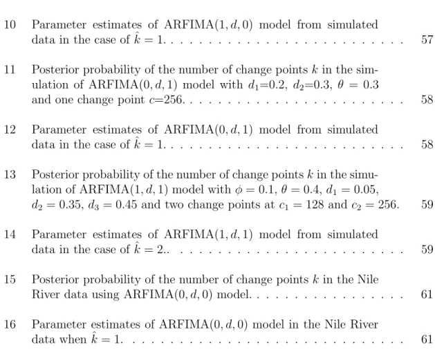
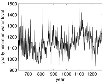
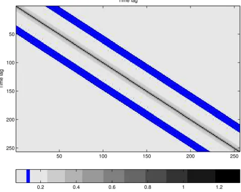
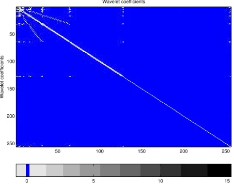
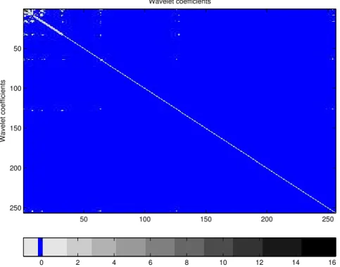
For example, Figure 2 shows the covariance matrix of a series with n = 256 from Gaussian ARFIMA(0,0.3,0) process using the Matlab function imagesc that displays matrices as images. The highest gray-scale values of the images correspond to the largest entries of the matrices. In the plot we can see that almost all entries of the covariance matrix of ARFIMA(0,0.3,0) process are away from zero, which means that the covariance matrix is dense. On the other hand, Figures 3 and 4 correspond to the covariance matrices of wavelet coefficients of the ARFIMA process with Daubechies’ 6 and 8 vanishing moments, respectively. We know that there is essentially no correlation among coefficients at the same scale but some correlation between scales, as shown by the extra-diagonal gray lines, but it decreases when using wavelets with higher numbers of vanishing moments.
Time lag Time lag 50 100 150 200 250 50 100 150 200 250 0.2 0.4 0.6 0.8 1 1.2
Wavelet coefficients Wavelet coefficients 50 100 150 200 250 50 100 150 200 250 0 5 10 15
Figure 3: The covariance matrix of the wavelet coefficients of the series from Figure 2 using Vannucci-Corradi algorithm with Daubechies’ 6 vanishing moments
3.7 DWT and long memory processes
In recent years discrete wavelet transforms of long memory processes have been popular because of their decorrelation properties and the simplification of the cor-responding likelihood on wavelet domain. Tewfik and Kim (1992) showed that the correlations between discrete wavelet coefficients from the models of fractional Brow-nian motion (fBm) decrease across scales and time and thus induce sparse forms of covariance matrices compared to the dense ones on original data domain. Moreover they indicated that wavelets with a larger number of vanishing moments result in greater decorrelation of the wavelet coefficients though they suffer from the boundary condition. Wang (1996) consider the fractional Gaussian noise model,
Wavelet coefficients Wavelet coefficients 50 100 150 200 250 50 100 150 200 250 0 2 4 6 8 10 12 14 16
Figure 4: The covariance matrix of the wavelet coefficients of the series from Figure 2 using Vannucci-Corradi algorithm with Daubechies’ 8 vanishing moments
where f is an unknown function, is the noise level which is small, and BH(dx) is
a fractional Gaussian noise which is the derivative of a standard fractional Brownian motion as an approximation of the nonparametric regression model with long range dependence,
yi =f(xi) +εi, i= 1, . . . , n,
where xi = i/n ∈ [0,1]. Under the setting that empirical wavelet coefficients of the
data Y are yλ =
R
Ψλ(x)Y(dx) and wavelet estimates of f are defined as ˆf(tj) =
P
λδtj(yλ)Ψ(λ), he established asymptotic results for minimax-wavelet threshold risk
RW(ε;F) = inftjsupf∈FEkf(tˆj)−fk2
and proposed wavelet shrinkage estimates with resolution level-dependent threshold tuned to achieve minimax rates.
McCoy and Walden (1996) showed the decorrelation properties of discrete wavelet transforms in the fractionally differenced Gaussian white noise processes (fdGn). They claim that there is no correlation within scales but there exist some correla-tion between scales. To get estimates of d and σ2
ε, they set the off-diagonal
ele-ments of ΣW in (3.10) to zero in order to get approximate covariance matrix, ΣeW =
diag(Sj0+1, Sj0, Sj0−1, . . . , Sj0−1, . . . , S1, . . . , S1) where Sj = var{dj,k} and Sj0+1 = var{cj0,1} for j = 1, . . . , j0;k = 1, . . . ,2
j0−j from the original one of the wavelet
coefficients. Then, for zero mean Gaussian data, the wavelet coefficients and scaling coefficient will follow
dj,k ∼N[0, Sj(d, σε2)]
cj0,1 ∼N[0, Sj0+1(d, σ 2
ε)],
wherej = 1, . . . , j0;k = 1, . . . ,2j0−j. They form the approximate log-likelihood with
constants ignored as l(d, σ2 ε) = −Nlog(σε2)−log[Sj0+1]− j0 X j=1 jX0−j k=1 log[Sj(d)] −σ12 ε " c2 j0,1 Sj0+1(d) + j0 X j=1 j0−j X k=1 d2 j,k Sj(d) # . (3.11)
Then the approximate MLE of ˆσε2 which depends ond is
ˆ σε2 = 1 N " c2 j0,1 Sj0+1(d) + j0 X j=1 j0−j X k=1 d2 j,k Sj(d) # .
The concentrated log-likelihood (Haslett and Raftery, 1989) is formed by replacing σ2
ε of (3.11) by ˆσε2 and is numerically maximized with respect to d.
In the case of ARFIMA(p, d, q) models, the inference procedures are not easy due to the dense covariance matrices generated by the covariance function (2.11) and thus the handling of the likelihood with this kind of dense covariance matrix has
a problem of inversion. Since large size of data is needed to properly estimate the long memory parameter describing a long term persistent phenomenon of data over time, the inversion of the dense covariance matrix is crucial. Jensen (2000) showed the decorrelation properties of the DWT in ARFIMA(p, d, q) and gave an alterna-tive(approximate) maximum likelihood estimates of the model parameters based on DWT in ARFIMA(0, d,0) and ARFIMA(0, d,1) models. He first showed that the nor-malized wavelet coefficients associated with a ARFIMA(p, d, q) process is self-similar for any time scale and also stationary time sequence and stationary scale sequence. In the paper, the approximate covariance matrix of wavelet coefficients is defined by Σ<X,Ψ> = E < X,Ψ >< X,Ψ >0 using the approximate covariance function of the
Definition 2.2.1. The approximate covariance matrix is a sparse matrix whose ele-ments decay exponentially as one moves away from the diagonal eleele-ments of within and between scale covariance matrices. This decay creates finger-like bands. Also the banded approximate covariance matrix, ΣB
<X,Ψ> is defined as its finger-like diagonal
elements are set to zero according to the conditionB. For example, Σ1
<X,Ψ> consists
of main diagonal elements of Σ<X,Ψ>. Then approximate likelihood function is formed
by
LN(d|< X,Ψ>) = (2π)−N/2|Σ<x,Ψ>(d)|−0.5
exp[−0.5< x,Ψ>0 Σ−1<x,Ψ>(d)< x,Ψ>]. The banded likelihood function LB
N is equal to LN except with Σ<X,Ψ> replaced by
ΣB
<X,Ψ>. ThenLN(d|< X,Ψ>) and LBN(d|< X,Ψ>) are numerically maximized.
Whitcher et al.(2000) applied iterated cumulative sums of squares (ICSS) algo-rithm to the detection and location of multiple variance change points in a stationary Gaussian fractionally differenced (FD) process via discrete wavelet transform and maximal overlap discrete wavelet transform (MODWT) which is so called
“undec-imated discrete wavelet transform”. For detection of a variance change point, the normalized cumulative sums of squares test statistics D ≡ max(D+, D−) which has been investigated by Brown et al. (1975), Hsu (1977) and Incl´an and Tiao (1994) is calculated for the wavelet coefficients through DWT, where
Pk ≡ Pk j=0Xj2 PN−1 j=0 Xj2 , D+≡max 0≤k≤N−2 k+ 1 N −1 − Pk , and D−≡max0≤k≤N−2 Pk− k+ 1 N −1 ,
under the null hypothesis H0 : σ02 = σ12 = . . . = σN2−1. Since this testing procedure is originally designed for a sequence of independent Gaussian white noise with zero means and variances σ2
0, σ12, . . . , σN2−1, they transform a fractionally difference Gaus-sian white noise process, {Xt}Nt=0−1 into nearly uncorrelated process through DWT device. After assuring a change point through the testing procedure, the location of it is searched using the undecimated wavelet coefficients through MODWT. Fur-thermore, based on this scheme to detect single change point, ’binary segmentation’ procedure proposed by Vostrikova (1981) is used to keep searching multiple change points.
CHAPTER IV
BAYESIAN ESTIMATION OF ARFIMA MODELS ON WAVELET DOMAIN
4.1 Introduction
A Bayesian estimation procedure for the model parameters of Gaussian ARFIMA (p, d, q) processes is presented. The original data on time domain is transformed to wavelet coefficients on wavelet domain using discrete wavelet transform (DWT). Then Markov chain Monte Carlo (MCMC) is applied to those wavelet coefficients for Bayesian estimation. Vannucci and Corradi’s (1999) algorithm is used to transform the variance-covariance matrix on time domain by parameter values proposed on each MCMC iteration to the one on wavelet domain. Simulations and application to the U.S. GNP data are presented.
4.2 Model in the wavelet domain
The decorrelation property of the wavelet transform is a great advantage when using data from a long memory process. Long memory data have a dense covariance structure that makes the exact likelihood of the data difficult to handle. A wavelet transform can represent the long-memory structure in a sparse form becoming a useful tool to simplify the likelihood. Let Ψ = (φ,θ, d, σ2) and Ψ
0 = (φ,θ, d), where φ=(φ1, φ2, . . . , φp) andθ=(θ1, θ2, . . . , θq).
Suppose thatX = (x1, x2, . . . , xn) come from Gaussian ARFIMA(p, d, q) process.
Then,
The model in the wavelet domain can be written as
[Zi|Ψ]∼N(0,ΣZi(Ψ)) (4.2)
independently fori= 1,2, . . . , n. Recall that the DWT is a linear orthogonal transfor-mation and so wavelet coefficients inherit some of the features of the data, specifically zero mean Gaussian.
By using the Vannucci and Corradi (1999) algorithm, the variances ΣZi(Ψ) can
be easily calculated from the autocovariance function (2.11) as previously described. Notice that the computations are considerably simple because only the variances are used to construct the approximate likelihood on wavelet domain. We simply apply the DWT2 to (2.11) and the diagonal elements of the resulting matrix, ΣZi(Ψ) are
used as the variance σ2
Zi(Ψ) of the corresponding wavelet coefficients Zi. Given the
form of the autocovariance function, we can write Σ2Zi(Ψ) in (4.2) as
ΣZi(Ψ) =σ2·σZi2 (Ψ0), (4.3)
where σ2
Zi(Ψ0) depend only on (d, φ1, φ2, . . . , φp, θ1, θ2, . . . , θq). Thus (4.2) can be
written as
[Zi|Ψ]∼N(0, σ2·σZi2 (Ψ0)), (4.4)
whereσ2·σ2
Zi is the ith diagonal element of ΣZ. 4.3 Bayesian modeling on wavelet domain
4.3.1 Prior distributions
Priors for the unknowns, i.e. the long memory parameter,d, autoregressive coeffi-cients,φ1, φ2, . . . , φp, moving average coefficients,θ1, θ2, . . . , θq, and the nuisance scale
parameter,σ2are needed to be specified in order to do inference. For the prior specifi-cation, independent priors are assumed, which means thatπ(Ψ) =π(φ)π(θ)π(d)π(σ).
As for the long memory parameterd, a sensible choice would be a mixture of two Beta distributions on -1/2< d <0 and 0< d <1/2 with a point mass at d=0. However, an uninformative prior, i.e. Uniform in (-1/2,1/2) is given for d, which is the range to satisfy the stationarity and inevitability of the model (2.7). For the priors ofφ’s and θ’s, uniform priors defined on the ranges that satisfies the causality and invertibility of the ARMA process. Also, improper priors are used for µ on R1 and σ2 on
R+.
Thus, π(Ψ) ∝ 1/σ2 over the parameter space and 0 elsewhere. Also the likelihood form of (4.4) is π(Ψ|zn) = (1/σ2)n/2 1 Qn i=1σzi2(Ψ0) 1/2 exp − Pn i=1(zi2/σzi2(Ψ0)) 2σ2 (4.5) 4.3.2 Posterior distribution
The joint posterior distribution for Ψ may be written as π(Ψ|zn)∝(1/σ2)(n/2)+1 1 Qn i=1σ2zi(Ψ0) 1/2 exp − Pn i=1(z2i/σzi2(Ψ0)) 2σ2 (4.6) whereσ2 is the variance of white noise. Integrating outσ2 in equation (4.6) leads to the marginal posterior distribution of Ψ0,
π(Ψ0|zn)∝ 1 Qn i=1σzi2(Ψ0) 1/2"Xn i=1 z2 i σ2 zi(Ψ0) #−n/2 , (4.7)
which is shown in Appendix A. In equation (4.6), since σ−2 follows a gamma distri-bution, the full conditional distribution ofσ2 does a inverse gamma distribution:
π(σ2|Ψ0, zn)∼ IG n 2, 2 Pn i=1(z2i/σzi2(Ψ0)) . (4.8)
The marginal posterior distribution ofσ2, given dataz
n is: π(σ2|z n) = Z Ψ0 π(σ2|Ψ 0, zn)π(Ψ0|zn)dΨ0. (4.9)
Samples may be drawn from equation (4.7), using the Metropolis algorithm. Based on these samples Ψj0 = (φ∗
j, θ∗j, dj), j = 1, . . . , N, the samples forσ2 can be obtained from
the Rao-Blackwellization steps shown above, i.e. for each Ψj0 and their corresponding samples σ2
j|Ψ j
0, zn from (4.8), we may sampleσ2j|zn from equation (4.9).
There exists a technical problem in sampling Ψ0 = (φ, d,θ) from the posterior distribution (4.7), using Gaussian proposal centered at the maximum likelihood es-timates of the parameters and with covariance matrix given by the inverse of the observed Fisher’s information matrix in the Metropolis algorithm. It comes from the restrictions on the ranges of Ψ0 = (φ,θ, d). The problems arise because if we use a Gaussian proposal for Metropolis algorithm, the ranges of the parameters in the distribution are from −∞ to +∞ for each parameter, d, θ and φ. A transformation method can be used to handle this. For example, in case ofp= 1 and q = 1, that is −1/2< d <1/2,−1< θ <1 and −1< φ <1, the following transformations for each parameter are used.
d= −1 +e d† 2(1 +ed† ), θ= −1 +eθ† 1 +eθ† and φ= −1 +eφ† 1 +eφ† ,
where−∞ < φ†, θ† and d† <∞ are from Gaussian proposal distribution. Then, the transformed posterior density for the model ARFIMA(p, d, q) where p= 1 and q = 1 is π(Ψ0|Z)|J|=π(Ψ†0|Z), where Ψ∗ 0 = (φ†, θ†, d†) and |J| = ∂Ψ0 ∂Ψ†0 = exp(d †)exp(φ† 1)exp(θ † 1) g(d∗, φ† 1, θ † 1) , whereg(d†, φ† 1, θ † 1) = (1 + exp(d†))2(1 + exp(φ † 1))2(1 + exp(θ † 1))2.
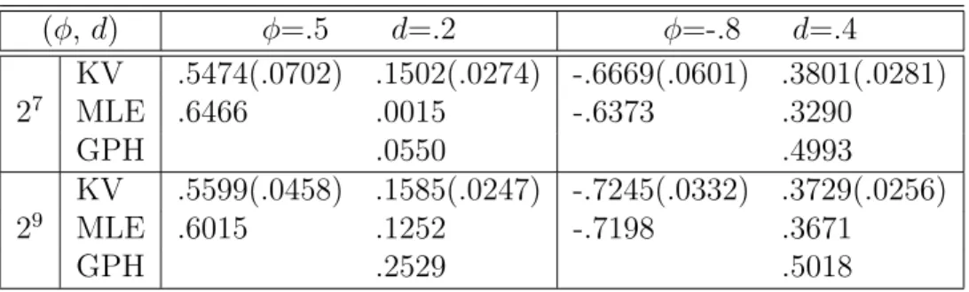
Table 1: ARFIMA(1, d,0): Estimates ofdandφfrom wavelet-based Bayesian method with MP(7) wavelets, MLE and the Geweke and Porter-Hudak (1983) method, re-spectively. Numbers in parentheses are standard errors.
(φ,d) φ=.5 d=.2 φ=-.8 d=.4 KV .5474(.0702) .1502(.0274) -.6669(.0601) .3801(.0281) 27 MLE .6466 .0015 -.6373 .3290 GPH .0550 .4993 KV .5599(.0458) .1585(.0247) -.7245(.0332) .3729(.0256) 29 MLE .6015 .1252 -.7198 .3671 GPH .2529 .5018 4.4 Simulation study
There are a number of ways to generate a time series that exhibits long-memory properties. A computationally simple one was proposed by McLeod and Hipel (1978) and involves the Cholesky decomposition of the correlation matrixRX(i,j) = [ρ(|i−j|)]. Given RX =M M0 with M = [mi,j] a lower triangular matrix, if t, t = 1, . . . , n is a
Gaussian white noise series with zero mean and unit variance, then the series Xt =γ01/2
t
X
i=1 mt,i
will have the autocorrelationρ(τ). The data for Simulation are here generated by us-ing the McLeod and Hipel’s method withσ2 = 1. Simulations to estimate the autore-gressive, moving average parameters and the long memory parameter are performed for ARFIMA(1, d,0), ARFIMA(0, d,1) and ARFIMA(1, d,1) models. For checking robustness of the estimates the simulations are carried out according to different val-ues of parameters (φ = .5,−.8, θ = .5,−.8 and d = .2, .4) and of the sample size n= 27,29. The wavelet family which are used in all simulations is Daubechies (1992) minimum phase wavelets MP(7).
The similar settings to those of Pai and Ravishanker (1996) are used. For each combination of the parameters the estimates based on ten parallel MCMC chains