State space reparametrization for approximating nonlinear models in Bayesian state estimation

(1)

State Space Reparametrization

For Approximating Nonlinear

Models In Bayesian State

Estimation

Jos´

e Luis Franco Monsalve

A Thesis Submitted for the Degree of

Doctor of Philosophy in Electrical Engineering

February 2017

The copyright in this thesis is owned by the author. Any quotation from the thesis or use of any of the information contained in it must acknowledge this thesis as the source of

(2)

Abstract

Recursive Bayesian state estimation is a powerful methodology which is useful for the integration of data about a process of interest while considering all the sources of uncertainty which are present in the observations and in modeling inaccuracies. However, in its general form it is intractable and approximations need to be made in order to use it in real life applications. The most widely used algorithm to perform recursive state estimation is the Kalman filter, which assumes that the probability distributions that it propagates are Gaussian and that the measurement and dy-namical processes are linear. If these assumptions are satisfied, the Kalman filter is optimal. In most applications, however, this proves to be an oversimplification, due to which several techniques have arisen to handle model non-linearity and different types of distributions.

In this thesis, a novel method for the estimation of distributions with nonlinear dynamical and measurement models is presented, which uses a reparametrization of the state space of the distributions in order to exploit the linear properties of the Kalman filter. This involves the mapping of the distribution into a different space, and a subsequent approximation as a Gaussian distribution. An analysis of the adequacy of this transformation is presented, which shows that it is a valid approach in a number of practically interesting filtering problems.

The proposed approach is applied to the estimation of the state of Earth-orbiting objects, as it is a challenging estimation scenario which can benefit from the use of filter. Space situational awareness is increasingly important as near-Earth space becomes cluttered with satellites and debris. In this work, the sensors that are most commonly used to track objects in orbit, radars and telescopes, are modeled and a filter based on the previously discussed ideas is proposed.

Finally, a multi-object estimation filter based on a recent estimation framework is presented which propagates high amounts of information while maintaining low computational complexity. This is important as there are many challenges to track-ing large amounts of orbittrack-ing objects in a principled way ustrack-ing ground-based sensors, and naturally extends the single object filter described above to the multi-sensor, multi-object case.

(3)

List of Figures

2.1 SLR measurements . . . 25

2.2 Data residuals . . . 26

2.3 Estimated measurement likelihood. . . 27

2.4 Kalman filter results . . . 27

2.5 Results of the particle filter on pass 540. . . 29

2.6 Results of the particle filter on pass 737. . . 30

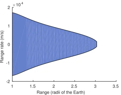
3.1 Typical angular rates admissible region.. . . 48

3.2 Typical range – range rate admissible region. . . 50

3.3 Flowchart for the filtering algorithm with global correction . . . 57

3.4 State extraction . . . 58

3.5 Results of first sensibility experiment . . . 61

3.6 Results of second sensibility experiment. . . 62

3.7 Orbits used for performance evaluation . . . 63

3.8 Estimated covariance (1) . . . 64

3.9 Estimated covariance (2) . . . 65

3.10 RMSE for radar experiment . . . 67

3.11 Radar estimation error and estimated covariance (1). . . 68

3.13 RMSE for optical experiment . . . 70

(7)

4.1 Sample observation paths . . . 79

4.2 Amount of observations in the simulation . . . 90

4.3 Simulated scenario . . . 92

4.4 HISP cardinality estimate . . . 94

4.5 Estimated tracks for object 1 . . . 96

4.6 Position and velocity RMSE for object 1 . . . 97

4.7 Estimated tracks for object 12 . . . 98

4.8 Position and velocity RMSE for object 12 . . . 99

4.9 HISP run time . . . 100

(8)

List of Algorithms

3.1 Track initialization algorithm using radar measurements . . . 48

3.2 Track initialization algorithm using optical measurements . . . 51

3.3 Prediction algorithm . . . 55

3.4 Update algorithm . . . 56

(9)

List of Tables

3.1 Orbital elements of the simulated objects . . . 62 4.1 Sensor resolution and field of view profile . . . 90 4.2 Simulated orbits. . . 91

(10)

Acknowledgments

Producing this PhD. thesis has been the fruit of a large effort, which I would not have been able to manage without the help of many others. I am grateful to my family for their support in setting me on this journey, and to the people who have inspired me to be curious, whether by teaching or by example. I am indebted to the European Commission for the Vibot Erasmus Mundus scholarship without which I would surely not have started this PhD., and to the University and UDRC for providing me with the financial support which enabled me to carry it out.

I have had the fortune to work with very talented people. Thanks to Daniel for being a very engaged supervisor, and leading a team with such high standards of research; It was due to his trust in me that I decided to start this program. Thanks to Manu and J´er´emie for setting an example of hard work, rigor and brilliance which have been an inspiration throughout, and to my fellow students and collaborators for their engagement in producing very high quality work.

I am tremendously fortunate to have met an incredible group of friends in Ed-inburgh, and I am very thankful to them for having made my stay in this city a pleasure. I cannot mention everyone here, but I want to give special thanks to some of them. Thanks to Liam for being contagiously curious and positive, to Shailendra for the good times in so many pubs in Edinburgh, to Peter for the music and for the clever conversations, to Nico for reminding me to take a step back every now and then and breathe. Thanks to Gena, Sarthak and Manu for being not only great friends but also very talented brewing partners, to Corina for being such a good flatmate, to Jos´e for all the good times, to Pablo for showing me so many opportu-nities and pushing me to go after them. Thanks to Alexey for the great times, so many discoveries, and for the time he spent proofreading this work. And thanks to Selma for so much warmth, for all the support, and for being such an inspiration.

(11)

— A riddle, sir? Ask me, sir. — O, ask me, sir.

— A hard one, sir.

— This is the riddle, Stephen said:

The cock crew, The sky was blue: The bells in heaven Were striking eleven. ’Tis time for this poor soul To go to heaven.

What is that? — What, sir?

— Again, sir. We didn’t hear.

Their eyes grew bigger as the lines were repeated. After a silence Cochrane said:

— What is it, sir? We give it up. Stephen, his throat itching, answered:

— The fox burying his grandmother under a hollybush.

Ulysses James Joyce

(12)

Chapter 1 Introduction

S

tatisticalstate estimation is an area of great interest to the engineering

com-munity. With the advent of machines that needed to be controlled based on their state, a reliable means of estimating said state was required in order to take appropriate control actions. The scope of state estimation, however, goes far beyond control applications. Indeed, it is an essential tool in disciplines such as defense, fi-nance, robotics and many more, as it provides a reliable way of handling uncertainty in problems where measurements can not be assumed to give perfect information on the observed system.

The need to estimate the state of increasingly complex systems, coupled with the rapidly expanding availability of low-cost, powerful computer hardware, has spurred the development of estimation algorithms of growing sophistication. The advent of the Kalman filter in the sixties was essential for the success of the Apollo missions, as it permitted to offset the navigation errors with a continual stream of measurements from their on-board sensors [30]. More recently, sophisticated particle filtering algo-rithms have been fundamental for the development of autonomous vehicles whether in air, on the ground, or underwater [94].

Using probability distributions rather than point estimates gives a considerably large amount of information which can be used when decisions need to be taken based on knowledge about the estimated process. Faithfully representing uncertainty in a diversity of domains, however, is a challenging task due to the variety of dynamical and measurement models that arise from different application areas. Filtering tech-niques such as the Kalman filter [47] have proved to be useful in situations where distributions can be reasonably represented with a Gaussian approximation, and the modeled systems are simple enough to be represented with linear transformations. They also benefit from not requiring a large amount of computational resources,

(13)

since they use lean representations for the probability distributions. In more com-plex systems, however, these approximations can result in undesirable effects such as biased distributions, over or underconfident estimations of the uncertainty, and more. More complex filters will naturally require more computational resources to overcome these problems.

A central subject in this thesis is the combination of linear and nonlinear tech-niques in order to minimize the additional resource requirements while still faithfully propagating the distributions. This will usually be carried out by reparametrizing the distributions in order to apply linear operations to the distributions, circum-venting the problems associated with nonlinear dynamical or observation models.

Although estimating the state of single targets has been widely studied, a more general problem is estimating the state of populations of objects, where both the number of targets and their states are unknown [5]. This problem is not as straight-forward as running a number of single target filters in parallel, as it is also necessary to keep in mind the presence of false alarms, where spurious measurements not due to any object of interest in the population appear in the collected data; missed detec-tions, as the probability of detecting individuals in the scene may be less than unity; and data association, as it is necessary to evaluate which measurement correspond to which object in the scene.

Classical approaches to multiple object estimation are based on heuristic exten-sions to single target filters, where data association techniques based on statistical distance are used to hypothesize possible assignments from measurements to tracks, misdetections, or false alarms. Although these approaches are widely used, the heuristics that are used for track management introduce the need for parameter tuning and make it impossible to verify the validity of the filters, e.g. by providing convergence results. A more recent formulation for multiple object state estimation, called finite set statistics [58], is based on the concept of propagating probability distributions based on random sets rather than on random vectors, which has pro-duced principled filters without the previously mentioned limitations of the classical approach. Due to the set representation, however, track identity is not directly propagated between time steps.

A new approach for estimatingstochastic populations [37] has been recently con-ceived which attempts to combine the best aspects of both classical approaches, where track identity is preserved, and finite set statistics, which provides a prin-cipled, extensible framework. Based on the concept of distinguishability, this very recent approach has already produced filters which outperform their state-of-the-art equivalents, especially in scenarios with particularly low probabilities of detection,

(14)

while remaining fully probabilistic in the sense that they do not require the use of heuristics at any stage of the filtering process.

Using principled multi-object state estimation filters has the advantage that since they represent multi-object probability distributions, it is simple to manipulate them in order to create more complex estimation systems. For instance, sensor calibration or localization can be achieved by modeling the joint sensor-population distribution as a hierarchical point process. Multi-sensor fusion can be done through successive updates on the probability distribution using different sensors, and target classification can be done by using multi-model state representations.

This work is principally motivated by the increasing need to have a clear picture of near-Earth space, as the relevance of space-based infrastructure is essential for areas like communications, localization, and defense, among others, and their safety is endangered by the growing amounts of debris residing in orbit. Orbiting objects are typically observed using ground-based sensors such as radars and telescopes, and catalogs of their state is maintained by several agencies. The main available catalogs, however, do not include measures of uncertainty in their estimates, which is essential to evaluating important quantities such as the risk of collision for important assets, or the imprecision in measurements obtained from satellite-mounted sensors that is induced by the uncertainty in their position.

The final goal of this thesis is to present a method which provides a fully proba-bilistic view of near-Earth space, based on noisy measurements from ground based sensors, and which is able to adapt to observing previously undetected objects or sensor clutter. In order to do this, several aspects of estimation for orbital objects will need to be studied. A way to estimate the probability distribution of newly measured objects based on observations that do not include their full state will need to be proposed – telescopes, for instance, cannot measure the distance to an object from Earth and thus cannot resolve its full position. Also, it will be necessary to analyze the dynamics of orbiting objects and how they can be cast in a probabilis-tic framework, alongside modeling ground-based sensors and the uncertainty that they introduce. Finally, a suitable multi-object estimation framework will need to be implemented in order to manage different tracks and give individual informa-tion about observed objects in the presence of data associainforma-tion ambiguity, missed detections and false alarms.

In this context, several important challenges arise. The dynamics of orbiting objects are known with a high degree of accuracy, meaning that there is very low uncertainty in the dynamical models, complicating the use of Monte Carlo methods to propagate distributions. At the same time, their non-linearity makes it

(15)

challeng-ing to use Kalman filter-like algorithms for estimation. In this work, a method which attempts to use the best of both filtering paradigms will be proposed to tackle this problem. In terms of the estimation of populations, it is desirable to have an efficient method which scales well with the number of targets, as the amount of objects to track in orbit is very large.

In this thesis, the previously mentioned filtering principles are illustrated in this domain, and it is shown how they can be used to robustly and efficiently estimate the state of orbiting objects alongside their uncertainty, and maintain a catalog which takes into account the shortcomings of the sensors and the incomplete knowledge of object dynamics.

This manuscript is divided as follows. In Chapter 2, the background of Bayesian estimation and space situational awareness are discussed. Chapter 3 describes a single-object filter for estimating the state of objects in orbit, and Chapter4extends this to the multi-object case using a novel filtering method. Chapter 5 concludes the thesis. Appendix A describes statistical tests for multivariate normality, and Appendix??provides an application to estimation from video data which motivates the reparametrization approach presented in this thesis.

(16)

1.1 Objectives

The objectives of this thesis are the following:

• Present the Bayesian framework for state estimation, alongside commonly used filters that are derived from it, for single and multiple objects.

• Introduce a method to exploit linear filtering techniques in non-linear problems by reparametrizing the state distribution into the sensor space.

• Show a new algorithm for estimating the state of objects in orbit, from data obtained through radio-frequency and electro-optical sensors.

• Extend the previous algorithm to track multiple objects in orbit using a novel multiple object estimation framework.

1.2 Contributions

During the course of this PhD project, the following publications have been produced with contributions from the author, with a note about the level of involvement in the particular work:

• J. Franco, J. Houssineau, D. E. Clark, and C. Rickman. Simultaneous tracking of multiple particles and sensor position estimation in fluorescence microscopy images. In Control, Automation and Information Sciences (ICCAIS), 2013 International Conference on, pages 122–127. IEEE, 2013 — Principal author.

• J. Franco, E. D. Delande, C. Frueh, J. Houssineau, and D. E. Clark. A spherical co-ordinate space parameterisation for orbit estimation. In Proceedings of the 2016 IEEE Aerospace Conference, pages 1–12, 2016 — Principal author, this is the basis for Chapter 3.

• J. Franco, E. D. Delande, C. Frueh, J. Joussineau, and D. Clark. Probabilistic orbit determination using a sensor co-ordinate parametrization. Journal of Guidance, Control and Dynamics, —(—), Under review — Principal author, expands upon the previous publication.

• C. S. Lee, J. Franco, J. Houssineau, and D. E. Clark. Accelerating the single cluster PHD filter with a GPU implementation. In Control, Automation and Information Sciences (ICCAIS), 2014 International Conference on, pages 53– 58. IEEE, Dec 2014 — Experiments.

(17)

1.2 Contributions

• I. Schlangen, J. Franco, J. Houssineau, W. T. E. Pitkeathly, D. E. Clark, I. Smal, and C. Rickman. Marker-less stage drift correction in super-resolution microscopy using the single-cluster PHD filter. IEEE Journal of Selected Top-ics in Signal Processing, 10(1):193–202, 2016 — Concept, writing, part of the experiments.

• J. Houssineau, D. E. Clark, S. Ivekovic, C. S. Lee, and J. Franco. A unified ap-proach for multi-object triangulation, tracking and camera calibration. IEEE Transactions on Signal Processing, 64(11):2934–2948, 2016 — Experiments, validation of the distributions. This publication inspired the development of the methods shown in Chapter 3.

• O. Hagen, J. Houssineau, I. Schlangen, E. D. Delande, J. Franco, and D. E. Clark. Joint estimation of telescope drift and space object tracking. In

Aerospace Conference, 2016 IEEE, pages 1–10. IEEE, 2016 — Support with the basic algorithm that was used in the application.

• C. Simpson, A. Hunter, S. Vorgul, E. D. Delande, J. Franco, and D. E. Clark. Likelihood modelling of the space geodesy facility laser ranging sensor for Bayesian filtering. In Sensor Signal Processing for Defence (SSPD), 2016, pages 1–5. IEEE, 2016 — Concept, writing, supervision of the students. Case study in Chapter 2.

• A. Pak, J. Correa, M. Adams, D. E. Clark, E. D. Delande, J. Houssineau, J. Franco, and C. Frueh. Joint target detection and tracking filter for Chilbolton advanced meteorological radar data processing. InAdvanced Maui Optical and Space Surveillance Technologies Conference, 2016 — Support with basic con-cepts.

• E. D. Delande, J. Houssineau, J. Franco, C. Frueh, and D. E. Clark. A new multi-target tracking algorithm for a large number of orbiting objects. In

Proceedings of the 27th AAS/AIAA Space Flight Mechanics Meeting, San An-tonio, TX, 2017 — Implementation, integration of SSA models, experiments, writing. Forms the basis for Chapter 4.

• E. D. Delande, C. Frueh, J. Franco, J. Houssineau, and D. E. Clark. A novel multi-object filtering approach for space situational awareness. Journal of Guidance, Control, and Dynamics, 2017. submitted — Integration of SSA models, experiments.

(18)

1.2 Contributions

The research project which the author was part of involved work from many collaborators. The particular contributions of the author were the following:

Chapter 2 Performed literature review. Supervised students in the development of range-tracking filter for Herstmonceux laser ranging facility.

Chapter 3 Developed probabilistic initial orbit determination method for radar and optical sensors. Collaborated in the creation of a radar tracking filter and developed the optical filter. Validated the distributions using Henze-Zirkler tests. Performed experiments and wrote two articles based on the work in this chapter.

Chapter 4 Implementation and integration of SSA models into the HISP filter. Experiments and validation.

(19)

Chapter 2 Background

T

hischapter covers probabilistic state estimation from a Bayesian point of view;

that is, the integration of observation data from a process of interest with models about how this data is generated and how the process behaves in order to produce probability distributions that describe its state. This is framed in the con-text of Space Situational Awareness (SSA), as it will be the main application focus for this thesis. First, an overview of techniques used for estimation in space situa-tional awareness will be presented, followed by a detailed description of the general Bayesian filtering paradigm. After this, commonly used filters for the estimation of the state of single objects will be presented, after which a review of state estimation methods for populations of objects where not only the number of objects in the pop-ulation must be estimated, but also their individual states, will be made. Finally, methods which extend these estimation methods in order to additionally estimate parameters of the observed process will be described. This will give an overview of the state of the art of state estimation, which will set the stage for the contributions of the thesis in later chapters.

2.1 Estimation in space situational awareness

Space infrastructure plays an increasingly important part in modern communica-tions, reconnaissance, and geolocation, among other applicacommunica-tions, and as more na-tions increase their stake in the exploitation of near-Earth space the number of artificial satellite launches increases year after year. Each of these launches gener-ates debris which endangers current and future missions, and in spite of mitigation efforts this remains a very relevant problem. Safeguarding orbital assets, then, involves knowing their position and velocity with a high degree of accuracy and

(20)

pre-2.1 Estimation in space situational awareness

cision, and also any potential collision risks that could be posed by other satellites or by space debris [49].

Using noisy data to estimate the state of objects in orbit can be accomplished in several ways. For instance, when a fixed amount of data is available to estimate the parameters of an object, nonlinear curve fitting algorithms can be used [32]. Ap-plications for this include the estimation of orbital parameters in remote planetary sensing applications [92]. In this thesis, the recursive Bayesian estimation paradigm is employed to estimate the state of orbiting objects as it enables the integration of data as it comes, giving instantaneous information about the uncertainty of the orbital estimate. This is particularly valuable when unknown objects appear in orbit, or there are sudden perturbations which change the state of known objects. Additionally, it enables the implementation of tractable multi-object estimation al-gorithms as data association only needs to be performed from a time step to the next rather than over all available data in past time instants.

Since the very beginning, the Kalman filter and its extensions have been in-valuable in the domain of space situational awareness. From its use to plan and execute the Apollo moon missions [30] to global navigation systems such as GPS [31], passing by orbit determination and re-entry estimation methods [43], it has been indispensable in most developments which have enabled humankind to explore space.

Although techniques to propagate orbits from a known initial state have been widely studied, the problem of estimating the collision risk of two objects naturally benefits from knowing what the uncertainty of its position and velocity are. A prob-lem with using only deterministic propagation to predict the position of an object is that the object may drift away from its initially estimated orbit due to pertur-bations such as space weather effects. Additionally, if an object is only observed once, unique orbit determination is not possible as only a subset of the full state is observable [95]. With this in mind, filtering algorithms such as the Kalman filter and its extensions attempt to propagate probability distributions rather than only a point estimate, and to use incoming measurements to decrease the uncertainty of the estimated orbit [8].

The most commonly used sensors used for space situational awareness are radar and optical sensors [76], although other sensors can be used such as laser ranging systems [86]. Radars are commonly used to track objects in space, and combined measurements typically give information about the azimuth and elevation of the object, its distance to the station, and the rate of change of this distance when Doppler information is available. Combined optical measurements are obtained from

(21)

2.1 Estimation in space situational awareness

telescopes, and give azimuth, elevation, and their rates of change. While telescopes can see objects that are very far away, they rely on passive illumination by the sun and clear weather conditions; whereas although radars have the advantage of using active sensing, it is costly to see objects that are far since radar energy returns are inversely proportional to the fourth power of the distance [76].

When the initial state of an object that is being observed is not known, it can be recovered deterministically if three measurements from the same target are avail-able using Gauss’ method, double R iteration [21] or Gooding’s method [27]. This is prone to errors due to measurement noise, however, and requires a reliable method to determine that the measurements come from the same target. A recent develop-ment in orbit determination has produced the admissible regions approach, which offers constraints on the possible states of a target given that a single measurement is available [95]. In the Bayesian context, it is possible to use these energy con-straints to generate a prior distribution based on a single measurement. This will be elaborated in chapter 3.

A limitation of the Kalman filter and its nonlinear extensions is that it relies on linearization of the orbital dynamics and observation models to produce its esti-mates, which will fail if the estimate uncertainty is too large causing the linearization to lose validity [45]. This is particularly the case for the distributions of objects that have been observed only once, as the range of values, and thus the uncertainty, of the unobserved parameters is very large [95].

Classical approaches to solve the statistical orbit determination problem rely on the Extended Kalman Filter [8] and its variants, which can only represent Gaussian distributions, and thus the banana-shaped uncertainties that are found in orbital estimation problems cannot be represented by it. This problem has been recognized by the community, and solutions based on Gaussian sum filters have been proposed instead, which are more flexible in the representation of the distribution [93, 96]. Another issue is that the measurement models are highly nonlinear so important information can be lost through their linearization; and as it was shown in [45], it gives biased estimates for range-bearing style problems as is the case in orbit determination. For this reason, the Unscented Kalman Filter [45] has been explored in orbital estimation situations. It relies on the propagation of the first two moments of the filtering distribution, which are however insufficient to represent arbitrary priors.

The bootstrap filter [29] is commonly used in problems where the dynamical or measurement models are nonlinear, and allows for modeling of arbitrarily shaped dis-tributions. The performance of particle filtering with respect to classical approaches

(22)

2.2 Bayesian filtering

has been demonstrated in [60], and hybrid approaches which also use a UKF when measurements are available have also been explored to reduce the uncertainty when measurements are acquired [70]. Another way of representing uncertainty, based on generalized polynomial chaos, is able to model parametric uncertainty in addition to perturbations and uncertain initial conditions [51].

Several approaches have been used in the past to track multiple objects in space. The MHT [87], Labeled Multi-Bernoulli [44] or CPHD [44] filters are examples of this. Although these take into account the problems that arise in multiple object estimation, they also suffer from several shortcomings – random finite set approaches discard track identities, or try to propagate them in inefficient ways. Classical approaches are heuristic based and it is not possible to theoretically verify that their population management techniques are correct. The advantages and shortcomings of these methods will be described in section2.5. The stochastic populations framework [14,37] has been recently proposed to both maintain track identities while remaining a theoretically principled method, and it will be described in detail later in the chapter.

The remainder of this chapter describes the recursive Bayesian state estimation framework, which will be exploited in subsequent chapters to derive single- and multi-object filters for space situational awareness.

2.2 Bayesian filtering

Filtering is the process through which the probabilistic estimate, or filtering distri-bution, of the object state is maintained as time passes, by using the dynamical model of the object; and corrected when data is acquired, by using a model of how the sensor observes the object [5]. These models also take into account the uncer-tainties induced by the sources mentioned above. If these models are available, then the filtering distribution can be obtained by applying the following recursion:

pk|k−1(x|z1:k−1) = Z fk(x|x0)pk−1(x0|z1:k−1) dx0 (2.1) pk(x|z1:k) = gk(zk|x)pk|k−1(x|z1:k−1) R gk(zk|x0)pk|k−1(x0|z1:k−1) dx0 , (2.2)

where pk|k−1(x|z1:k−1) is the predicted density at time k; fk(x|x0) is the nonlinear

state transition kernel of the system, i.e., the probability of the target being in state

(23)

2.2 Bayesian filtering

to time k; and gk(zk|x) is the measurement model, or the likelihood of observing

measurementzk conditioned on statex. The explicit conditioning on the past

mea-surements will be dropped from here onwards for reasons of succinctness. Equation (2.1) is called the Chapman-Kolmogorov equation, and uses the knowledge about how the process evolves in time to predict the filtering distribution before receiving any additional data. Equation (2.2) is an application of Bayes’ rule, and uses the measurement model to integrate the information of any acquired measurements into the filtering distribution. It is clear that further to this, a prior distribution p0(x)

is required in order to recursively compute the subsequent distributions. This dis-tribution represents any available knowledge about the object state before starting the filtering process, and proper modeling of this initial distribution is essential to obtaining accurate results. All together, this recursion is called the Bayes filter [80], and does not constrain the form of the estimated distributions or the used models. The evolution of the process of interest through time is considered through the dynamical model. The function fk(x|x0) summarizes the knowledge of how the

state of the target evolves through time, and models also any uncertainty on this evolution. Dynamical models range from Brownian motion, where the only source of movement is random; passing by constant velocity or constant acceleration mod-els, where it is assumed that these vector quantities only vary due to unmodeled sources; to sophisticated models for maneuvering targets. A survey of commonly used dynamical models can be found in [75], emphasizing those used for maneuver-ing targets where it is critical to properly model their motion. In certain cases, the dynamics of the objects that are modeled are very well known. One such case is that of orbital objects, in which case the dynamical models can be borrowed from the physical models describing their motion [7]. This case is studied further in Chapter 3.

The measurement model gk(zk|x) describes the type of measurements that are

acquired by the sensor, conditioned on the object state and possibly other measured properties such as its attitude or reflectivity, and the sensor’s own measurement capabilities at the time of the observation. Although the measurements will be used to refine the estimate of the state of the object, it is possible that the sensor can only observe part of the state of interest such that it is not possible to fully resolve it using a single measurement. Additionally, the measurement model takes into account its noise characteristics, in order to incorporate this source of uncertainty into the filtering process. Measurement models can be anything from a fully observed process, to complex non-linear interactions between the observed process and the sensor. In further chapters, measurement models for different filtering problems are

(24)

2.3 Single object state estimation

presented, including a way to model the sensor induced uncertainty.

2.3 Single object state estimation

Although (2.1) and (2.2) describe the statistically optimal filter for arbitrary forms of the filtering distributions, in practice computing the integrals becomes intractable unless the functional forms of the probability distributions is constrained. These equations do not have closed form solutions in most cases, a notable exception being that of Gaussian functions. In this section, the most commonly used approaches to tractably use the Bayes filter are presented, starting with the closed form solutions in the Kalman filter family of methods, followed by numerical integration approaches. The purpose of showing this variety of single object state estimation filters is that not only do they provide the essential building blocks to multiple object state estimation algorithms, but also that according to the application, some filters will be more suitable than others. In further chapters, new filters are derived that are based on the ones described below, which makes it important to introduce them here.

2.3.1 Closed form solutions

The Kalman filter is one of the most widely used solutions to the tractable imple-mentation of the Bayes filter [47]. It propagates the mean and covariance of the distribution of the observed process under certain conditions; namely, that the mea-surement and dynamical models are linear and their respective random terms are zero mean uncorrelated Gaussian random variables:

fk(xk|xk−1) =Fxk−1+t, t ∼ N(·; 0, Qk); (2.3) gk(zk|xk) =Hxk+νk, νk ∼ N(·; 0, Rk), (2.4) where N(x;µ,Σ) = (2π)−d2|Σ|− 1 2 e− 1 2(x−µ) 0_Σ−1₍_x₋_µ₎ (2.5) is a multivariate Gaussian distribution with mean µ, covariance Σ, evaluated at

d-dimensional point x; and F and H are the matrices dictating the linear trans-formations of the dynamical and measurement processes, respectively. If this is the case, the Kalman filter uses the prior mean and covariance of the process µk−1 and

(25)

Pk−1 to obtain in first instance the predicted mean and covariance

µk|k−1 =Fµk−1 (2.6)

Pk|k−1 =F Pk−1F0+Qk. (2.7)

From here, when a measurement is obtained, it becomes possible to compute the innovation mean zk − Hµk|k−1 and its covariance S = HPk|k−1H0 +Rk, which

describe the distribution of the difference between the observed measurement with respect to the expected measurement. This permits the computation of the and the

Kalman gain K = Pk|k−1H0S−1, which minimizes the variance of the estimator of

the updated mean and covariance

µk =µk|k−1+K(zk−Hµk|k−1) (2.8)

Pk = (I−KH)Pk|k−1. (2.9)

Kalman’s original article on this filter tackles the problem from a signal processing point of view, but it is also interesting to consider the problem from a Bayesian statistics point of view, as analyzed by Ho and Lee in [36]. In here, it is shown that if the prior distribution is Gaussian, not only can these statistics be obtained but the complete form of the distribution can be analytically determined to be Gaussian with the parameters shown above. This is because under a Gaussian likelihood, Gaussian functions are conjugate priors with themselves [69].

The main advantages of the Kalman filter are that it is not only robust and principled, but also readily implementable and computationally efficient. However, the requirement that the measurement and dynamical models be linear turns out to be too restrictive for a wide class of problems, which turn out to include space situational awareness, as both the dynamical and measurement models are non-linear [8].

The attractive properties of the Kalman filter, coupled with the urgent need to filter nonlinear systems that was spurred by the need to localize the Apollo spacecraft as it made its way to the moon [30] led to the development of the Extended Kalman filter (EKF) (See e.g. [5]). Rather than requiring linear transformations represented by matrices, general dynamical and measurement models are used:

fk(xk|xk−1) = f(xk−1) +t, t∼ N(·; 0, Qk); (2.10) gk(zk|xk) = h(xk) +νk, νk∼ N(·; 0, Rk). (2.11)

(26)

Here, the functionsf andg are required to be differentiable as the extended Kalman filter relies on the linearization of these models obtained from their first-order Taylor expansions. It can be noted here that more general functions of the formf(xk−1,t)

andh(xk,νk) can be used, but only the simpler case with additive noise is illustrated

here for simplicity. The function f is linearized with respect to its parameter to obtain the matrix

Fk = ∂f ∂xk−1 xk−1=µk−1 . (2.12)

The mean of the predicted distribution is computed by applying the full state tran-sition function to the prior mean, but the covariance is obtained using the linearized function:

µk|k−1 =f(µk−1) (2.13)

Pk|k−1 =FkPk−1Fk0 +Qk. (2.14)

Having obtained this, the measurement model is also linearized around the predicted mean to obtain Hk = ∂g ∂xk xk=µk|k−1 . (2.15)

Similarly, the innovationzk−h(µk|k−1) is computed with the full nonlinear function,

while the innovation covariance and Kalman gain are calculated with the linear approximation: Sk =HkPk|k−1Hk0 +Rk andKk =Pk|k−1Hk0S

−1

k . This is sufficient to

obtain the updated mean and covariance of the distribution:

µk=µk|k−1+K(zk−g(µk|k−1)) (2.16)

Pk= (I−KH)Pk|k−1. (2.17)

It must be stressed that while under the assumptions outlined above the Kalman filter yields distributions that are statistically optimal, the linearization in the EKF causes the resulting distributions to be only approximate. The degree to which the models can be linearized will determine how accurate the obtained filtering distributions will be.

A more recent development in Kalman-like filters is the Unscented Kalman Filter (UKF) [46]. The key idea of this method is that rather than approximating the functions that compose the dynamical and measurement models, it is simpler and more effective to approximate the distribution using a fixed number of samples. The filter proceeds by decomposing the prior into a set of sigma points and associated

(27)

weights, in such a way that the resulting empirical distribution will have the same statistics as the original distribution; then propagating these points through the full nonlinear functions; and finally using the resulting points to compute the statistics required to obtain the filtering distribution. This approach differs from particle filtering techniques in that the set of sigma points is chosen in a deterministic way, and the weights do not indicate probabilities.

To use the prior to obtain a set of sigma points, the state must be extended to include the noise terms in the transition kernel fk(xk|xk−1) = f(xk−1,k), by

ex-tending the mean and covariance of the distribution with those ofk. A common way

to obtain these points is to use the Cholesky decomposition of its covariance matrix to obtain a set of points which have the same statistics µk−1 and Pk−1. If the i-th

column of the Cholesky decomposition of Pk−1 is denoted σi, it is straightforward

to verify that the distribution of 2N + 1 points

x0_k₋₁ =µk−1

x(_ki₋)₁ =µk−1+σi, i= 1,2, . . . , N

x(_kN₋+₁i)=µk−1−σi, i= 1,2, . . . , N,

(2.18)

whereN is the dimension of the extended state, has the desired mean and covariance. The predicted mean and covariance are then obtained by propagating these sigma points through the transition kernel and computing the statistics:

µk|k−1 = 1 2N + 1 2N+1 X i=0 f(x(_ki₋)₁), (2.19) Pk|k−1 = 1 2N + 1 2N X i=0 (f(x(_ki₋)₁)−µk|k−1)(f(x (i) k−1−µk|k−1) 0 , (2.20)

wheref acts on the extended state vector instead of the original state vector and the random term. To obtain the updated term, these are extended with the observation noise term νk in the measurement model gk(zk|xk) = h(xk,νk). Following the

process outlined above, the extended covariance is again decomposed to obtain the 2M+ 1 predicted sigma points x(_ki₊₁) _|_k and the predicted observation ˆzk is obtained:

ˆ zk = 1 2M + 1 2M X i=0 h(x(_ki₊₁) _|_k), (2.21)

with M the dimension of the extended state space. The expected observation is then used alongside the sigma points to obtain the innovation covarianceS, and the

(28)

2.3 Single object state estimation state-observation cross-correlation Pxz: S = 1 2M + 1 2M X i=0 (h(x(_ki₊₁) _|_k)−zˆk) (2.22) Pxz = 1 2M + 1 2M X i=0 (x(_ki₊₁) _|_k−µk|k−1)(h(x (i) k+1|k)−zˆk) 0 . (2.23)

From this, the Kalman gain can be computed as

K =PkzS−1, (2.24)

from which the updated mean and covariance can be obtained:

µk =µk|k−1+K(z−zˆk) (2.25)

Pk =Pk|k−1−KSK0. (2.26)

An advantage of using filters in this family have to do with the fact that since the full dynamical and measurement models are used rather than approximations, certain biases can be eliminated. In particular, linearizing the commonly used trans-formation between polar and Cartesian co-ordinates has been shown to yield biased results in the EKF, which does not happen in the UKF [45]. Additionally, deriving and programming the Jacobian matrices required in the EKF is not necessary, which is an intensive and error-prone process.

If priors which can be reasonably represented with a mean and a covariance can be used, the UKF is an attractive method as it is simple and computationally efficient. However, it can be difficult to apply this method if the distributions that are used cannot be represented like this, as is the case in the priors presented in chapter 3.

Since the methods shown above represent distributions through a mean and a covariance, they cannot appropriately propagate multimodal distributions. Even if a distribution is unimodal, the performance of the filter will suffer when the shape of the distribution does not resemble that of a Gaussian. In order to solve these problems, the Gaussian sum filter was proposed, which is based on the observation that it is possible to use Gaussian mixtures to approximate a wide range of distri-butions [1, 88]. Gaussian sum filters represent the filtering distribution as a sum of

(29)

weighted Gaussian distributions:

pk(x|z1:k) = N X

i=1

w_k(i)N(x;µ_k(i), P_k(i)). (2.27)

Prediction is applied to each individual Gaussian term in the same way as the previously mentioned filters, and weights are left unchanged. For update, the update operation of the above-described filters is also applied to each individual Gaussian, after which the weights are updated based on the individual innovation and its covariance: w(_ki₊₁) = w (i) k N(z−h(µ (i) k|k+1); 0, S (i) k ) PN j=1w (j) k N(z−h(µ (j) k|k+1); 0, S (j) k ) . (2.28)

A big advantage of closed-form solutions is that the parameters of the posterior distribution can be found even if the mismatch between the prior distribution and the measurement likelihood always exists. This is in contrast to numerical methods, where Gaussians are essentially truncated after a certain distance from the mean, such that the product of two Gaussians can numerically be zero even if it is not the case theoretically. Unfortunately, this comes with the imprecision that is added by the involved approximations.

2.3.2 Numerical integration

In cases where the state space of the variable to estimate is sufficiently small, the integrals in (2.1) and (2.2) can be solved numerically. If the state space is discrete, these can be calculated for each possible state, and the filter is called the discrete Bayes filter. If it is hybrid or continuous, it is first discretized into bins, and a representative point in each of these bins is used for prediction and update. This method is called the histogram filter [94].

Since it is common for some regions of the state space to concentrate lower cu-mulative probability than others, the state space can be decomposed unevenly to represent the regions with higher likelihood with greater granularity, while using a more compact representation for regions that don’t accumulate a lot of probability. For this, methods such as quad- or oct-trees can be used [94]. Another interesting method is that of optimal stochastic quantization, which learns a discrete represen-tation of the state space which has higher resolution in the higher likelihood regions [4].

The main disadvantage of solving Bayes’ filter numerically is that as the volume and dimension of the state space increases, the problem becomes increasingly

(30)

un-2.3 Single object state estimation

tractable from the computational point of view. This issue, usually called the curse of dimensionality, has motivated the development of Monte Carlo methods which are more tractable in high-dimensional state spaces.

2.3.3 Monte Carlo methods

An alternative to parametric filters such as the ones described above is the family of Monte Carlo methods. These algorithms rely on solving the intractable integrals which determine the predicted and updated state distributions using Monte Carlo integration, which consists on making use of a weighted sample representation of the probability distribution of the object state, and then using the weighted samples to approximate the continuous integral as a discrete sum. This is useful since if it is possible to drawN samples{x(_ki)}N

i=1 from a distribution of interest, it is possible to

estimate expected values using the following approximation [18]:

Epk(f) = Z f(x)pk(x)dx≈ 1 N N X i=1 f(x(_ki)), (2.29)

where Epk(f) denotes the expected value of functionf under probability distribution

pk.

Representing a distribution with samples is not only useful to compute expected values (from where the statistics of the distribution can be obtained), but also to get an idea of the shape of the distribution, as areas with higher concentration of particles integrate to higher probability. Equation (2.29) assumes that it is possible to obtain independent, identically distributed (IID) samples from the probability distribution pk. Generally, however, obtaining samples from arbitrary distributions

is not straightforward. The importance sampling framework is commonly used to overcome this difficulty. It is based on the principle that the above expectation is equivalent to

Epk(f) =

Z

pk(x)

π(x)f(x)π(x)dx, (2.30)

whereπ, called the importance sampling function, is a probability distribution which can be easily sampled from, with support overlapping that ofpk. This suggests that

(31)

2.3 Single object state estimation equation (2.29) to obtain Epk(f)≈ N X i=1 w(_ki)f(x(_ki)), with (2.31) w_k(i) = pk(x (i) k )/π(x (i) k ) PN j=1pk(x (j) k )/π(x (j) k ) . (2.32)

An alternative way of seeing this is that the probability distribution is being approximated with a set ofweighted samples{x(_ki), w(_ki)}N

i=1, with higher weights

rep-resenting higher likelihood for each particular sample. As the importance sampling function is used to obtain samples to represent the updated distribution, the filter efficiency will improve if these two distributions are close. If it is possible to di-rectly sample from the updated distribution (2.2), e.g., if pk−1|k−1(x) is Gaussian

and gk(zk|x) and f(x|x0) are linear and Gaussian and methods such as the ones

described in section 2.3.1 are used, then the proposal is said to be optimal as it minimizes the variance of the importance weights [18].

To maintain a representative sample of the distribution, resampling is usually performed which replaces low weighted particles by particles in areas of higher like-lihood, thus increasing the resolution of the distribution in the regions where more precision is required. This is done by replacing the weighted sample {x˜(_ki), w_k(i)}N

i=1

by an equally weighted sample {x(_ki),_N1}N

i=1, with probability Pr(x (i) k = ˜x (j) k ) = w (j) k .

These two sets of particles approximate the same original distribution.

In order to obtain samples from the distribution, methods such as those in the Markov chain Monte Carlo (MCMC) family can be used. For example, the Metropolis-Hastings algorithm requires only a conditional proposal distribution q

and a function that is proportional to the probability distribution to sample from,

f(x)∝p(x) [34]. The fact that the probability distribution only needs to be known up to a constant of proportionality is useful in this case as it means that the denomi-nator in (2.2) does not need to be computed, for instance. The method approximates the distributionp(·) by starting at an initial random sample x0 and iteratively

sam-pling from a proposal kernel conditioned on the current point, ˜xk ∼q(·|xk−1). This

is accepted as the next sample xk = ˜xk if p(˜xk) ≥ p(xk−1). If the probability is

lower, then it is accepted with probabilityf(˜xk)/f(xx−1) and rejected otherwise, in

which case xk = xk−1. Since this method tends to generate autocorrelated chains,

and needs to generate a number of samples before it achieves the desired stationary distribution, it requires the generation of a number of samples before converging to it, in addition to the usual requirement ofthinning, or only taking one sample every

(32)

N samples generated from the obtained sequence, in order to avoid these undesired correlations.

The MCMC family of methods rely on exploring regions of the state space with high probabilities, as they need to provide more samples in these regions than in oth-ers. Simple Brownian motion can be used as a proposal kernel in a process known as Random Walk Monte Carlo, but the process will be aided by using more information about the target distribution such as its gradient, as this enables the exploration of higher likelihood areas. Methods that exploit this include the Metropolis Adjusted Langevin Algorithms (MALA), which uses Langevin dynamics which make use of the gradient of the logarithm of the posterior to create a stochastic sequence that converges to this distribution [74]. Hamiltonian Monte Carlo, in turn, uses Hamil-tonian dynamics to explore the state space [62]. This involves using an auxiliary momentum variable, and has also been shown to perform very well.

In cases where it is simple to sample from sub-groups of variables of the target distribution, and it is possible to compute the conditional distributions of the re-mainder of the variables on this sub-group, Gibbs sampling may be used [9]. This is an effective way of reducing the dimensionality of the problem, which greatly reduces the complexity of MCMC methods.

More methods exist to obtain samples from the desired distribution, including deterministic surrogate and optimization-based methods. An extensive survey of stochastic simulation methods such as these can be found in [65].

As the time step k in (2.1) and (2.2) increases, generating samples using these methods becomes increasingly onerous as the complete chain of samples must be generated from the beginning up to the current time step. Sequential Monte Carlo methods, however, allow for the computation of the current filtering distribution conditioned on the previous belief, which is ideally suited to the filtering problem as only one sample needs to be generated instead of having to recompute the entire particle trajectory [18]. This filter is initialized with a sample of the prior distribu-tion, {x(₀i) ∼ p0(·)}Ni=1, with equal weights w

(i)

0 = 1/N, i = 1,· · · , N. At time step

k, when a measurement zk is received, it obtains the samples

x(_ki)∼f(·|x(_ki₋)₁) followed by the importance weights

w_k(i) = w˜ (i) k PN i=1w˜ (i) k , w˜(_ki)=g(zk|x (i) k )w (i) k−1,

(33)

2.4 Case study: A filter for laser ranging

which is followed by resampling to avoid particle degeneracy. As it can be seen, the classical bootstrap filter [29] uses the Markov transition kernel for each particle as an importance function, but does not use any information about the received measurement. Proposal distributions which make use of the measurement are called

fully adapted, and will naturally approximate the desired distribution better as they use all the available information up to the current time step.

A way to use a fully adopted proposal in the particle filtering framework is to use a MCMC rejection method to approximate the optimal distribution when sampling the next particle [41]. The advantage of this approach is that the optimal proposal is approximated directly, minimizing the variance of the particle weights. With this, however, comes a highly increased computational cost. An alternative to this is the Auxiliary Particle Filter [66]. In here, an additional step is performed to randomly select a particle from the previous time step such that samples of higher likelihood are obtained, and integrates the measurement likelihood into the proposal distribution. This additional step yields more particles in the more informative regions of the state space. After this, the proposal weights are computed as before. This filter has been shown to strike a balance between computational efficiency and filter performance. The issues involved with using particle filters in SSA have to do with the fact that samples are needed from the Bayes filter recursion. The transition kernel tends to be very narrow, as very little noise is needed in dynamical models for orbiting objects. This is usually problematic in Monte Carlo approaches and tends to be solved by using bridging densities [18]. These are intermediate densities which converge at a given rate to the desired density. The problem with this is that the computational cost of the resulting algorithm is greatly increased due to the intermediate sampling steps.

2.4 Case study: A filter for laser ranging

In this section, single object filtering is illustrated by applying it to data acquired from a ground-based laser ranging station that measures the distance from it to satellites equipped with retroreflectors. The output of the range-only laser sensor at the Herstmonceux Space Geodesy Facility is analysed in order to design a sensor Section2.4uses material from ‘Likelihood modelling of the Space Geodesy Facility laser ranging sensor for Bayesian filtering’ [86], C. Simpson, A. Hunter, S. Vorgul, E. Delande, J. Franco, D. Clark, published in the proceedings of the Sensor Signal Processing for Defence (SSPD) conference, used with permission. c2016 IEEE.

(34)

model for filtering purposes. The sensor model is then exploited for the design of a single-target Bayesian filter, comparing a Kalman filter and a particle filter.

The Space Geodesy Facility in Herstmonceux (East Sussex, UK) is a multi-technique geodetic observatory operating an SLR station, an absolute gravimeter and several Global Navigation Satellite System (GNSS) receivers. Along with forty other similar sites around the world, the SGF in Herstmonceux forms part of the International Laser Ranging Service (ILRS) [64]. The SLR technique, used primar-ily for geodetic purposes, measures the time of flight of short laser pulses as they travel between the observing stations and orbiting satellites equipped with retrore-flectors [10,83]. Satellites routinely tracked by the ILRS network include low Earth orbiters with scientific payloads (e.g. Grace, Jason-3, Swarm), passive geodetic tar-gets (e.g. LAGEOS, LARES), and various GNSS constellations (e.g. GLONASS, BeiDou, GPS). Capable of providing measurements with sub-centimeter accuracy and precision, SLR is one of the four space geodetic techniques contributing to the realization of the International Terrestrial Reference Frame [2]. Beyond geodetic applications, SLR can also be employed to track uncooperative space debris objects (i.e. no retroreflectors present) [50, 102].

An Nd:Van pulsed laser (1 KHz repetition rate, 10 ps FWHM pulse width, 1.1 mJ/pulse) at the frequency-doubled wavelength of 532 nm is employed at the SGF laser station. The receiver telescope is a 0.5 m Cassegrain reflector equipped with a Single Photon Avalanche Diode (SPAD) detector. The timing measurements are provided by a home built event timer of 1 ps resolution and 5 ps precision. A strictly single-photon tracking policy is followed at SGF for all satellite targets, whereby the energy levels of the returned pulses are controlled and limited to ensure that, on av-erage, only a single photon is contained in each reflected pulse. This ensures that the laser retroreflector arrays carried onboard the satellite targets are sampled in their entirety, with no preferential detections obtained from points closer to the ground station. In order to limit the negative impact of background and dark noise events, the detector is gated shortly earlier (typically 100 ns) than the predicted range to the satellite. This is necessary due to the high sensitivity of the sensor and the present background radiation. The distribution of returns, excluding actual satellite reflections, are adequately described with a negative exponential distribution, as the detection events follow Poisson statistics [83]. The specific characteristics of the distribution of detected pulses from the satellite targets depend on the shape and orientation of the laser retroreflector arrays.

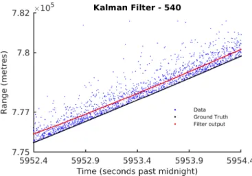
Three datasets collected from the SGF laser, named 746, 540, 737 for different satellite passes, can be seen in Figure 2.1. The identities of the observed satellites

(35)

is known, and the ground truth, shown in the figure is obtained from an avail-able catalog. These figures illustrate the typical features of the raw ranging data collected at SGF, though they all present a very noticeable skewness in the data distribution around the ground truth. The data residuals are depicted in Figure2.2. In particular, batch 737 has an atypical shape in the lower range values due to a temporal problem in the receiver hardware caused by laser overlap, which happens when a pulse is fired at the same time a detector is gated. The pulse backscatters off the atmosphere and triggers the detector. This run was recorded when the overlap avoidance routine was disabled.

2.4.1 Filter design

A simple constant velocity motion model will be used to track the position and velocity of each object. The state will be denoted xt = (r,r˙), and its dynamics are

modeled as xt= " 1 ∆t 0 1 # xt−1 +nt, (2.33)

with nt ∼ N(0, Qt) is the process noise vector. The measurement model is more

interesting, as it is evident from the residuals in Figure2.2that the noise distribution does not have a Gaussian form. In order to obtain a suitable likelihood function, an exponential curve was fit to the residuals of batch 746, obtaining the following estimated relation:

`(zt|xt)∝exp(−2.811×10−4(zt−rt)). (2.34)

The resulting curve can be seen in Figure 2.3.

In order to implement a Kalman filter, a Gaussian distribution was fit to the residuals of the same batch in order to produce a linear observation model. The results of this filter can be seen in Figure 2.4. From this figure, it can be seen that since the filter expects a symmetrical distribution for the measurement noise, it produces biased estimates.

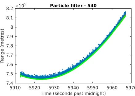
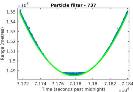
A simple bootstrap filter was also implemented, as described in Section 2.3.3. The filter was applied to datasets 540 and 737, using the likelihood function esti-mated from dataset 746. As it can be seen in Figure2.1, batch 540 has a very similar noise distribution to the training set while batch 737 has some artifacts resulting in a more complicated noise structure. The results of applying the filter with dataset 540 can be seen in Figure 2.5, where it can be seen how the effects of the noisy

(36)

(a) Batch 746

(b) Batch 540

(c) Batch 737

(37)

(a) Batch 746

(b) Batch 540

(c) Batch 737

(38)

2.4 Case study: A filter for laser ranging Range difference(metres)

0 2000

4000

6000

8000

Probability density

0

1

2

3

4

Histogram Fit

Figure 2.3: Estimated measurement likelihood

(39)

2.5 Multiple object state estimation

measurements are reasonably filtered out. Figure 2.6 shows the results of the filter on batch 737. Here, it can be seen that the filter is also robust to sudden changes in the distribution of the noise.

This sample filtering application shows how it is possible to handle different noise profiles by adequately modeling the measurement likelihood functions, and how Kalman filtering is not always applicable. The results indicate that the estimates are consistent with the object states found in the catalog, in spite of the challenging noise profile.

2.5 Multiple object state estimation

Multiple object estimation, or multi-target tracking, is the problem of simultane-ously estimating the state of a group of objects of interest as it evolves through time, and its unknown and time-varying size. This is particularly interesting as it is general enough to study multiple problems of interest, including disciplines such as simultaneous localization and mapping (robotics) [53], biological microscopy [25], and defense [58]. Estimating the state of such a system, however, is rarely as easy as estimating the states of each one of its components, due to a multiple of problems which include the uncertainty of track-to-measurement associations, the possible presence of spurious measurements in the data which are not produced by any ob-ject of interest, and the possibility of missed detections, all of which increase the difficulty of the estimation process [5].

Several approaches to solve the multi-object estimation problem exist, which can be broadly divided into three categories. The first category can be referred to as the ‘classical’ category, and attempts to use heuristics based on data association techniques to assign measurements to single-object filters. The second category is made up of filters based on Finite Set Statistics (FISST), which attempt to track the whole population by estimating probability densities defined onrandom sets rather than random vectors. The third category is based on a new formulation based on the concept of distinguishability in stochastic processes. These techniques will be described below.

2.5.1 Classical approaches

Classical methods of multi-target tracking are based on heuristic systems that man-age a group of single target filters, assigning them measurements according to data association heuristics. The Joint Probabilistic Data Association Filter (JPDAF)

(40)

(a) Maxima and minima of the filtering distribution throughout the estimation (green), measurements (blue)

(b) Detail of filtering results. Measurements and extrema as above, ground truth (orange), estimate (red).

(41)

(a) Maxima and minima of the filtering distribution throughout the estimation (green), measurements (blue)

(b) Detail of filtering results. Measurements and extrema as above, ground truth (orange), estimate (red).

(42)

assumes that the number of targets is known, and assign measurements as either being produced by a particular track or being a false alarm, leaving the remainder of the tracks as tracks with a missed detection [5]. The data association mechanism is based on the Mahalanobis distance between tracks and measurements. The clear disadvantage of this technique is that the number of tracks must be known before-hand by the operator, and is assumed to remain constant during the estimation process - In many applications, target appearance and disappearance are essential components of the dynamics of the multi-object system.

The Multiple Hypothesis Tracking (MHT) filter [71] is one of the most com-monly used target tracking filters today, perhaps due to the fact that it is a rather straightforward extension of single-target filtering techniques. It incorporates tar-get appearance and disappearance into the filtering process by considering, for each measurement, whether it was originated by either one of the previous tracks, a false alarm, or a new track.

Each group of associations where each measurement is assigned to one of these categories is called a hypothesis, and single target filters are run to evaluate the new multi-target state per hypothesis. The likelihood of each hypothesis is then evaluated by combining the individual filter likelihoods, and taking into account the likelihood of the hypothesized false alarms and misdetections. Further heuristics help curb the geometric growth of hypotheses, which would make the algorithm prohibitively expensive to run after some time. Although this approach considers the necessary components to make a useful multi-target tracker, the extensive use of heuristics adds to the problem the need of tuning a number of additional parameters and makes it hard to validate the filter analytically (e.g., by providing convergence results).

It is worth noting here that different domain-specific methods exist for tracking which have not been mentioned here. For instance, active contour methods such as the one described in [48] can be used to effectively track moving objects in images based on edge motion, or acoustic trackers such as those based on iterative time reversal techniques are used to interactively focus energy on targets of interest with active sonar systems [68]. The focus of this thesis, however, is to analyze general tracking methodologies rather than these domain-specific methods.

2.5.2 Random finite set solutions

Finite Set Statistics (FISST) is an approach which generalizes the single-object Bayes filter to multiple targets by using random finite sets (RFS) rather than

State space reparametrization for approximating nonlinear models in Bayesian state estimation