Discovering Latent Network
Structure in Point Process Data
The Harvard community has made this
article openly available.
Please share
how
this access benefits you. Your story matters
Citation
Linderman, Scott, and Ryan P. Adams. 2014. "Discovering Latent
Network Structure in Point Process Data." In Proceedings of The
31st International Conference on Machine Learning, Beijing, China,
June 22-24, 2014. Journal of Machine Learning Research: W&CP 32:
1413–1421.
Published Version
http://jmlr.org/proceedings/papers/v32/linderman14.pdf
Citable link
http://nrs.harvard.edu/urn-3:HUL.InstRepos:17491847
Terms of Use
This article was downloaded from Harvard University’s DASH
repository, and is made available under the terms and conditions
applicable to Open Access Policy Articles, as set forth at
http://
nrs.harvard.edu/urn-3:HUL.InstRepos:dash.current.terms-of-use#OAP
Scott W. Linderman [email protected]
Harvard University, Cambridge, MA 02138 USA
Ryan P. Adams [email protected]
Harvard University, Cambridge, MA 02138 USA
Abstract
Networks play a central role in modern data anal-ysis, enabling us to reason about systems by studying the relationships between their parts. Most often in network analysis, the edges are given. However, in many systems it is diffi-cult or impossible to measure the network di-rectly. Examples of latent networks include eco-nomic interactions linking financial instruments and patterns of reciprocity in gang violence. In these cases, we are limited to noisy observations of events associated with each node. To enable analysis of these implicit networks, we develop a probabilistic model that combines mutually-exciting point processes with random graph mod-els. We show how the Poisson superposition principle enables an elegant auxiliary variable formulation and a fully-Bayesian, parallel infer-ence algorithm. We evaluate this new model em-pirically on several datasets.
1. Introduction
Many types of modern data are characterized via relation-ships on a network. Social network analysis is the most commonly considered example, where the properties of in-dividuals (vertices) can be inferred from “friendship” type connections (edges). Such analyses are also critical to un-derstanding regulatory biological pathways, trade relation-ships between nations, and propagation of disease. The tasks associated with such data may be unsupervised (e.g., identifying low-dimensional representations of edges or vertices) or supervised (e.g., predicting unobserved links in the graph). Traditionally, network analysis has focused onexplicit network problems in which the graph itself is considered to be the observed data. That is, the vertices
Proceedings of the 31st International Conference on Machine Learning, Beijing, China, 2014. JMLR: W&CP volume 32. Copy-right 2014 by the author(s).
are considered known and the data are the entries in the as-sociated adjacency matrix. A rich literature has arisen in recent years for applying statistical machine learning mod-els to this type of problem, e.g.,Liben-Nowell & Kleinberg (2007);Hoff(2008);Goldenberg et al.(2010).
In this paper we are concerned withimplicit networksthat cannot be observed directly, but about which we wish to perform analysis. In an implicit network, the vertices or edges of the graph may not be directly observed, but the graph structure may be inferred from noisy emissions. These noisy observations are assumed to have been gen-erated according to underlying dynamics that respect the latent network structure.
For example, trades on financial stock markets are executed thousands of times per second. Trades of one stock are likely to cause subsequent activity on stocks in related in-dustries. How can we infer such interactions and disen-tangle them from market-wide fluctuations? Discovering latent structure underlying financial markets not only re-veals interpretable patterns of interaction, but also provides insight into the stability of the market. In Section4we will analyze the stability of mutually-excitatory systems, and in Section6we will explore how stock similarity may be in-ferred from trading activity.
As another example, both the edges and vertices may be latent. In Section 7, we examine patterns of violence in Chicago, which can often be attributed to social structures in the form of gangs. We would expect that attacks from one gang onto another might induce cascades of violence, but the vertices (gang identity of both perpetrator and vic-tim) are unobserved. As with the financial data, it should be possible to exploit dynamics to infer these social struc-tures. In this case spatial information is available as well, which can help inform latent vertex identities.
In both of these examples, the noisy emissions have the form of events in time, or “spikes,” and our intuition is that a spike at a vertex will induce activity at adjacent ver-tices. In this paper, we formalize this idea into a
probabilis-tic model based on mutually-interacting point processes. Specifically, we combine the Hawkes process (Hawkes, 1971) with recently developed exchangeable random graph priors. This combination allows us to reason about latent networks in terms of the way that they regulate interaction in the Hawkes process. Inference in the resulting model can be done with Markov chain Monte Carlo, and an elegant data augmentation scheme results in efficient parallelism.
2. Preliminaries
2.1. Poisson ProcessesPoint processes are fundamental statistical objects that yield random finite sets of events{sn}N
n=1⊂ S, whereS
is a compact subset of RD, for example, space or
time. The Poisson process is the canonical exam-ple. It is governed by a nonnegative “rate” or “inten-sity” function, λ(s) :S →R+. The number of events
in a subset S0⊂ S follows a Poisson distribution with meanR
S0λ(s)ds. Moreover, the number of events in
dis-joint subsets are independent. We use the notation{sn}N
n=1∼ PP(λ(s))to indicate that
a set of events {sn}N
n=1 is drawn from a Poisson process
with rateλ(s). The likelihood is given by p({sn}Nn=1|λ(s)) = exp − Z S λ(s)ds N Y n=1 λ(sn). (1)
In this work we will make use of a special property of Pois-son processes, the Poisson superposition theorem, which states that {sn} ∼ PP(λ1(s) +. . .+λK(s))can be de-composed into K independent Poisson processes. Let-ting zn denote the origin of the n-th event, we perform the decomposition by independently sampling each zn from Pr(zn=k)∝λk(sn), fork∈ {1. . . K} (Daley & Vere-Jones,1988).
2.2. Hawkes Processes
Though Poisson processes have many nice properties, they cannot capture interactions between events. For this we turn to a more general model known as Hawkes pro-cesses (Hawkes,1971). A Hawkes process consists ofK point processes and gives rise to sets of marked events {sn, cn}Nn=1, wherecn ∈ {1, . . . , K}specifies the process on which the n-th event occurred. For now, we assume the events are points in time, i.e., sn∈[0, T]. Each of the K processes is a conditionally Poisson process with a rateλk(t| {sn:sn < t})that depends on the history of events up to timet.
Hawkes processes have additive interactions. Each process has a “background rate”λ0,k(t), and each eventsnon pro-cesskadds a nonnegative impulse responsehk,k0(t−sn)
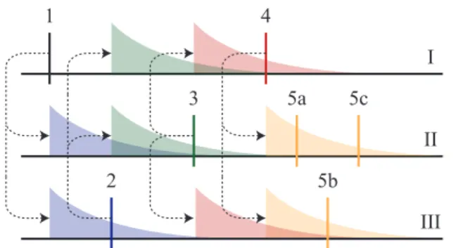
1 2 3 4 5a 5b 5c I II III Figure 1: Illustration of a Hawkes process. Events induce impulse responses on connected processes and spawn “child” events. See the main text for a complete description.
to the intensity of other processesk0. Causality and locality of influence are enforced by requiringhk,k0(∆t)to be zero
for∆t /∈[0,∆tmax].
By the superposition theorem for Poisson processes, these additive components can be considered independent pro-cesses, each giving rise to their own events. We augment our data with a latent random variablezn ∈ {0, . . . , n−1} to indicate the cause of then-th event (0if the event is due to the background rate and1. . . n−1if it was caused by a preceding event). The augmented Hawkes likelihood is then the product of likelihoods of each Poisson process:
p({(sn, cn, zn)}Nn=1| {λ0,k(t)},{{hk,k0(∆t)}}) = K Y k=1 p({sn :cn =k∧zn = 0} |λ0,k(t))× N Y n=1 K Y k=1 p({sn0 :cn0 =k∧zn0 =n} |hc n,k(t−sn)),
where the densities in the product are given by Equation1. Figure1illustrates a causal cascades of events for a simple network of three processes (I-III). The first event is caused by the background rate (z1= 0), and it induces impulse
responses on processes II and III. Event 2 is spawned by the impulse on the third process (z2= 1), and feeds back
onto processes I and II. In some cases a single parent event induces multiple children, e.g., event 4 spawns events 5a-c. In this simple example, processes excite one another, but do not excite themselves. Next we will introduce more sophisticated models for such interaction networks.
2.3. Random Graph Models
Graphs of K nodes correspond to K×K matrices. Unweighted graphs are binary adjacency matrices A whereAk,k0 = 1indicates a directed edge from nodekto
nodek0. Weighted directed graphs can be represented by a real matrixW whose entries indicate the weights of the edges. Random graph models reflect the probability of
dif-ferent network structures through distributions over these matrices.
Recently, many random graph models have been unified under an elegant theoretical framework due to Aldous and Hoover (Aldous, 1981; Hoover, 1979). See Lloyd et al. (2012) for an overview. Conceptually, the Aldous-Hoover representation characterizes the class ofexchangeable ran-dom graphs, that is, graph models for which the joint probability is invariant under permutations of the node la-bels. Just as de Finetti’s theorem equates exchangeable se-quences to independent draws from a random probability measure , Aldous-Hoover renders the entries ofA condi-tionally independent given latent variables of each node. Empty graph models (Ak,k0 ≡0) and complete
mod-els (Ak,k0 ≡1) are trivial examples, but much more
structure may be encoded. For example, consider a model in which nodes are endowed with a location in space,xk ∈RD. This could be an abstract feature space
or a real location like the center of a gang territory. The probability of connection between two notes decreases with distance between them asAk,k0 ∼Bern(ρe−||xk−xk0||/τ),
whereρis the overall sparsity andτ is the characteristic distance scale. This is known as alatent distance model. Many models can be constructed in this manner. Stochastic block models, latent eigenmodels, and their nonparametric extensions all fall under this class (Lloyd et al.,2012). We will leverage the generality of the Aldous-Hoover formal-ism to build a flexible model and inference algorithm for Hawkes processes with structured interaction networks.
3. The Network Hawkes Model
In order to combine Hawkes processes and random net-work models, we decompose the Hawkes impulse response hk,k0(∆t)as follows:
hk,k0(∆t) =Ak,k0Wk,k0gθ
k,k0(∆t). (2) Here, A∈ {0,1}K×K is a binary adjacency matrix and W ∈RK×K
+ is a non-negative weight matrix.
To-gether these specify thesparsity structureandstrength of the interaction network, respectively. The non-negative functiongθk,k0(∆t)captures the temporal aspect of the
in-teraction. It is parameterized by θk,k0 and satisfies two
properties: a) it has bounded support for∆t∈[0,∆tmax],
and b) it integrates to one. In other words,gis a probability density with compact support.
Decomposinghas in Equation2has many advantages. It allows us to express our separate beliefs about the spar-sity structure of the interaction network and the strength of the interactions through a spike-and-slab prior on A andW (Mohamed et al.,2012). The empty graph model recovers independent background processes, and the
com-plete graph recovers the standard Hawkes process. Mak-ingg a probability density endowsW with units of “ex-pected number of events” and allows us to compare the relative strength of interactions. The form suggests an intuitive generative model: for each impulse response drawm∼Poisson(Wk,k0)number of induced events and
draw themchild event times i.i.d. fromg, enabling com-putationally tractable conjugate priors.
Intuitively, the background rates, λ0,k(t), explain events
that cannot be attributed to preceding events. In the sim-plest case the background rate is constant. However, there are often fluctuations in overall intensity that are shared among the processes, and not reflective of process-to-process interaction, as we will see in the daily variations in trading volume on the S&P100 and the seasonal trends in homicide. To capture these shared background fluctua-tions, we use a sparse log Gaussian Cox process (Møller et al.,1998) to model the background rate:
λ0,k(t) =µk+αkexp{y(t)}, y(t)∼ GP(0, K(t, t0)).
The kernel K(t, t0) describes the covariance structure of the background rate that is shared by all processes. For ex-ample, a periodic kernel may capture seasonal or daily fluc-tuations. The offsetµk accounts for varying background intensities among processes, and the scaling factorαk gov-erns how sensitive processkis to these background fluctu-ations (whenαk = 0we recover the constant background rate).
Finally, in some cases the process identities,cn, must also be inferred. With gang incidents in Chicago we may have only a location,xn ∈R2. In this case, we may place a
spa-tial Gaussian mixture model over thecn’s, as inCho et al. (2013). Alternatively, we may be given the label of the community in which the incident occurred, but we suspect that interactions occur between clusters of communities. In this case we can use a simple clustering model or a non-parametric model like that ofBlundell et al.(2012).
3.1. Inference with Gibbs Sampling
We present a Gibbs sampling procedure for inferring the model parameters,W,A,{{θk,k0}},{λ0,k(t)}, and, if
nec-essary, {cn}. In order to simplify our Gibbs updates, we will also sample a set of parent assignments for each event{zn}. Incorporating these parent variables enables conjugate prior distributions forW,θk,k0, and, in the case
of constant background rates,λ0,k. Detailed derivations are
provided in the supplementary material.
Sampling weights W. A gamma prior on the weights, Wk,k0 ∼Gamma(α0W, βW0 ), results in the conditional
dis-tribution, Wk,k0| {sn, cn, zn}Nn=1, θk,k0∼Gamma(αk,k0, βk,k0), αk,k0 =αW0 + N X n=1 N X n0=1 δcn,kδcn0,k0δzn0,n βk,k0 =βW0 + N X n=1 δcn,k.
The posterior parameters correspond to the number of events caused by an interaction and the total unweighted rate induced by events on nodek. Here and elsewhere,δi,j is the Kronecker delta function. We use the inverse-scale parameterization of the gamma distribution .
Sampling background rates λ0,k. Similarly, for background rates λ0,k(t)≡λ0,k, the prior
λ0,k∼Gamma(α0λ, β
0
λ) is conjugate with the likeli-hood and yields the conditional distribution
λ0,k| {sn, cn, zn}Nn=1,∼Gamma(αλ, βλ), αλ=α0λ+ X n δcn,kδzn,0 βλ=β0λ+T
This conjugacy no longer holds for log Gaussian Cox pro-cess background rates, but conditioned upon the parent variables, we must simply fit a log Gaussian Cox process for those events for whichzn= 0. We use elliptical slice sampling (Murray et al.,2010) for this purpose.
Sampling impulse response parameters θk,k0. The
logistic-normal density with parameters θk,k0 = {µ, τ}
provides a flexible model for the impulse response: gk,k0(∆t|µ, τ) = 1 Z exp ( −τ 2 σ−1 ∆t ∆tmax −µ 2) σ−1(x) = ln(x/(1−x)) Z =∆t(∆tmax−∆t) ∆tmax τ 2π −12 . The normal-gamma priorµ, τ ∼ N G(µ, τ|µ0
µ, κ0µ, α0τ, βτ0) is conjugate and results in a conditional distribution with the following sufficient statistics:
xn,n0 = ln(sn0−sn)−ln(tmax−(sn0 −sn)), m= N X n=1 N X n0=1 δcn,kδcn0,k0δzn0,n, ¯ x= 1 m N X n=1 N X n0=1 δcn,kδcn0,k0δz n0,nxn,n0.
Intuitively, these correspond to the number of events caused by an interaction and their average delay.
Collapsed Gibbs sampling A and zn. With Aldous-Hoover graph priors, the entries in the binary adjacency matrixAare conditionally independent given the param-eters of the prior. The likelihood introduces dependencies between the rows ofA, but each column can be sampled in parallel. Gibbs updates are complicated by strong de-pendencies between the graph and the parent variables,zn. Specifically, if zn0 =n, then we must haveAc
n,cn0 = 1. To improve the mixing of our sampling algorithm, first we updateA| {sn, cn},W, θk,k0 by marginalizing the parent
variables. The posterior is determined by the likelihood of the conditionally Poisson processλk0(t| {sn:sn < t})
(Equation 1) with and without interaction Ak,k0 and the
prior comes from the Aldous-Hoover graph model. Then we updatezn| {sn, cn},A,W, θk,k0 by sampling from the
discrete conditional distribution. Though there areN par-ent variables, they are conditionally independpar-ent and may be sampled in parallel. We have implemented our inference algorithm on GPUs to capitalize on this parallelism.
Sampling process identitiescn. As with the adjacency matrix, we use a collapsed Gibbs sampler to marginalize out the parent variables when sampling the process identi-ties. Unfortunately, thecn’s are not conditionally indepen-dent and hence must be sampled sequentially.
Computational concerns. Compact impulse responses limit the number of potential event parents and significantly reduce the memory requirements and running time of our algorithm. If the average firing rate is constant, the ex-pected number of potential parents per event will be linear inK. Summing the per-event contributions to the log like-lihood can be done inO(logN)time using standard paral-lel reductions. Hence, after paralparal-lelizing over the columns ofAand the parentszn, one step of our sampling algorithm takesO(K(K+ logN))time when process identities are known, andO((K+N)(K+ logN))time otherwise. On the datasets used in the following experiments, our GPU implementation1achieves 5-50 iterations per second.
4. Stability of Network Hawkes Processes
Due to their recurrent nature, Hawkes processes must be constrained to ensure their positive feedback does not lead to infinite numbers of events. A stable system must satisfy2
λmax= max |eig(AW)|<1
(c.f.Daley & Vere-Jones(1988)). When we are condition-ing on finite datasets we do not have to worry about this. We simply place weak priors on the network parameters,
1https://github.com/slinderman 2
In this contextλmaxrefers to an eigenvalue rather than a rate,
(a) 0 1 2 0 2 4 6 W p(W) G(1,5) G(2,5) G(4,8) G(8,12) (b) 4 64 1024 10−2 10−1 100 K ρ (c) 0 0.5 1 λ max Pr( λ max ) (d) 0 0.5 1 λ max Pr( λ max )
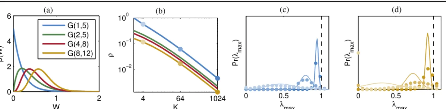
Figure 2: Empirical and theoretical distribution of the maximum eigenvalue for Erd˝os-Renyi graphs with gamma weights. (a) Four gamma weight distributions. The colors correspond to the curves in the remaining panels. (b) Sparsity that theoretically yields99% probability of stability as a function ofp(W)andK. (c) and (d) Theoretical (solid) and empirical (dots) distribution of the maximum eigenvalue. Color corresponds to the weight distribution in (a) and intensity indicatesKandρshown in (b).
e.g., a beta prior on the sparsityρof an Erd˝os-Renyi graph, and a Jeffreys prior on the scale of the gamma weight distri-bution. For the generative model, however, we would like to set our hyperparameters such that the prior distribution places little mass on unstable networks. In order to do so, we use tools from random matrix theory.
The celebrated circular law describes the asymptotic eigen-value distribution for K ×K random matrices with en-tries that are i.i.d. with zero mean and variance σ2.
As K grows, the eigenvalues are uniformly distributed over a disk in the complex plane centered at the origin and with radius σ√K. In our case, however, the mean of the entries,µ=E[Ak,k0Wk,k0], is not zero. Silverstein
(1994) has analyzed such “noncentral” random matrices and shown that the largest eigenvalue is asymptotically dis-tributed asλmax∼ N(µK, σ2).
In the simple case of Wk,k0 ∼Gamma(α, β)
and Ak,k0∼Bern(ρ), we have µ=ρα/β and
σ=pρ((1−ρ)α2+α)/β. For a givenK,αandβ, we
can tune the sparsity parameterρto achieve stability with high probability. We simply setρsuch that the minimum ofσ√Kand, say,µK+ 3σ, equals one. Figures2aand2b show a variety of weight distributions and the maximum stable ρ. Increasing the network size, the mean, or the variance will require a concomitant increase in sparsity. This approach relies on asymptotic eigenvalue distribu-tions, and it is unclear how quickly the spectra of ran-dom matrices will converge to this distribution. To test this, we computed the empirical eigenvalue distribution for random matrices of various size, mean, and variance. We generated 104 random matrices for each weight
distribu-tion in Figure2awith sizesK = 4,64, and1024, andρ set to the theoretical maximum indicated by dots in Fig-ure2b. The theoretical and empirical distributions of the maximum eigenvalue are shown in Figures2cand2d. We find that for small mean and variance weights, for exam-ple Gamma(1,5) in the Figure2c, the empirical results closely match the theory. As the weights grow larger, as in Gamma(8,12) in 2d, the empirical eigenvalue
distri-butions have increased variance and lead to a greater than expected probability of unstable matrices for the range of network sizes tested here. We conclude that networks with strong weights should be counterbalanced by strong spar-sity limits, or additional structure in the adjacency matrix that prohibits excitatory feedback loops.
5. Synthetic Results
Our inference algorithm is first tested on synthetic data gen-erated from the network Hawkes model. We perform two tests: a) a link prediction task where the process identities are given and the goal is to simply infer whether or not an interaction exists, and b) an event prediction task where we measure the probability of held-out event sequences. The network Hawkes model can be used for link predic-tion by considering the posterior probability of interac-tionsP(Ak,k0| {sn, cn}). By thresholding at varying
prob-abilities we compute a ROC curve. A standard Hawkes process assumes a complete set of interactions (Ak,k0 ≡1),
but we can similarly threshold its inferred weight matrix to perform link prediction.
Cross correlation provides a simple alternative measure of interaction. By summing the cross-correlation over off-sets ∆t∈[0,∆tmax), we get a measure of directed
inter-action. A probabilistic alternative is offered by the gen-eralized linear model for point processes (GLM), a pop-ular model for spiking dynamics in computational neuro-science (Paninski, 2004). The GLM allows for constant background rates and both excitatory and inhibitory inter-actions. Impulse responses are modeled with linear ba-sis functions. Area under the impulse response provides a measure of directed excitatory interaction that we use to compute a ROC curve. See the supplementary material for a detailed description of this model.
We sampled ten network Hawkes processes of 30 nodes each with Erd˝os-Renyi graph models, constant background rates, and the priors described in Section3. The Hawkes processes were simulated forT= 1000seconds. We used
0 0.2 0.4 0.6 0.8 1 0 0.2 0.4 0.6 0.8 1 FP rate TP rate
Synthetic Link Prediction ROC
Net. Hawkes Std. Hawkes GLM XCorr
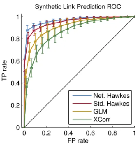
Figure 3: Comparison of models on a link prediction test aver-aged across ten randomly sampled synthetic networks of 30 nodes each. The network Hawkes model with the correct Erd˝os-Renyi graph prior outperforms a standard Hawkes model, GLM, and simple thresholding of the cross-correlation matrix.
1 2 3 4 5 6 7 8 9 10 0 1 2 3 4 5 Network
Pred. log lkhd. (bits/s)
Synthetic Predictive Log Likelihood
Net Hawkes Std Hawkes GLM
Figure 4: Comparison of predictive log likelihoods for the same set of networks as in Figure3, compared to a baseline of a Pois-son process with constant rate. Improvement in predictive likeli-hood over baseline is normalized by the number of events in the test data to obtain units of “bits per spike.” The network Hawkes model outperforms the competitors in all sample networks. the models above to predict the presence or absence of in-teractions. The results of this experiment are shown in the ROC curves of Figure3. The network Hawkes model ac-curately identifies the sparse interactions, outperforming all other models. With the Hawkes process and the GLM we can evaluate the log likelihood of held-out test data. On this task, the network Hawkes outperforms the competitors for all networks. On average, the network Hawkes model Financial Model Pred. log lkhd. (bits/spike)
Indep. LGCP 0.594
Std. Hawkes 0.912
Net. Hawkes (Erd˝os-Renyi) 0.903 Net. Hawkes (Latent Distance) 0.888
Figure 5: Comparison of financial models on a event prediction task, relative to a homogeneous Poisson process baseline.
achieves2.2±.1bits/spike improvement in predictive log likelihood over a homogeneous Poisson process. Figure4 shows that on average the standard Hawkes and the GLM provide only 60% and 72%, respectively, of this predictive power. See the supplementary material for further analysis.
6. Trades on the S&P 100
As an example of how Hawkes processes may discover interpretable latent structure in real-world data, we study the trades on the S&P 100 index collected at 1s intervals during the week of Sep. 28 through Oct. 2, 2009. Every time a stock price changes by ±0.1%of its current price an event is logged on the stock’s process, yielding a total ofK= 100processes andN=182,037 events.
Trading volume varies substantially over the course of the day, with peaks at the opening and closing of the market. This daily variation is incorporated into the background rate via a log Gaussian Cox process (LGCP) with a pe-riodic kernel (see supplementary material). We look for short-term interactions on top of this background rate with time scales of∆tmax= 60s. In Figure5we compare the predictive performance of independent LGCPs, a standard Hawkes process with LGCP background rates, and the
net-τ
Latent Dimension 1
Latent Dimension 2
Inferred Embedding of Financial Stocks
IT Financials Energy Health Care Consumer Industrials
AAPL JNJ JPM CVS PG WAG XOM
Top 4 eigenvectors of A ⋅W
Figure 6: Top: A sample from the posterior distribution over em-beddings of stocks from the six largest sectors of the S&P100 under a latent distance graph model with two latent dimensions. Scale bar: the characteristic length scale of the latent distance model. The latent embedding tends to embed stocks such that they are nearby to, and hence more likely to interact with, others in their sector. Bottom: Hinton diagram of the top 4 eigenvectors. Size indicates magnitude of each stock’s component in the eigen-vector and colors denote sectors as in the top panel, with the addi-tion of Materials (aqua), Utilities (orange), and Telecomm (gray). We show the eigenvectors corresponding to the four largest eigen-valuesλmax= 0.74(top row) toλ4= 0.34(bottom row).
Communities Clusters 0 0.1 0.2 0.3 0.4 Process ID Model
Pred. Log Lkhd (bits/s)
Empty Complete Erdos−Renyi Distance (a) Receiving Cluster Initiating Cluster Cluster Interactions 1 2 3 4 1 2 3 4 0 20 40 (b) −87.9 −87.8 −87.7 −87.6 −87.5 41.6 41.65 41.7 41.75 41.8 41.85 41.9 41.95 42 42.05 42.1
Inferred Gang Regions
Cluster 1 Cluster 2 Cluster 3 Cluster 4 (c) 1980 1985 1990 1994 0 1 2 3 λ1 (t) 1980 1985 1990 1994 0 1 2 3 λ2 (t) 1980 1985 1990 1994 0 1 2 3 λ3 (t) 1980 1985 1990 1994 0 1 2 3 λ4 (t) [Hom/Day/km 2] × 10 −3 Offset Background Interactions (d)
Figure 7: Inferred interactions among clusters of community areas in the city of Chicago. (a) Predictive log likelihood for “communities” and “clusters” process identity models and four graph models. Panels (b-d) present results for the model with the highest predictive log likelihood: an Erd˝os-Renyi graph withK= 4clusters. (b) The weighted interaction network in units of induced homicides over the training period (1980-1993). (c) Inferred clustering of the 77 community areas. (d) The intensity for each cluster, broken down into the offset, the shared background rate, and the interactions (units of10−3homicides per day per square kilometer).
work Hawkes model with LGCP background rates under two graph priors. The models are trained on four days of data and tested on the fifth. Though the network Hawkes is slightly outperformed by the standard Hawkes, the differ-ence is small relative to the performance improvement from considering interactions, and the inferred network parame-ters provide interpretable insight into the market structure. In the latent distance model for A, each stock has a la-tent embeddingxk∈R2such that nearby stocks are more
likely to interact, as described in Section 2.3. Figure 6 shows a sample from the posterior distribution over embed-dings inR2forρ= 0.2andτ= 1. We have plotted stocks
in the six largest sectors, as listed on Bloomberg.com. Some sectors, notably energy and financials, tend to cluster together, indicating an increased probability of interaction between stocks in the same sector. Other sectors, such as consumer goods, are broadly distributed, suggesting that these stocks are less influenced by others in their sector. For the consumer industry, which is driven by slowly vary-ing factors like inventory, this may not be surprisvary-ing. The Hinton diagram in the bottom panel of Figure6shows the top 4 eigenvectors of the interaction network. All eigen-values are less than 1, indicating that the system is stable. The top row corresponds to first eigenvector (λmax= 0.74).
Apple (AAPL), J.P. Morgan (JPM), and Exxon Mobil (XOM) have notably large entries in the eigenvector, suggesting that their activity will spawn cascades of self-excitation.
7. Gangs of Chicago
In our final example, we study spatiotemporal patterns of gang-related homicide in Chicago. Sociologists have sug-gested that gang-related homicide is mediated by under-lying social networks and occurs in mutually-exciting, re-taliatory patterns (Papachristos,2009). This is consistent with a spatiotemporal Hawkes process in which processes correspond to gang territories and homicides incite further homicides in rival territories.
We study gang-related homicides between 1980 and 1995 (Block et al.,2005). Homicides are labeled by the com-munity in which they occurred. Over this time-frame there wereN = 1637gang-related homicides in the77 commu-nities of Chicago.
We evaluate our model with an event-prediction task, train-ing on 1980-1993 and testtrain-ing on 1994-1995. We use a LGCP temporal background rate in all model variations. Our baseline is a single process with a uniform spatial rate for the city. We test two process identity models: a) the “community” model, which considers each community a separate process, and b) the “cluster” model, which groups communities into processes. The number of clusters is cho-sen by cross-validation (see supplementary material). For each process identity model, we compare four graph mod-els: a) independent LGCPs (empty), b) a standard Hawkes process with all possible interactions (complete), c) a
net-work Hawkes model with a sparsity-inducing Erd˝os-Renyi graph prior, and d) a network Hawkes model with a latent distance model that prefers short-range interactions. The community process identity model improves predic-tive performance by accounting for higher rates in South and West Chicago where gangs are deeply entrenched. Al-lowing for interactions between community areas, how-ever, results in a decrease in predictive power due to over-fitting (there is insufficient data to fit all772potential in-teractions). Interestingly, sparse graph priors do not help. They bias the model toward sparser but stronger interac-tions which are not supported by the test data. These re-sults are shown in the “communities” group of Figure7a. Clustering the communities improves predictive perfor-mance for all graph models, as seen in the “clusters” group. Moreover, the clustered models benefit from the inclusion of excitatory interactions, with the highest predictive log likelihoods coming from a four-cluster Erd˝os-Renyi graph model with interactions shown in Figure 7b. Distance-dependent graph priors do not improve predictive perfor-mance on this dataset, suggesting that either interactions do not occur over short distances, or that local rivalries are not substantial enough to be discovered in our dataset. More data is necessary to conclusively say which.
Looking into the inferred clusters in Figure7c and their rates in7d, we can interpret the clusters as “safe suburbs” in gold, “buffer neighborhoods” in green, and “gang ter-ritories” in red and blue. Self-excitation in the blue clus-ter (Figure 7b) suggests that these regions are prone to bursts of activity, as one might expect during a turf-war. This interpretation is supported by reports of “a burst of street-gang violence in 1990 and 1991” in West Englewood (41.77◦N,−87.67◦W) (Block & Block,1993).
Figure7dalso shows a significant increase in the homicide rate between 1989 and 1995, consistent with reports of es-calating gang warfare (Block & Block,1993). In addition to this long-term trend, homicide rates show a pronounced seasonal effect, peaking in the summer and tapering in the winter. A LGCP with a quadratic kernel point-wise added to a periodic kernel captures both effects.
8. Related Work
Gomez-Rodriguez et al.(2010) introduced one of the ear-liest algorithms for discovering latent networks from cas-cades of events. They developed a highly scalable approx-imate inference algorithm, but they did not explore the po-tential of random network models or emphasize the point process nature of the data.Simma & Jordan(2010) studied this problem from the context of Hawkes processes and de-veloped an expectation-maximization inference algorithm. We have adapted their latent variable formulation in our
fully-Bayesian inference algorithm and introduced a frame-work for prior distributions over the latent netframe-work. Others have considered special cases of the model we have proposed. Blundell et al. (2012) combine Hawkes pro-cesses and the Infinite Relational Model (a specific ex-changeable graph model with an Aldous-Hoover represen-tation) to cluster processes and discover interactions. Cho et al.(2013) applied Hawkes processes to gang incidents in Los Angeles. They developed a spatial Gaussian mixture model (GMM) for process identities, but did not explore structured network priors. We experimented with this pro-cess identity model but found that it suffers in predictive log likelihood tests (see supplementary material).
Recently, Iwata et al. (2013) developed a stochastic EM algorithm for Hawkes processes, leveraging similar conju-gacy properties, but without network priors. Zhou et al. (2013) have developed a promising optimization-based ap-proach to discovering low-rank networks in Hawkes pro-cesses, similar to some of the network models we explored. Perry & Wolfe(2013) derived a partial likelihood inference algorithm for Hawkes processes with a similar emphasis on structural patterns in the network of interactions. They provide an estimator capable of discovering homophily and other network effects. Our fully-Bayesian approach gener-alizes this method to capitalize on recent developments in random network models (Lloyd et al.,2012).
Finally, generalized linear models (GLMs) are widely used in computational neuroscience (Paninski,2004). GLMs al-low for both excitatory and inhibitory interactions, but, as we have shown, when the data consists of purely excitatory interactions, Hawkes processes outperform GLMs in link-and event-prediction tests.
9. Conclusion
We developed a framework for discovering latent network structure from spiking data. Our auxiliary variable formu-lation of the multivariate Hawkes process supported arbi-trary Aldous-Hoover graph priors, log Gaussian Cox pro-cess background rates, and models of unobserved propro-cess identities. Our parallel MCMC algorithm allowed us to reason about uncertainty in the latent network in a fully-Bayesian manner. We leveraged results from random ma-trix theory to analyze the conditions under which random network models will be stable, and our applications uncov-ered interpretable latent networks in a variety of synthetic and real-world problems.
Acknowledgments We thank Eyal Dechter and Leslie Valiant for their many contributions. S.W.L. was supported by a NDSEG Fellowship. This work was partially funded by DARPA Young Faculty Award N66001-12-1-4219.
References
Aldous, David J. Representations for partially exchange-able arrays of random variexchange-ables.Journal of Multivariate Analysis, 11(4):581–598, 1981.
Block, Carolyn R and Block, Richard. Street gang crime in Chicago. US Department of Justice, Office of Justice Programs, National Institute of Justice, 1993.
Block, Carolyn R, Block, Richard, and Authority, Illinois Criminal Justice Information. Homicides in Chicago, 1965-1995. ICPSR06399-v5. Ann Arbor, MI: Inter-university Consortium for Political and Social Research [distributor], July 2005.
Blundell, Charles, Heller, Katherine, and Beck, Jeffrey. Modelling reciprocating relationships with Hawkes pro-cesses.Advances in Neural Information Processing Sys-tems, 2012.
Cho, Yoon Sik, Galstyan, Aram, Brantingham, Jeff, and Tita, George. Latent point process models for spatial-temporal networks. arXiv:1302.2671, 2013.
Daley, Daryl J and Vere-Jones, David. An introduction to the theory of point processes. Springer-Verlag, New York, 1988.
Goldenberg, Anna, Zheng, Alice X, Fienberg, Stephen E, and Airoldi, Edoardo M. A survey of statistical network models. Foundations and Trends in Machine Learning, 2(2):129–233, 2010.
Gomez-Rodriguez, Manuel, Leskovec, Jure, and Krause, Andreas. Inferring networks of diffusion and influence. InProceedings of the 16th ACM SIGKDD International Conference on Knowledge Discovery and Data Mining, pp. 1019–1028. ACM, 2010.
Hawkes, Alan G. Spectra of some self-exciting and mu-tually exciting point processes. Biometrika, 58(1):83, 1971.
Hoff, Peter D. Modeling homophily and stochastic equiv-alence in symmetric relational data.Advances in Neural Information Processing Systems 20, 20:1–8, 2008. Hoover, Douglas N. Relations on probability spaces and
arrays of random variables. Technical report, Institute for Advanced Study, Princeton, 1979.
Iwata, Tomoharu, Shah, Amar, and Ghahramani, Zoubin. Discovering latent influence in online social activities via shared cascade Poisson processes. InProceedings of the 19th ACM SIGKDD International Conference on Knowledge Discovery and Data Mining, pp. 266–274. ACM, 2013.
Liben-Nowell, David and Kleinberg, Jon. The link-prediction problem for social networks. Journal of the American society for information science and technol-ogy, 58(7):1019–1031, 2007.
Lloyd, James Robert, Orbanz, Peter, Ghahramani, Zoubin, and Roy, Daniel M. Random function priors for ex-changeable arrays with applications to graphs and rela-tional data. Advances in Neural Information Processing Systems, 2012.
Mohamed, Shakir, Ghahramani, Zoubin, and Heller, Katherine A. Bayesian and L1 approaches for sparse unsupervised learning. InProceedings of the 29th Inter-national Conference on Machine Learning, pp. 751–758, 2012.
Møller, Jesper, Syversveen, Anne Randi, and Waagepetersen, Rasmus Plenge. Log Gaussian Cox processes. Scandinavian Journal of Statistics, 25 (3):451–482, 1998.
Murray, Iain, Adams, Ryan P., and MacKay, David J.C. Elliptical slice sampling. Journal of Machine Learning Research: Workshop and Conference Proceedings (AIS-TATS), 9:541–548, 2010.
Paninski, Liam. Maximum likelihood estimation of cas-cade point-process neural encoding models. Network: Computation in Neural Systems, 15(4):243–262, January 2004.
Papachristos, Andrew V. Murder by structure: Domi-nance relations and the social structure of gang homi-cide. American Journal of Sociology, 115(1):74–128, 2009.
Perry, Patrick O and Wolfe, Patrick J. Point process mod-elling for directed interaction networks. Journal of the Royal Statistical Society: Series B (Statistical Method-ology), 2013.
Silverstein, Jack W. The spectral radii and norms of large dimensional non-central random matrices. Stochastic Models, 10(3):525–532, 1994.
Simma, Aleksandr and Jordan, Michael I. Modeling events with cascades of Poisson processes. Proceedings of the 26th Conference on Uncertainty in Artificial Intelligence (UAI), 2010.
Zhou, Ke, Zha, Hongyuan, and Song, Le. Learning so-cial infectivity in sparse low-rank networks using multi-dimensional Hawkes processes. InProceedings of the International Conference on Artificial Intelligence and Statistics, volume 16, 2013.