warwick.ac.uk/lib-publications
Manuscript version: Author’s Accepted Manuscript
The version presented in WRAP is the author’s accepted manuscript and may differ from the
published version or Version of Record.
Persistent WRAP URL:
http://wrap.warwick.ac.uk/114978
How to cite:
Please refer to published version for the most recent bibliographic citation information.
If a published version is known of, the repository item page linked to above, will contain
details on accessing it.
Copyright and reuse:
The Warwick Research Archive Portal (WRAP) makes this work by researchers of the
University of Warwick available open access under the following conditions.
Copyright © and all moral rights to the version of the paper presented here belong to the
individual author(s) and/or other copyright owners. To the extent reasonable and
practicable the material made available in WRAP has been checked for eligibility before
being made available.
Copies of full items can be used for personal research or study, educational, or not-for-profit
purposes without prior permission or charge. Provided that the authors, title and full
bibliographic details are credited, a hyperlink and/or URL is given for the original metadata
page and the content is not changed in any way.
Publisher’s statement:
Please refer to the repository item page, publisher’s statement section, for further
information.
doi:10.1093/imaiai/drn000
On parameter estimation with the Wasserstein distance
ESPENBERNTON∗,Department of Statistics, Harvard University, USA ∗Corresponding author: [email protected]
PIERREE. JACOB
Department of Statistics, Harvard University, USA [email protected]
MATHIEUGERBER
School of Mathematics, University of Bristol, UK [email protected]
AND
CHRISTIANP. ROBERT
CEREMADE, Universit´e Paris-Dauphine, PSL Research University, France, and Department of Statistics, University of Warwick, UK
[email protected] [Received on 18 February 2019]
Statistical inference can be performed by minimizing, over the parameter space, the Wasserstein distance between model distributions and the empirical distribution of the data. We study asymptotic properties of such minimum Wasserstein distance estimators, complementing results derived by Bassetti, Bodini and Regazzini in 2006. In particular, our results cover the misspecified setting, in which the data-generating process is not assumed to be part of the family of distributions described by the model. Our results are motivated by recent applications of minimum Wasserstein estimators to complex generative mod-els. We discuss some difficulties arising in the numerical approximation of these estimators. Two of our numerical examples (g-and-k and sum of log-Normals) are taken from the literature on approximate Bayesian computation, and have likelihood functions that are not analytically tractable. Two other exam-ples involve misspecified models.
Keywords:
Wasserstein distance, parameter inference, optimal transport, minimum distance estimation
1. Introduction
We consider a statistical estimation approach for parametric models that is based on minimizing the Wasserstein distance between the empirical distribution of the data and the model distributions (Belili et al., 1999; Bassetti et al.,2006). We study two different point estimators, where the first, called the minimum Wasserstein estimator (MWE), arises as the most important special case of the estimator introduced byBassetti et al. (2006). The second, which we term the minimum expected Wasserstein estimator (MEWE), is better suited to numerical approximations.
We derive theoretical properties of the estimators, such as existence, measurability, and consistency, c
in the misspecified setting. That is, we do not assume that the observations are generated from the work-ing model. For one-dimensional data, we also study the convergence rate and asymptotic distribution of the minimum Wasserstein estimator of order 1, extending the work ofBassetti and Regazzini(2006) on location-scale models. Our proofs are based on epi-convergence (Rockafellar and Wets,2009) and general results on minimum distance estimation (Pollard,1980), and are as such different from those presented by Bassetti and coauthors.
There are two main motivations for developing these results. Firstly, recent advances in compu-tational optimal transport have led to the application of minimum Wasserstein distance estimators in increasingly complicated settings, where the models are likely to be misspecified. For instance,Genevay et al.(2018) apply the MEWE in the tuning of image generation models, andGenevay et al.(2017) show that a version of the MEWE also appears in the popular Wasserstein GAN method (Arjovsky et al.,
2017). This development has been driven by the advent of efficient numerical algorithms to approx-imate the Wasserstein distance (see e.g.Peyr´e and Cuturi,2018;Cuturi,2013;Benamou et al.,2015;
Genevay et al.,2016;Ye et al.,2017;Li et al.,2018;Altschuler et al.,2018).
Secondly, minimum Wasserstein distance estimators, which are particular instances of minimum distance estimators (Basu et al.,2011), appear to be practical and robust alternatives to likelihood-based estimation in the setting of generative models. In these models, synthetic observations can be generated given a parameter, but the likelihood function and associated maximum likelihood estimators might be intractable (Gouri´eroux et al.,1993;Marin et al.,2012;Bernton et al.,2019). Some comments on the comparison between the Wasserstein distance and other distances commonly used in minimum distance estimation are provided.
The rest of this paper is organized as follows: we review the definitions of minimum distance estimation, of the Wasserstein distance, and of the estimators of interest in the rest of this section. Theoretical results, whose proofs can be found in the supplementary materials, and some open ques-tions are stated in Section 2. We briefly review computational strategies to compute the Wasser-stein distance and the estimators in Section 3, before illustrating their behavior on various examples in Section 4. We conclude in Section5. Code to reproduce the numerical results can be found at https://github.com/pierrejacob/winference.
1.1 Notation
Throughout this paper we consider a probability space(Ω,F,P), with associated expectation operator E, on which all the random variables are defined. The set of probability measures on a space X is denoted byP(X). The data take values inY, a subset ofRd for somed∈
N, and is endowed with the Borelσ-algebra. We observen∈Ndata points,y1:n=y1, . . . ,yn, that are distributed according to
µ?(n)∈P(Yn). Let ˆµn=n−1∑ni=1δyi, whereδyis the Dirac distribution with mass ony∈Y. We refer
to ˆµnas the empirical distribution ofy1:n, even in settings where the observations are not i.i.d. A model refers to a collection of distributions on Yn, denoted by M(n) ={
µθ(n) :θ ∈H} ⊂
P(Yn), whereH ⊂Rdθ is the parameter space, endowed with a distanceρH and of dimensiond θ∈N. However, we will often assume that the sequence of models(M(n))n>1is such that, for everyθ∈H,
the sequence(µˆθ,n)n>1of random probability measures onY converges (in some sense) to a distribution µθ ∈P(Y), where ˆµθ,n=n−1∑ni=1δzi withz1:n∼µ
(n)
θ . Similarly, we will often assume that ˆµn con-verges to some distributionµ?∈P(Y)asn→∞. Whenever the notationµ?andµθis used, it is implic-itly assumed that these objects exist. In such cases, we instead refer toM ={µθ :θ∈H} ⊂P(Y) as the model. We say that it is well-specified if there existsθ?∈H such thatµ?=µθ?; otherwise it is
misspecified. Parameters are identifiable ifθ=θ0is implied byµθ=µθ0. The weak convergence of a sequence of measuresµntoµ is denoted byµn⇒µ. The Kullback-Leibler (KL) divergence between
µandνis defined as KL(µ|ν) =Rlog(dµ/dν)dµifµis absolutely continuous with respect toν, and
+∞otherwise.
1.2 Minimum distance estimation
Minimum distance estimation refers to the minimization, over the parameter θ ∈H, of a distance
between the empirical distribution ˆµn and the model distribution µθ (Wolfowitz, 1957; Basu et al.,
2011). More formally, denoting byD a distance or divergence on P(Y), the associated minimum distance estimator (MDE) can be defined as
ˆ
θn=argmin
θ∈H D(µˆn,µθ). (1.1) In broad terms, the minimum distance estimation principle captures the idea of many statistical paradigms. For instance, the generalized method of moments (Hansen,1982) consists in minimizing a discrepancyD defined as the weighted Euclidean distance between moments of ˆµnandµθ. In the empirical likelihood method (Owen,2001),Dis taken to be the KL divergence, and the model is sup-ported strictly on the set of observed data and subject to moment conditions. The maximum likelihood estimator minimizes the KL divergence betweenµ?andµθ in the limit of the number of observations going to infinity.
However, it is worth noting that the definition in (1.1) precludes the naive application of some discrepancy measures. For instance, one could not directly chooseDto be the KL divergence or the total variation distance, since for any model distributionµθ not supported solely on the observed data, they would evaluate to+∞and 1 respectively. To apply discrepancies of this kind, one would first need to build sample-based estimators of the underlying population quantityD(µ?,µθ), assuming it is well-defined. Many such approaches have been studied in detail byBasu et al.(2011).
The computation of the minimum distance estimator might be intractable, especially in settings where it is assumed that one can simulate data from the model distribution but not evaluate its den-sity. For such generative models, the following minimum expected distance estimator might be more computationally convenient: ˆ θn,m=argmin θ∈H EmD( ˆ µn,µˆθ,m), (1.2)
where the expectationEmis taken over the distribution of the samplez1:m∼µ (m)
θ giving rise to ˆµθ,m= m−1∑mi=1δzi. Whennis fixed andmis large, or whenn=mandn is large, one might hope that the
expectation is close toD(µˆn,µθ), and that the estimators ˆθnand ˆθn,m have similar properties. Infer-ence techniques such as the method of simulated moments (McFadden,1989) and indirect inference (Gouri´eroux et al., 1993) often (implicitly) use estimators of this form, in which D defined as the weighted Euclidean distance between sample moments or summary statistics ofy1:nandz1:m, and the expectation in (1.2) is replaced with a Monte Carlo approximation.
1.3 Minimum Wasserstein estimation
In this paper, we focus on minimum distance estimation with the Wasserstein distance. Letρ be a dis-tance on the observation spaceY, and letPp(Y)withp>1 (e.g. p=1 or 2) be the set of distributions
µ∈P(Y)with finite p-th moment, i.e. there existsy0∈Y such that R
Yρ(y,y0)pdµ(y)<∞. The
p-Wasserstein distance, also called the Monge-Kantorovich, Mallows, or Gini distance, is a finite metric onPp(Y), defined by the optimal transport problem
Wp(µ,ν)p= inf γ∈Γ(µ,ν) Z Y×Y ρ(x,y) pd γ(x,y), (1.3)
whereΓ(µ,ν)is the set of probability measures onY ×Y with marginalsµ andνrespectively; see Chapter 6 ofVillani(2008) for a brief history of this distance and its central role in optimal transport.
A useful property of the Wasserstein distance is that it is well-defined for distributions with non-overlapping supports. This allows us to define the minimum Wasserstein estimator (MWE) of order p, denoted ˆθn, by simply pluggingWp into (1.1) in place ofD. Some properties of the MWE have been studied inBassetti et al.(2006), for well-specified models and i.i.d. data; we derive new results in Section2.1under weaker assumptions. We also propose the minimum expected Wasserstein esti-mator (MEWE), obtained by replacingD withWpin (1.2) and denoted ˆθn,m. We describe some of its theoretical properties in Section2.2.
Variations of these estimators have recently been applied by for instanceArjovsky et al.(2017) and
Genevay et al.(2018). In the settings they consider, the models are likely to be misspecified, and are supported on low-dimensional manifolds that might not overlap with the support of the data-generating mechanism. While the Wasserstein distance is well-defined in that case, the KL divergence or the total variation are not. This motivates the study of minimum Wasserstein estimators for these settings.
2. Theoretical results
We prove the existence, measurability, and consistency of the MWE and MEWE under weak assump-tions, allowing the model to be misspecified and to produce data with certain types of dependencies. Under stronger assumptions, we study the rate of convergence and the asymptotic distribution of the MWE whend=1 andp=1. Throughout, we compare our results to those ofBassetti et al.(2006) and
Bassetti and Regazzini(2006).
Informally, the consistency of the MWE and MEWE can be understood as follows. Under some conditions, we expect ˆµnto converge toµ?, in the sense thatWp(µˆn,µ?)→0 asn→∞. Consequently, the minimum ofθ7→Wp(µˆn,µθ)might converge to the minimum ofθ7→Wp(µ?,µθ), denoted byθ?, assuming its existence and unicity. The same can be said for the minimum ofθ 7→EmWp(µˆn,µˆθ,m), providedm→∞also. The parameterθ?is thus the limiting object of interest, also termed the estimand. Beyond its interpretation as the minimizer of θ7→Wp(µ?,µθ), this parameter would coincide to the data-generating parameter if we assume that the data are generated from the model. In the misspecified case, note thatθ?is not necessarily the parameter that minimizes KL(µ?|µθ), which is the limit of the maximum likelihood estimator under standard regularity conditions.
2.1 Minimum Wasserstein estimator
2.1.1 Existence, measurability, and consistency. We first list assumptions on the data-generating pro-cess and on the model that are sufficient for the existence, measurability, and consistency for the MWE. ASSUMPTION2.1 The data-generating process is such thatWp(µˆn,µ?)→0,P-almost surely asn→∞. ASSUMPTION2.2 The mapθ7→µθ is continuous in the sense thatρH(θn,θ)→0 impliesµθn ⇒µθ asn→∞.
ASSUMPTION2.3 For someε>0, the setB?(ε) ={θ∈H :Wp(µ?,µθ)6ε?+ε}is bounded, where
ε?=infθ∈HWp(µ?,µθ).
THEOREM2.1 (Existence and consistency of the MWE) Under Assumptions2.1-2.3, there exists a set E⊂ΩwithP(E) =1 such that, for allω∈E, infθ∈H Wp(µˆn(ω),µθ)→infθ∈H Wp(µ?,µθ), and there existsn(ω)such that, for alln>n(ω), the sets argminθ∈H Wp(µˆn(ω),µθ)are non-empty and form a bounded sequence with
lim sup n→∞ argmin θ∈H Wp( ˆ µn(ω),µθ)⊂argmin θ∈H Wp(µ?,µθ).
For a generic function f, letε- argminxf ={x: f(x)6ε+infxf}. Theorem2.1also holds if one replaces argminθ∈H Wp(µˆn(ω),µθ)withεn- argminθ∈H Wp(µˆn(ω),µθ), for any sequenceεn converg-ing to zero. Ifθ?=argminθ∈H Wp(µ?,µθ)is unique, the result can be rephrased as ˆθn→θ?P-almost surely.
The following theorem derives from a general result byBrown and Purves(1973) on the measura-bility of estimators defined as minimizers.
THEOREM2.2 (Measurability of the MWE) Suppose thatH is aσ-compact Borel measurable subset
of Rdθ. Under Assumption 2.2, for any n>1 andε>0, there exists a Borel measurable function ˆ
θn:Ω→H that satisfies ˆ
θn(ω)∈
(
argminθ∈H Wp(µˆn(ω),µθ) if this set is non-empty,
ε- argminθ∈HWp(µˆn(ω),µθ) otherwise.
Theorem2.1generalizes the results ofBassetti et al.(2006), where the model is assumed to be well-specified in the sense thatµ?∈M. Moreover, Theorem2.1allows for data-generating processes which do not produce independent data points. For instance, if the data form a stationary and ergodic time series whose marginal distribution has finitep-th moments, then Assumption2.1still holds. These and other sufficient conditions for Assumption2.1to be satisfied are elaborated upon in the supplementary materials. Theorem2.2is only a minor generalization of the result inBassetti et al.(2006), where it is assumed that for eachn>1, argminθ∈HWp(µˆn(ω),µθ)is non-empty for almost everyω∈Ω. In the next section, this small modification also enables the direct application of results byPollard(1980). 2.1.2 Rate of convergence and asymptotic distribution . Under conditions guaranteeing the consis-tency of the minimum Wasserstein estimator, we study its rate of convergence and asymptotic distri-bution in the case where p=1, Y =R, ρ(x,y) =|x−y|. Under this setup, it can be shown that
W1(µ,ν) =R01|Fµ−1(s)−Fν−1(s)|ds=R
R|Fµ(t)−Fν(t)|dt,whereFµ andFν denote the cumulative dis-tribution functions (CDFs) ofµ andν respectively (see e.g.Ambrosio et al.,2005, Theorem 6.0.2).
Additionally, assume thatH is endowed with a norm: ρH(θ,θ0) =kθ−θ0kH. We also require the assumption thatθ?is “well-separated”:
ASSUMPTION2.4 For allε>0, there existsδ>0 such that
inf
θ∈H:kθ−θ?kH>εW1
(µθ?,µθ)>δ.
This assumption is commonly made in the asymptotic study of M-estimators (e.g. Chapter 5 of
Van der Vaart,2000); see also the supplementary materials. We focus on the setting in which the model is well-specified, but also discuss some extensions to the misspecified setting in Section2.1.3.
Our approach to derive asymptotic distributions followsPollard(1980). LetFθ,F?andFndenote the CDFs of µθ, µ? and ˆµn respectively. Informally speaking, we show that
√ nW1(µˆn,µθ)can be approximated byR R| √ n(Fn(t)−F?(t))− h √
n(θ−θ?),Dθ?(t)i|dtnearθ?, for someDθ? ∈(L1(R)) dθ, withhθ,ui=∑di=θ1θiui. Results bydel Barrio et al.(1999) andDede(2009) give conditions under which
√
n(Fn−F?)converges to a zero mean Gaussian processG?with known covariance structure, for both independent and certain classes of dependent data. Heuristically, the distribution of√n(θˆn−θ?)is then close to that of argminu∈H RR|G?(t)− hu,Dθ?(t)i|dt. The required form ofDθ? is given in the following assumption:
ASSUMPTION2.5 There exists a non-singularDθ? ∈(L1(R))dθ such that
Z
R
|Fθ(t)−Fθ?(t)− hθ−θ?,Dθ?(t)i|dt=o(kθ−θ?kH), askθ−θ?kH →0.
To provide some intuition into the nature of the “derivative”Dθ?, we consider the following simple example. Let µθ =N (θ,1) for θ∈R, and µ?=µθ? for someθ?. By Taylor expanding Fθ(t) =
Φ(t−θ)aroundθ?(for fixedt), Assumption2.5can be shown to hold withDθ?(t) =−ϕ(t−θ?), where
Φ andϕ denote the CDF and density of a standard Gaussian variable, respectively. Next, we state a
result that holds for a well-specified model producing i.i.d. data, and analogous results for misspecified models and certain types of dependent processes can be found in the supplementary materials.
THEOREM2.3 SupposeYi∼µ?=µθ? i.i.d., withθ?in the interior ofH, and that
R∞
0
p
P(|Y0|>t)dt<
∞. Suppose that Assumptions 2.1-2.5 hold and that argminu∈HRR|G?(t)− hu,Dθ?(t)i|dt is almost surely unique. Then, the MWE withp=1 satisfies
√ n(θˆn−θ?)⇒argmin u∈H Z R |G?(t)− hu,Dθ?(t)i|dt,
asn→∞, whereG?is a zero mean Gaussian process withEG?(s)G?(t) =min{F?(s),F?(t)}−F?(s)F?(t). A similar statement for p=2 can potentially be derived by considering the results ofdel Barrio et al.(2005). The conditionR∞
0
p
P(|Y0|>t)dt<∞implies the existence of second moments, and is
itself implied by the existence of moments of order 2+εfor someε>0 (see e.g. Section 2.9 inWellner and van der Vaart,1996). The uniqueness assumption on the argmin in the limit can be relaxed by considering convergence to the entire set of minimizing values, as in Section 7 ofPollard(1980). Still, uniqueness can sometimes be established, using e.g. the results ofCheney and Wulbert(1969). This approach is taken byBassetti and Regazzini(2006), who directly show that Theorem2.3holds when
M is a location-scale family supported on a bounded open interval. The existence and form ofDθ? can in many cases be derived if the model is differentiable in quadratic mean (Le Cam,1970), which is elaborated upon in the supplementary materials. There, one can also find results to verify Assumptions
2.1and2.4. It can in some cases potentially be easier to verify the assumptions for a reparameterization ofθ, sayϕ=r(θ). Provided that the theorem holds for ˆϕnand that the inverse mapr−1is differentiable, the limiting distribution of ˆθncan be derived using a delta method argument.
Computing confidence intervals using the asymptotic distribution provided by Theorem2.3is hard, due in part to its dependence on unknown quantities. However, the existence of the limiting distribu-tion is in itself sufficient to guarantee the asymptotic validity of appropriately constructed subsampling confidence intervals (Politis et al.,1999, Theorem 2.2.1). This also generalizes to settings with certain
kinds of dependent data. Under slightly stronger assumptions, the closely relatedmout ofnbootstrap produces asymptotically valid confidence intervals as well (seeBickel and Sakov,2008, and references therein). In the numerical experiments of Section 4, we find that the standard bootstrap (Efron and Tibshirani,1994) works well in practice.
Theorem2.3also holds for approximations of the MWE, say ˜θn, provided that ˜θn=θˆn+oP(1/
√
n), as can be seen from its proof. In light of the convergence of the MEWE to the MWE as m→∞ established in Section2.2, there exists a sequencem(n) (depending on ω) such that the associated
MEWE ˆθn,m(n)satisfies the conclusion of Theorem2.3.
2.1.3 Extensions. Under slightly stronger assumptions, Theorem2.3can be extended to the misspec-ified setting. In particular, suppose that there exists a neighborhoodNofθ?and a constantc>0 such that for anyθ∈N,W1(µθ,µ?)>W1(µθ?,µ?) +ckθ−θ?kH.In the well-specified case, this property is implied by Assumption2.5. Then, as elaborated upon in the supplementary materials, the minimum of
θ7→W1(µˆn,µθ)is attained on the setSn={θ:kθ−θ?kH 64W1(µˆn,µ?)/c}with probability going to one. Since the conditions of Theorem2.3imply thatW1(µˆn,µ?) =OP(1/
√
n), this immediately implies thatkθˆn−θ?kH =OP(1/√n)also. In other words, the minimum Wasserstein estimator retains its rate of convergence in the misspecified case.
To find its asymptotic distribution, one can observe that with probability going to one, the mapθ7→
√
nW1(µˆn,µθ)can be approximated uniformly well overSnby the map θ7→
√
nR
R|Fn(t)−Fθ?(t)−
hθ−θ?,Dθ?(t)i|dt,which similarly achieves its minimum onSn. Therefore, asngets large,
√
n(θˆn−
θ?)behaves like a minimum ofu7→RR| √
n(Fn(t)−F?(t)) + √
n(F?(t)−Fθ?(t))− hu,Dθ?(t)i|dt. Under the conditions of Theorem2.3,√n(Fn−F?)converges toG?in the sense ofdel Barrio et al. (1999). In turn,√n(θˆn−θ?)should be distributed as the minimizer(s) ofu7→RR|G?(t) +
√
n(F?(t)−Fθ?(t))−
hu,Dθ?(t)i|dt asngrows. A technical complication arises since this function converges pointwise to infinity, and we therefore leave formal statements to the supplementary materials.
Extensions to cases with multivariate data are left for future research. It is unclear whether conver-gence toθ?will occur at the same
√
nrate in higher dimensions. This is becauseEWp(µˆn,µ?)is on the order ofn−1/dwheneverµ?is absolutely continuous with respect to the Lebesgue measure andd>2p (see e.g.Weed and Bach,2019, and references therein). On the other hand, del Barrio and Loubes
(2017) show, under some assumptions, that the 2-Wasserstein distance satisfies the following CLT:
√ n W22(µˆn,µθ)−EW 2 2(µˆn,µθ) ⇒N 0,σ2(µ?,µθ) ,
whereσ2(µ?,µθ)has a known form and the expectation is taken with respect to the observationsy1:n∼
µ?(n).Similar results are expected to hold for other palso. It therefore seems likely that the distance(s) between the MWE and the minimizer(s) ofθ7→EW22(µˆn,µθ)converges to zero at the standard
√
n rate. If these speculations hold true, one could interpret them in terms of a bias-variance trade-off: the bias would appear to be on the order ofn−1/d, whereas the variance is on the order ofn−1/2. However, note that the functionθ 7→EW22(µˆn,µθ)depends only on population properties ofµ
(n)
? . As such, it is a reasonable alternative to the objective functionθ7→W22(µ?,µθ), and might still yield reasonable identification of the parameters. For instance, if the model is well-specified and Gaussian withθbeing
a location parameter, it seems likely thatθ7→EW22(µˆn,µθ)is minimized atθ?for anyn. It is therefore unclear whether the slow convergence rate of the bias would always be of practical concern.
2.2 Minimum expected Wasserstein estimator
2.2.1 Existence, measurability, and consistency. In order to show similar results for the MEWE as for the MWE, we introduce the following additional assumptions.
ASSUMPTION2.6 For anym>1, ifρH(θn,θ)→0, thenµ (m) θn ⇒µ
(m)
θ asn→∞. ASSUMPTION2.7 IfρH(θn,θ)→0, thenEnWp(µθn,µˆθn,n)→0 asn→∞.
Assumption2.6is slightly stronger than Assumption2.2, stating that we not only need weak conver-gence of the “model” distributionsµθ, but also of the sample distributionsµ
(m)
θ for anym>1. Assump-tion2.7is implied by supθ∈H EnWp(µθ,µˆθ,n)→0, which in turn might hold whenH is compact and the inequalities inFournier and Guillin(2015) hold.
In the next result, we prove an analogous version of Theorem2.1for the MEWE as min{n,m} →∞. For simplicity, we writemas a function ofnand require thatm(n)→∞asn→∞.
THEOREM 2.4 (Existence and consistency of the MEWE) Under Assumptions2.1-2.3and 2.6-2.7,
there exists a setE⊂Ω withP(E) =1 such that, for allω∈E, infθ∈HEm(n)Wp(µˆn(ω),µˆθ,m(n))→ infθ∈H Wp(µ?,µθ), and there existsn(ω)such that, for alln>n(ω), the sets argminθ∈H Wp(µˆn(ω),µˆθ,m(n)) are non-empty and form a bounded sequence with
lim sup n→∞ argmin θ∈H Em(n)Wp (µˆn(ω),µˆθ,m(n))⊂argmin θ∈H Wp (µ?,µθ).
THEOREM2.5 (Measurability of the MEWE) Suppose thatH is aσ-compact Borel measurable subset
of Rdθ. Under Assumption2.6, for anyn>1 andm>1 andε>0, there exists a Borel measurable function ˆθn,m:Ω→H that satisfies
ˆ
θn,m(ω)∈
(
argminθ∈HEmWp(µˆn(ω),µˆθ,m), if this set is non-empty,
ε- argminθ∈HEmWp(µˆn(ω),µˆθ,m), otherwise. The results above appear to be the first of their kind for the MEWE.
2.2.2 Convergence to the MWE. The next result considers the case where the data are fixed, while m→∞. It shows that the MEWE converges to the MWE, assuming the latter exists. Using the results of del Barrio and Loubes(2017) and references therein, one could potentially derive the rate of this convergence, which we leave for future work. We formulate the following additional assumption, in which the observed empirical distribution is kept fixed andεn=infθ∈H Wp(µˆn,µθ).
ASSUMPTION2.8 For someε>0, the setBn(ε) ={θ∈H :Wp(µˆn,µθ)6εn+ε}is bounded.
THEOREM 2.6 (MEWE converges to MWE as m→∞) Under Assumptions 2.2 and2.6-2.8, then
infθ∈H EmWp(µˆn,µˆθ,m)→infθ∈HWp(µˆn,µθ), and there exists an ˆmsuch that, for allm>m, the setsˆ argminθ∈H EmWp(µˆn,µˆθ,m)are non-empty and form a bounded sequence with
lim sup m→∞ argmin θ∈H EmWp( ˆ µn,µˆθ,m)⊂argmin θ∈H Wp( ˆ µn,µθ).
3. Computational aspects
3.1 Computing the Wasserstein distance
We recall some strategies to calculate or approximate the Wasserstein distance between empirical dis-tributions. In the case whereY ⊂R, the exact computation is cheap, as the main computational task reduces to sorting the samples. However, in dimensionsd>1, the cost is in general expensive, which has motivated a rich literature on fast approximations (Peyr´e and Cuturi,2018). We will writeWp(y1:n,z1:m) forWp(µˆn,νˆm), where ˆµnand ˆνmstand for the empirical distributionsn−1∑ni=1δyiandm
−1
∑mi=1δzi. The
Wasserstein distance then takes the form
Wp(y1:n,z1:m)p= inf γ∈Γn,m n
∑
i=1 m∑
j=1 ρ(yi,zj)pγi j (3.1)whereΓn,mis the set ofn×mmatrices with non-negative entries, columns and rows resp. summing to m−1andn−1.
3.1.1 Exact computation. The formulation in (3.1) is a linear program, and can be solved with generic linear program solvers. However, specialized approaches can be more efficient. In the uni-variate case withρ(x,y) =|x−y|, the optimal transport coupling can be found by sorting the vectors
y1:nandz1:m to get the collections of order statistics{y(i)}ni=1and{z(j)}mj=1. Suppose thatm=`nfor
some`>1. Then, thep-Wasserstein distance in (3.1) can be expressed as
Wp p(y1:n,z1:m) = 1 m n
∑
i=1 `∑
j=1 |y(i)−z(`(i−1)+j)|p, (3.2) which can be seen from the representationWpp(µˆn,νˆm) =R1 0|F
−1
µ,n(s)−Fν−,m1(s)|pds(see e.g.Ambrosio et al.,2005, Theorem 6.0.2). The cost of the Wasserstein distance computation is thus of ordermlogm in the univariate setting. Note that, in some cases, the generation of msorted observations can be done directly for a cost of orderm, for instance by generating already-sorted uniforms and applying a quantile function (Devroye,1985). It should also be noted that the expressionWpp(µ,ν) =R01|Fµ−1(s)−
Fν−1(s)|pds,in combination with a numerical integrator, could be used whenever the quantile functions ofµandνare known (as in the g-and-k example of Section4.1). In that case one can directly target the MWE with a numerical optimizer, as an alternative to computing the MEWE. The same is true if the CDFs are available, using the expressionW1(µ,ν) =
R
R|Fµ(t)−Fν(t)|dtgiven in Section2.1.2. In multivariate settings, one can solve the problem in (3.1) using dual ascent methods (see e.g. Bertsi-mas and Tsitsiklis,1997). This includes the Hungarian algorithm, applicable in the setting wherem=n, at a cost of ordern3. Other algorithms have a cost of ordern2.5log(nCn), withCn=max16i,j6nρ(yi,zj), and can therefore be more efficient whenCn is small (Burkard et al.,2009, Section 4.1.3). A prac-tical alternative is the short-list method, derived from the network simplex algorithm, presented by
Gottschlich and Schuhmacher(2014) and implemented in thetransportR package (Schuhmacher et al.,2017). In general, simplex algorithms come without guarantees of polynomial running times, but
Gottschlich and Schuhmacher(2014) show empirically that their method tends to have sub-cubic cost. When the cost of computing the Wasserstein distance exactly gets prohibitively large, we can resort to various approximations.
3.1.2 Approximations. In parallel with its increasing popularity as an inferential tool in statistics and machine learning, there has been fast growth in the number of algorithms that approximate the
Wasserstein distance at reduced computational costs. The book ofPeyr´e and Cuturi(2018) provides an overview of many such methods. In particular, they provide a thorough discussion of the method introduced byCuturi(2013), which regularizes the optimization problem in (3.1) using an entropic con-straint. Specifically, the regularized version of (3.1) reads: γζ =argminγ∈Γn,m∑
n
i=1∑mj=1ρ(yi,zj)pγi j+
ζ∑ni=1∑mj=1γi jlogγi j, which includes a penalty on the entropy of γ. The regularized problem can be solved iteratively by Sinkhorn’s algorithm (Cuturi, 2013) or iterative Bregman projections ( Ben-amou et al.,2015) for a total cost of ordernm. Define the dual-Sinkhorn divergenceSζp(y1:n,z1:m)p= ∑ni=1∑mj=1ρ(yi,zj)pγi jζ. Ifζgoes to zero, the dual-Sinkhorn divergence goes to the Wasserstein distance.
Ifζ goes to infinity, it converges to the energy distance (Ramdas et al.,2017). Other fast approximations of the Wasserstein distance includeAltschuler et al.(2017,2018);Ye et al.(2017);Li et al.(2018).
In the case wheren=m, computing the Wasserstein distance can be viewed as an assignment prob-lem, which leads to other specialized approaches. For instance, Puccetti (2017) proposes a greedy algorithm based on swaps in the assignment, for a cost ofn2per iteration. When a cost of ordernm orn2is too large,Bernton et al.(2019) propose a new distance generalizing the idea of sorting when d>1. It consists in sorting samples according to their projection via the Hilbert space-filling curve and computing a distance analogous to the one in (3.2), for a computational cost of the order ofmlogm. A similar idea underlies the sliced Wasserstein distance (Rabin et al.,2011;Bonneel et al.,2015), which can be estimated by projecting the data ontoLrandom lines, and by averaging the Wasserstein distances computed in the associated one-dimensional spaces, for a total cost on the order ofLmlogm.
3.2 Computing the estimators
The exact computation of the MWE and MEWE is in general intractable. This is also true whenWpis substituted for any of its approximations mentioned above. However, we can envision various schemes to numerically approximate the estimators.
The calculation of the MEWE can be based on the Monte Carlo approximation ofEmWp(µˆn,µˆθ,m) using synthetic samples generated given θ. Assume that a data set z1:m can be sampled from µθ(m)
by setting z1:m=gm(u,θ), where gm is a deterministic function of the parameter θ andu a random
variable independent ofθ. Then, the empirical meank−1∑ki=1Wp(y1:n,gm(u(i),θ)), where theu(i) are
i.i.d., is a natural estimate of EmWp(µˆn,µˆθ,m). In the limitk→∞, k−1∑ki=1Wp(y1:n,gm(u(i),θ))→ EmWp(µˆn,µˆθ,m)almost surely. Since this estimator is an average of i.i.d. random variables, the CLT indicates that the rate of convergence is√k. Moreover, this approximation is a deterministic function of
θ, which can be optimized with standard methods. In turn, this optimization step can be placed within a Monte Carlo Expectation-Maximization (MCEM) algorithm (Wei and Tanner,1990), which would alternate between optimization ofθand resampling ofu(i). Convergence results for such algorithms, as both the number of iterations and the value ofkgo to infinity, are reviewed inNeath et al.(2013).
In practice, we are naturally constrained to finite values ofmandk. The incremental cost of increas-ingkis typically lower than that of increasingm, due in part to the potential for parallelization when calculating the distancesWp(y1:n,gm(θ,u(i)))for a givenθ, and in part to the algorithmic complexity in
m, which is super-linear as described in the previous section. In the numerical experiments of Section
4, we found thatm=104andk=20 within a single iteration of MCEM yielded accurate estimators. That is, we drawu(i)fori=1, . . . ,konce and for all, and optimize overθ. We illustrate the effect of
choosing differentmandkin Section4.3.
Several alternatives to the MCEM approach exist. An approach to computing the MEWE was pro-posed in Genevay et al.(2018) based on the Sinkhorn divergence approximation to the Wasserstein
distance. They derive gradients ofSζp(y1:n,gm(u,θ))with respect toθ whileu is fixed, allowing for
the application of stochastic gradient descent. In practice, the gradients can be computed with auto-differentiation. A method for computing the MWE was proposed byChen and Li(2018), in which they pull back the 2-Wasserstein metric tensor inP2(Y)toH, under whichH becomes a Riemannian
manifold. In turn, this structure allows them to derive a novel gradient descent algorithm. Alternatively, in the spirit of Monte Carlo optimization, one can modify the sampling algorithms used for the approx-imate Bayesian computation (ABC) approach described byBernton et al.(2019) to approximate the MEWE. This has the benefit of not requiring the synthetic data to be generated via a deterministic func-tiongm with fixed-dimensional arguments. Related discussions can be found inWood(2010);Rubio et al.(2013).
4. Illustrations
In Sections4.1and4.2, we compute the MEWE in two well-specified models with intractable likeli-hoods that produce i.i.d. data, taken from the ABC literature. We empirically estimate the coverage of bootstrap confidence intervals for the data-generating parameter. In Section4.1, we also compute the MEWE in a setting where the data-generating process produces a time series. In Section4.3, we compare the distribution of the MEWE with that of the maximum likelihood estimator (MLE) in a simple misspecified setting. We also investigate the effect ofkandmon the distribution of the approx-imate MEWE. In Section4.4, we highlight the robustness of this choice by considering a heavy-tailed data-generating process for which the MLE is not consistent. Throughout the numerical experiments, we have chosen p=1, as this imposes minimal assumptions on the existence of moments of both the data-generating process and the model.
4.1 Quantile “g-and-κ” distribution
4.1.1 Independent data . The g-and-κ distribution (Tukey,1977;Jorge and Boris,1984) is defined
in terms of its quantile function:
r∈(0,1)7→a+b 1+0.81−exp(−gz(r) 1+exp(−gz(r) 1+z(r)2κz(r), (4.1)
wherez(r) refers to ther-th quantile of the standard Normal distribution. The model is indexed by the parameterθ= (a,b,g,κ)∈[0,10]4, and we takeµ
?=µθ? withθ?= (3,1,2,0.5). The probability density function, and therefore the likelihood of the model, is analytically intractable; thus the model has become a standard benchmark for ABC methods (Sisson et al.,2018). Though, the likelihood can be estimated by numerically inverting and then differentiating the quantile function, as described inRayner and MacGillivray(2002);Bernton et al.(2019).
Sampling i.i.d. variables from the g-and-κ distribution can be achieved straightforwardly by
plug-ging independent standard Normals into (4.1) in place ofz(r). Therefore, the MEWE with large m can be computed to high precision. In Figure 1, we show the behavior of the MEWE with p=1 andm=104for different numbers of observed data, and illustrate its concentration around the data-generating parameterθ?. In computing the MEWE, we usedk=20 and only one iteration of MCEM. That is, we approximate the MEWE by samplingk=20 independentu(i) random variables and mini-mizeθ7→k−1∑ki=1Wp(y1:n,gm(u(i),θ))to form the estimator, using theoptimfunction inR(R Core Team,2015).
We check the coverage of bootstrap confidence intervals calculated forθ?= (3,1,2,0.5). We use the percentile bootstrap (Efron and Tibshirani,1994) for data sets of sizen=1,000 and synthetic data sets of sizem=104, and calculate the MEWE withk=20. We draw 400 data sets from the data-generating process, and 1,000 bootstrap data sets for each of these. The observed coverage rates of the resulting 0.95 confidence intervals were 0.928 fora, 0.945 forb, 0.960 forg, and 0.938 forκ. The coverage rates should approach 0.95 asn→∞,m→∞, andk→∞within the MCEM algorithm. After a Bonferroni correction, the observed coverage of the confidence sets forθ?was 0.935.
As mentioned in Section3.1.1, since the g-and-κdistribution has an explicit quantile function
(inso-far as the Normal quantile function can be considered explicit), one could instead directly estimate the Wasserstein distance between the g-and-k distribution and some empirical distribution using a represen-tation of the distance in terms of an integral of the difference of quantile functions, combined with a numerical integrator.
(a) MEWE:avsb. (b) MEWE:gvsκ.
0.00 0.05 0.10 0.15 0.20 −4 0 4 κ density (c)√n-scaled estim. ofκ. 0.0 0.1 0.2 0.3 0.4 0 10 20 30 observations density (d) Histogram of data.
FIG. 1: Estimators in the well-specified g-and-κ model, as described in Section4.1.1. Figures1aand1bshow the MEWE’s bivariate marginal sampling distributions for(a,b)and(g,κ)respectively, asnranges from 50 to 104
(colors from red to white to blue asnincreases). For eachn, we plotM=1,000 estimators based on independent data sets. Each estimator was computed withp=1,m=104,k=20, and one iteration of MCEM. Note that for small data sizes (n=50 andn=100), the estimator occasionally appears to be on the boundary of the parameter space, which could mean that the optimization procedure failed to converge. The intersections of the black lines indicate data-generating parameters. Figure1cshows the MEWE’s marginal distribution forκ for the different
levels ofn, centered and rescaled by√n, illustrating the rate of convergence anticipated by Theorem2.3. Figure1d
is a histogram of a data set generated withθ?= (3,1,2,0.5)andn=1,000.
4.1.2 Dependent data . To illustrate the behavior of the estimator when the data-generating process produces dependent data, we also generated g-and-κ variables using Normals from an AR(1) process.
Specifically, we letx0∼N (0,1)andxt=ρxt−1+ηtfort>1, whereηt∼N (0,1−ρ2)independently,
andρ=0.75. Hence, these variables are marginally distributed asN (0,1), but are positively correlated.
To produce the observationyt for eacht, we pluggedxtinto (4.1) in place ofz(r), using the sameθ?as in the independent setting. The marginal distribution of the data are therefore the same as before, but the sequence of observations now forms a stationary and ergodic time series. This setting is covered by the theoretical results of Section2; Assumption2.1holds withµ?=µθ?. The model, as before, is taken to generate i.i.d. data.
To approximate the MEWE, we used the same computational approach as in the i.i.d. setting, with p=1,m=104, andk=20. In Figure2, we show that the MEWE appears to concentrate aroundθ?at
the same rate as in the i.i.d. setting, but that its asymptotic distribution has higher variance. Note that in Figure2, the data sizes are 10 times larger than in the plots for the i.i.d. setting (Figure1), as the correlation between the samples effectively reduces the sample size and makes the estimators poorly behaved whennis small.
(a) MEWE:avsb. (b) MEWE:gvsκ.
0.00 0.05 0.10 0.15 −10 −5 0 5 10 κ density (c)√n-scaled estim. ofκ. 0.00 0.25 0.50 0.75 1.00 0 10 20 30 lag acf (d) ACF of data.
FIG. 2: Estimators in the g-and-κmodel with dependent data, as described in Section4.1.2. Figures2aand2b
show the MEWE’s bivariate marginal sampling distributions for(a,b)and(g,κ)respectively, asnranges from
500 to 105(colors from red to white to blue asnincreases). Note that the sample sizes here are 10 times larger than in the plots for the i.i.d. setting. For eachn, we plotM=1,000 estimators based on independent data sets. Each estimator was computed withp=1,m=104,k=20, and one iteration of MCEM. The intersections of the black lines indicate data-generating parameters. Figure2cshows the MEWE’s marginal distribution forκ for the different levels ofn, centered and rescaled by√n, illustrating the rate of convergence anticipated by Theorem2.3, but that the asymptotic variance is larger than in the i.i.d. case. Figure2dshows the autocorrelation function of a data set generated withθ?= (3,1,2,0.5),ρ=0.75, andn=1,000.
4.2 Sum of log-Normal random variables
The distribution of the sum of log-Normal random variables appears in various settings (Fenton,1960;
Rodrigues et al.,2018), but no analytical formula is available for its probability density function, and thus the associated likelihood function is intractable. For a given positive integerL,γ∈Randσ>0, the model generates an observationy∈Rby samplingx1, . . . ,xL∼N (γ,σ2)independently, and defining y=∑L`=1exp(x`). Thus, sampling synthetic observations from the model is simple. We consider the task of estimatingθ = (γ,σ)from data, fixingLto 10, and using the MEWE. We generatenobservations independently usingθ?= (0,1).
In Figure3, we illustrate the behavior of the MEWE with p=1 and m=104 for different sizes
of observed datan. The sampling distribution of the MEWE appears to concentrate around the data-generating parameterθ?at the
√
nrate asnincreases. In computing the MEWE, we usedk=20 and one iteration of MCEM as in the previous section.
We estimate the coverage of bootstrap confidence intervals calculated forθ?= (0,1). As before, we use the percentile bootstrap (Efron and Tibshirani,1994) for data sets of sizen=1,000 and synthetic data sets of sizem=104, and calculate the MEWE withk=20. We draw 400 data sets from the data-generating process, and 1,000 bootstrap data sets for each. The observed coverage rates were 0.945 and 0.940 forγ?andσ?respectively, which are close to the limiting 0.95 coverage rates. After a Bonferroni correction, the observed coverage of the confidence sets forθ?was 0.960.
(a) MEWE of(γ,σ). 0.0 0.2 0.4 0.6 −2 −1 0 1 2 γ density (b)√n-scaled estim. ofγ. 0.0 0.2 0.4 0.6 −2 −1 0 1 2 σ density (c)√n-scaled estim. ofσ. 0.00 0.02 0.04 0.06 0 25 50 75 observations density (d) Histogram of data.
FIG. 3: Estimators in the well-specified sum of log-Normals model, as described in Section4.2. Figure3ashows the sampling distributions of the MEWE, asnranges from 50 to 104(colors from red to white to blue asnincreases). For eachn, we plotM=1,000 estimators based on independent data sets. Each estimator was computed with p=1,m=104,k=20, and one iteration of MCEM. The intersections of the black lines indicate data-generating parameters. Figures3band3cshow the MEWE’s marginal distributions for the different levels ofn, centered and rescaled by√n, illustrating the rate of convergence anticipated by Theorem2.3. Figure3dis a histogram of a data set generated withθ?= (0,1)andn=1,000.
4.3 Gamma data fitted with a Normal model
We now consider a misspecified setting. Letµ?be a Gamma(10,5)distribution (parametrized by shape and rate) andM={N (γ,σ2):γ∈R,σ>0}. The Normal location-scale model is very simple, yet it is
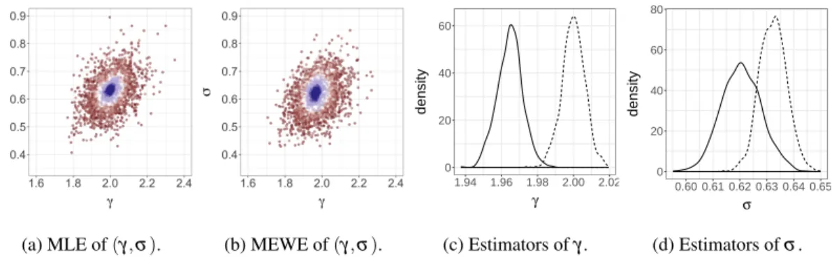
widely used in practice in the form of regression models. Figure4compares the sampling distributions of the maximum likelihood estimator and approximations of the MEWE of order 1, over M=1,000 experiments, for different values ofn. The MEWE converges at the same√nrate as the MLE, albeit to a distribution that is centered at a different location. Therefore, despite both estimation techniques leading to similar values forγandσ, the distributions of the estimators have very little overlap for large n, as observed in Figures4cand4d. For the MEWE, we have again usedm=104,k=20, and one iteration of MCEM.
In Figure5, we fix an observed data set of sizen=100, and computeM=500 instances of the approximate MEWE for 8 different values of k andm, ranging from 1 to 1,000 and 10 to 10,000 respectively. In Figure5a, we plot the estimators obtained for all the levels ofk, given 4 different values ofm. In Figure5b, we plot the estimators obtained for all the levels ofm, given 4 different values of k. The axis scales are different for each subplot. In both figures, black points correspond to the “true” MWE, calculated using a very large value ofm(m=108). For low values ofm, the estimators might be significantly different from the MWE, as can be seen from the lower-right sub-plots of Figure5b. When mincreases, the estimators converge to the MWE. Increasingkreduces variation in the estimator. The changes inkandmhad no significant impact on the number of evaluations of the objective required to locate the maximum using theoptimfunction inR(R Core Team,2015), which uses the Nelder–Mead simplex method (Nelder and Mead,1965).
We check the coverage of bootstrap confidence intervals calculated forθ?(itself calculated using n=m=108andk=1). As before, we use the percentile bootstrap (Efron and Tibshirani,1994) for
(a) MLE of(γ,σ). (b) MEWE of(γ,σ). 0 20 40 60 1.94 1.96 1.98 2.00 2.02 γ density (c) Estimators ofγ. 0 20 40 60 80 0.60 0.61 0.62 0.63 0.64 0.65 σ density (d) Estimators ofσ.
FIG. 4:Gamma data fitted with a Normal model, as described in Section4.3. Figures4aand4bshow the sampling distributions of the MLE and MEWE of order 1 respectively, asnranges from 50 to 104(colors from red to white
to blue). Figures4cand4dshow the marginal densities of the estimators ofγandσrespectively, forn=104; the MLEs are shown in dashed lines and the MEWE in full lines. For the MEWE, we have usedm=104,k=20 and
one iteration of MCEM.
data sets of sizen=1,000 and synthetic data sets of sizem=104, and calculate the MEWE withk=20.
We draw 400 data sets from the data-generating process, and 1,000 bootstrap data sets for each of these. The observed coverage rates of the resulting 0.95 confidence intervals were 0.960 and 0.953 forγ?and
σ?respectively. After a Bonferroni correction, the observed coverage rate of the confidence sets for
θ?= (γ?,σ?)was 0.955.
4.4 Cauchy data fitted with a Normal model
Let µ? be Cauchy with median zero and scale one, and consider the model M ={N (γ,σ2):γ∈
R,σ >0}. We explore the behavior of the MEWE of order 1, overM=1,000 repeated experiments.
Figure6shows its sampling distributions, fornranging from 50 to 104. The marginal distribution of the estimator ofγ concentrates around 0, the median ofµ?. The marginal distribution of the estimator ofσ also concentrates to a value close to 2.2. The concentration appears to occur at rate√n, as shown by the marginal densities of the rescaled estimators ofγandσin Figures6aand6b.
In this setting the maximum likelihood estimator would not converge asn→∞, as the maximum likelihood estimator forγ is the sample average, and the sample average of independent Cauchy vari-ables is also Cauchy, with the same location and scale. As an alternative, we consider an estimator defined by minimizing a sample based estimator of the Kullback-Leibler divergence betweenµθ and
µ?. For the KL approximation we use the functionKL.divergencein theFNNpackage (
Beygelz-imer et al.,2013), which approximates the KL divergence using`-nearest neighbor estimates described inBoltz et al.(2009) (and using the default parameter`=5). The resulting estimator is termed the minimum KL estimator (MKLE), and is a variation of the MDEs discussed byBasu et al.(2011). We compute it using the same approach as for the MEWE, usingk=20,m=104, and one iteration of MCEM. Forn=5,000 the distributions of MEWEs and MKLEs are plotted in Figures6cand6d. Both estimators appear to be robust in the sense that they converge to well-defined limits, unlike the MLE approach. The estimators ofγare concentrated around 0, but the estimators ofσare concentrated around
two different values: the MEWEs seem to concentrate around 2.15 and the MKLEs around 1.65. The marginal distributions of the MEWE appear to have slightly smaller variance than those of the MKLE.
(a) Approximate MEWE for increasingk (colors from red to white to blue askincreases), for dif-ferent values ofm.
(b) Approximate MEWE for increasingm(colors from red to white to blue asmincreases), for differ-ent values ofk.
FIG. 5: Gamma data withn=100, fitted with a Normal model, as described in Section4.3. MEWEs are obtained for different values ofm(from 10 to 10,000) andk(from 1 to 1,000), using one iteration of MCEM,M=500 times independently. The intersections of the black lines represent the location of the “exact” MWE computed with n=m=108.
0.00 0.05 0.10 0.15 −5 0 5 10 γ density
(a)√n-scaled estim. ofγ. 0.000 0.025 0.050 0.075 0.100 −10 0 10 20 σ density (b)√n-scaled estim. ofσ. 0 3 6 9 12 0.0 0.2 0.4 γ density (c) Estimators ofγ. 0 2 4 6 1.5 2.0 2.5 σ density (d) Estimators ofσ.
FIG. 6:Cauchy data fitted with a Normal model, as described in Section4.4. Marginals distributions of the MEWE ofγandσ, centered byθ?itself computed withn=m=108, and rescaled by√n, are shown in Figures6aand6b.
Figures6cand6dshow the distributions of the MEWE forn=5,000 (full lines), along with the distribution of an estimator obtained by minimizing an estimate of the Kullback–Leibler divergence (dashed lines).
Note that this example is not covered by the theoretical results of Section2since the Cauchy distribu-tion does not have a finite first moment. Robustness properties of general minimum distance estimators are discussed inParr and Schucany(1980), and of the MWE in location models inBassetti and Regazz-ini(2006). In the location-scale model considered here, if the approximation of the MEWE is computed withk=1 andm=`nfor some`>1, it can be written
argmin γ,σ n
∑
i=1 `∑
j=1 |y(i)−(σx(`(i−1)+j)+γ)|. (4.2)As such, the approximate MEWE can be seen as the coefficients in a median regression (Koenker and Hallock,2001) of a vector ˜Yon a vector ˜X, where ˜Y`(i−1)+1:`i=y(i)for eachi=1, . . . ,n, and ˜Xcontains the order statistics of anm-sample ofN (0,1)random variables. Quantile regression is often presented as a robust alternative to linear regression in the presence of outliers, and further connections might explain the observed robustness of the MEWE withp=1 in this example.
5. Discussion
The minimum Wasserstein (or Kantorovich) estimation approach (Bassetti et al.,2006) has received a renewed attention, due to recent advances in the field of computational optimal transport (Peyr´e and Cuturi,2018), along with various applications in machine learning. In the broad context of generative models, these estimators present various appeals compared to maximum likelihood estimators. For instance, in Sections 4.1and4.2, we have observed the satisfactory behavior of minimum expected Wasserstein estimators in models where the likelihood function is not analytically available. In Sections
4.3and4.4we have observed similarities and differences between MEWE and MLE in misspecified settings, illustrating some robustness properties of minimum Wasserstein estimation.
Minimum distance estimators were originally developed for obtaining almost surely convergent esti-mators (Wolfowitz,1957), and we have showed that both the MWE and MEWE have this strong consis-tency property under mild conditions. We have also proved that the MWE converges toθ?at the optimal √
The generalization of this result to multivariate data is left for future research. Interestingly, given the known convergence properties of the Wasserstein distance, it seems reasonable to conjecture that the rate of the MWE depends (negatively) on the dimension of the observation space rather than that of the parameter space. Other topics for future research include a more general derivation of the limiting distri-butions of the estimators, whose existence is needed to justify the asymptotic coverage of subsampling confidence intervals, as well as the development of a better understanding of their robustness properties.
Acknowledgements
The bootstrap experiments were in part performed on the Odyssey cluster supported by the FAS Division of Science, Research Computing Group at Harvard University. Pierre E. Jacob acknowledges support from the National Science Foundation through grant DMS-1712872.
References
Altschuler, J., Bach, F., Rudi, A., and Weed, J. (2018). Massively scalable Sinkhorn distances via the Nystr¨om method.arXiv preprint arXiv:1812.05189. 2,10
Altschuler, J., Weed, J., and Rigollet, P. (2017). Near-linear time approximation algorithms for optimal transport via sinkhorn iteration. InAdvances in Neural Information Processing Systems, pages 1964– 1974.10
Ambrosio, L., Gigli, N., and Savar´e, G. (2005). Gradient Flows in Metric Spaces and in the Space of Probability Measures. Birkh¨auser Verlag AG, Basel, second edition.5,9
Arjovsky, M., Chintala, S., and Bottou, L. (2017). Wasserstein generative adversarial networks. In Proceedings of the 34th International Conference on Machine Learning, volume 70, pages 214–223. PMLR. 2,4
Bassetti, F., Bodini, A., and Regazzini, E. (2006). On minimum Kantorovich distance estimators. Statis-tics & probability letters, 76(12):1298–1302. 1,4,5,17
Bassetti, F. and Regazzini, E. (2006). Asymptotic properties and robustness of minimum dissimilarity estimators of location-scale parameters. Theory of Probability and its Applications, 50(2):171–186.
2,4,6,17
Basu, A., Shioya, H., and Park, C. (2011).Statistical Inference: the Minimum Distance Approach. CRC Press. 2,3,15
Belili, N., Bensa¨ı, A., and Heinich, H. (1999). Estimation based on the Kantorovich functional and the L´evy distance. Comptes Rendus de l’Academie des Sciences Series I Mathematics, 5(328):423–426.
1
Benamou, J.-D., Carlier, G., Cuturi, M., Nenna, L., and Peyr´e, G. (2015). Iterative Bregman projec-tions for regularized transportation problems. SIAM Journal on Scientific Computing, 37(2):A1111– A1138. 2,10
Bernton, E., Jacob, P. E., Gerber, M., and Robert, C. P. (2019). Approximate Bayesian computation with the Wasserstein distance.To appear, Journal of the Royal Statistical Society: Series B.2,10,11
Bertsimas, D. and Tsitsiklis, J. N. (1997).Introduction to Linear Optimization. Athena Scientific. 9
Beygelzimer, A., Kakadet, S., Langford, J., Arya, S., Mount, D., and Li, S. (2013). FNN: fast nearest neighbor search algorithms and applications.R package version, 1.15
Bickel, P. J. and Sakov, A. (2008). On the choice of m in the m out of n bootstrap and confidence bounds for extrema.Statistica Sinica, pages 967–985.7
Boltz, S., Debreuve, E., and Barlaud, M. (2009). High-dimensional statistical measure for region-of-interest tracking. IEEE Transactions on Image Processing, 18(6):1266–1283.15
Bonneel, N., Rabin, J., Peyr´e, G., and Pfister, H. (2015). Sliced and radon Wasserstein barycenters of measures.Journal of Mathematical Imaging and Vision, 51(1):22–45. 10
Brown, L. D. and Purves, R. (1973). Measurable selections of extrema. Annals of Statistics, 1(5):902– 912.5
Burkard, R., Dell’Amico, M., and Martello, S. (2009).Assignment Problems. Society for Industrial and Applied Mathematics (SIAM).9
Chen, Y. and Li, W. (2018). Natural gradient in Wasserstein statistical manifold. arXiv preprint arXiv:1805.08380.11
Cheney, E. W. and Wulbert, D. E. (1969). The existence and unicity of best approximations. Mathemat-ica ScandinavMathemat-ica, 24:113–140.6
Cuturi, M. (2013). Sinkhorn distances: lightspeed computation of optimal transport. InAdvances in Neural Information Processing Systems (NIPS), pages 2292–2300.2,10
Dede, S. (2009). An empirical central limit theorem inl1for stationary sequences.Stochastic Processes and their Applications, 119:3494 – 3515. 6
del Barrio, E., Gin´e, E., and Matr´an, C. (1999). Central limit theorems for the Wasserstein distance between the empirical and the true distributions.Annals of Probability, pages 1009–1071. 6,7
del Barrio, E., Gin´e, E., Utzet, F., et al. (2005). Asymptotics forl2functionals of the empirical
quan-tile process, with applications to tests of fit based on weighted Wasserstein distances. Bernoulli, 11(1):131–189.6
del Barrio, E. and Loubes, J.-M. (2017). Central limit theorems for empirical transportation cost in general dimension.arXiv preprint arXiv:1705.01299.7,8
Devroye, L. (1985).Non-uniform random variate generation. Springer-Verlag, New York. 9
Efron, B. and Tibshirani, R. J. (1994).An Introduction to the Bootstrap. CRC press. 7,12,13,14
Fenton, L. (1960). The sum of log-Normal probability distributions in scatter transmission systems.IRE Transactions on Communications Systems, 8(1):57–67.13
Fournier, N. and Guillin, A. (2015). On the rate of convergence in Wasserstein distance of the empirical measure.Probability Theory and Related Fields, 162:707–738. 8
Genevay, A., Cuturi, M., Peyr´e, G., and Bach, F. (2016). Stochastic optimization for large-scale optimal transport. InAdvances in Neural Information Processing Systems (NIPS), pages 3432–3440. 2
Genevay, A., Peyr´e, G., and Cuturi, M. (2017). GAN and VAE from an optimal transport point of view. arXiv preprint arXiv:1706.01807. 2
Genevay, A., Peyre, G., and Cuturi, M. (2018). Learning generative models with Sinkhorn divergences. In Storkey, A. and Perez-Cruz, F., editors,Proceedings of the Twenty-First International Conference on Artificial Intelligence and Statistics, volume 84 ofProceedings of Machine Learning Research, pages 1608–1617.2,4,10
Gottschlich, C. and Schuhmacher, D. (2014). The shortlist method for fast computation of the earth mover’s distance and finding optimal solutions to transportation problems.PloS one, 9(10):e110214.
9
Gouri´eroux, C., Monfort, A., and Renault, E. (1993). Indirect inference. Journal of Applied Economet-rics, 8:85–118.2,3
Hansen, L. P. (1982). Large sample properties of generalized method of moments estimators. Econo-metrica: Journal of the Econometric Society, pages 1029–1054. 3
Jorge, M. and Boris, I. (1984). Some properties of the Tukey g and h family of distributions. Commu-nications in Statistics-Theory and Methods, 13(3):353–369.11
Koenker, R. and Hallock, K. F. (2001). Quantile regression. Journal of Economic Perspectives, 15(4):143–156.17
Le Cam, L. (1970). On the assumptions used to prove asymptotic normality of maximum likelihood estimators. Annals of Mathematical Statistics, 41:802–828.6
Li, W., Ryu, E. K., Osher, S., Yin, W., and Gangbo, W. (2018). A parallel method for Earth Movers distance.Journal of Scientific Computing, 75(1):182–197. 2,10
Marin, J.-M., Pudlo, P., Robert, C. P., and Ryder, R. J. (2012). Approximate Bayesian computational methods. Statistics and Computing, 22(6):1167–1180. 2
McFadden, D. (1989). A method of simulated moments for estimation of discrete response models without numerical integration. Econometrica, 57(5):995–1026.3
Neath, R. C. et al. (2013). On convergence properties of the Monte Carlo EM algorithm. InAdvances in Modern Statistical Theory and Applications: A Festschrift in Honor of Morris L. Eaton, pages 43–62. Institute of Mathematical Statistics.10
Nelder, J. A. and Mead, R. (1965). A simplex method for function minimization.The Computer Journal, 7(4):308–313. 14
Owen, A. B. (2001). Empirical likelihood. CRC press. 3
Parr, W. C. and Schucany, W. R. (1980). Minimum distance and robust estimation. Journal of the American Statistical Association, 75(371):616–624. 17
Peyr´e, G. and Cuturi, M. (2018). Computational Optimal Transport.arXiv preprint arXiv:1803.00567.
2,9,10,17
Politis, D. N., Romano, J. P., and Wolf, M. (1999).Subsampling. Springer-Verlag New York. 6
Pollard, D. (1980). The minimum distance method of testing.Metrika, 27:43–70.2,5,6
Puccetti, G. (2017). An algorithm to approximate the optimal expected inner product of two vectors with given marginals.Journal of Mathematical Analysis and Applications, 451(1):132–145.10
R Core Team (2015). R: A Language and Environment for Statistical Computing. R Foundation for Statistical Computing, Vienna, Austria.11,14
Rabin, J., Peyr´e, G., Delon, J., and Bernot, M. (2011). Wasserstein barycenter and its application to texture mixing. InInternational Conference on Scale Space and Variational Methods in Computer Vision, pages 435–446. Springer. 10
Ramdas, A., Trillos, N. G., and Cuturi, M. (2017). On Wasserstein two-sample testing and related families of nonparametric tests.Entropy, 19(2):47.10
Rayner, G. D. and MacGillivray, H. L. (2002). Numerical maximum likelihood estimation for the g-and-k and generalized g-and-h distributions.Statistics and Computing, 12(1):57–75. 11
Rockafellar, R. T. and Wets, R. J.-B. (2009). Variational Analysis, volume 317. Springer Science & Business Media.2
Rodrigues, G., Prangle, D., and Sisson, S. (2018). Recalibration: A post-processing method for approx-imate Bayesian computation.Computational Statistics & Data Analysis, 126:53–66.13
Rubio, F. J., Johansen, A. M., et al. (2013). A simple approach to maximum intractable likelihood estimation.Electronic Journal of Statistics, 7:1632–1654.11
Schuhmacher, D., Bhre, B., Gottschlich, C., and Heinemann, F. (2017). transport: Optimal Trans-port in Various Forms. R package version 0.8-2.9
Sisson, S. A., Fan, Y., and Beaumont, M. (2018). Handbook of Approximate Bayesian Computation. CRC Press.11
Tukey, J. W. (1977). Modern techniques in data analysis. InProceedings of the NSF-Sponsored Regional Research Conference, volume 7. Southern Massachusetts University.11
Van der Vaart, A. W. (2000).Asymptotic Statistics. Cambridge university press.5
Villani, C. (2008).Optimal Transport, Old and New. Springer-Verlag New York. 4
Weed, J. and Bach, F. (2019). Sharp asymptotic and finite-sample rates of convergence of empirical measures in Wasserstein distance.To appear, Bernoulli.7
Wei, G. C. and Tanner, M. A. (1990). A Monte Carlo implementation of the EM algorithm and the poor man’s data augmentation algorithms. Journal of the American Statistical Association, 85(411):699– 704.10
Wellner, J. A. and van der Vaart, A. W. (1996). Weak Convergence and Empirical Processes. Springer-Verlag New York. 6
Wolfowitz, J. (1957). The minimum distance method.The Annals of Mathematical Statistics, 28(1):75– 88.3,17
Wood, S. N. (2010). Statistical inference for noisy nonlinear ecological dynamic systems. Nature, 466(7310):1102–1104. 11
Ye, J., Wang, J. Z., and Li, J. (2017). A simulated annealing based inexact oracle for Wasserstein loss minimization. InProceedings of the 34th International Conference on Machine Learning, volume 70, pages 3940–3948. PMLR.2,10
List of Figures
1 Estimators in the well-specified g-and-κ model, as described in Section 4.1.1. Figures 1a and 1b show the MEWE’s bivariate marginal sampling distributions for(a,b)and(g,κ)respectively, asnranges from 50 to 104(colors from red to white to blue asnincreases). For eachn, we plotM=1,000 estimators based on independent data sets. Each estimator was computed with p=1,m=104,k=20, and one iteration of MCEM. Note that for small data sizes (n=50 and
n=100), the estimator occasionally appears to be on the boundary of the parameter space, which could mean that the optimization procedure failed to converge. The intersections of the black lines indicate data-generating parameters. Figure 1c shows the MEWE’s marginal distribution for
κ for the different levels ofn, centered and rescaled by√n, illustrating the rate of convergence
anticipated by Theorem 2.3. Figure 1d is a histogram of a data set generated withθ?= (3,1,2,0.5) andn=1,000. . . 12
2 Estimators in the g-and-κmodel with dependent data, as described in Section 4.1.2. Figures 2a
and 2b show the MEWE’s bivariate marginal sampling distributions for(a,b)and(g,κ)
respec-tively, asnranges from 500 to 105(colors from red to white to blue asnincreases). Note that the sample sizes here are 10 times larger than in the plots for the i.i.d. setting. For eachn, we plotM=1,000 estimators based on independent data sets. Each estimator was computed with p=1,m=104,k=20, and one iteration of MCEM. The intersections of the black lines indicate data-generating parameters. Figure 2c shows the MEWE’s marginal distribution forκfor the dif-ferent levels ofn, centered and rescaled by√n, illustrating the rate of convergence anticipated by Theorem 2.3, but that the asymptotic variance is larger than in the i.i.d. case. Figure 2d shows the autocorrelation function of a data set generated withθ?= (3,1,2,0.5),ρ=0.75, andn=1,000. 13
3 Estimators in the well-specified sum of log-Normals model, as described in Section 4.2. Figure 3a shows the sampling distributions of the MEWE, asnranges from 50 to 104(colors from red to white to blue asnincreases). For eachn, we plotM=1,000 estimators based on independent data sets. Each estimator was computed withp=1,m=104,k=20, and one iteration of MCEM. The intersections of the black lines indicate data-generating parameters. Figures 3b and 3c show the MEWE’s marginal distributions for the different levels ofn, centered and rescaled by√n, illustrating the rate of convergence anticipated by Theorem 2.3. Figure 3d is a histogram of a data set generated withθ?= (0,1)andn=1,000. . . 14
4 Gamma data fitted with a Normal model, as described in Section 4.3. Figures 4a and 4b show the sampling distributions of the MLE and MEWE of order 1 respectively, asnranges from 50 to 104 (colors from red to white to blue). Figures 4c and 4d show the marginal densities of the estimators ofγandσrespectively, forn=104; the MLEs are shown in dashed lines and the MEWE in full lines. For the MEWE, we have usedm=104,k=20 and one iteration of MCEM. . . 15
5 Gamma data withn=100, fitted with a Normal model, as described in Section 4.3. MEWEs are obtained for different values ofm(from 10 to 10,000) andk(from 1 to 1,000), using one iteration of MCEM,M=500 times independently. The intersections of the black lines represent the location of the “exact” MWE computed withn=m=108. . . 16
6 Cauchy data fitted with a Normal model, as described in Section 4.4. Marginals distributions of the MEWE ofγandσ, centered byθ?itself computed withn=m=108, and rescaled by√n, are
shown in Figures 6a and 6b. Figures 6c and 6d show the distributions of the MEWE forn=5,000 (full lines), along with the distribution of an estimator obtained by minimizing an estimate of the Kullback–Leibler divergence (dashed lines). . . 17