Evolutionary algorithms, simulated annealing and tabu search:
a comparative study
Habib Youssef*, Sadiq M. Sait, HakimAdiche
Department of Computer Engineering, KingFahd University of Petroleum and Minerals, KFUPM Box # 673, Dhahran-31261, Saudi Arabia
Received 1 July 1999; received in revised form1 June 2000; accepted 1 July 2000
Abstract
Evolutionary algorithms, simulated annealing (SA), and tabu search (TS) are general iterative algorithms for combinatorial optimization. The termevolutionary algorithmis used to refer to any probabilistic algorithmwhose design is inspired by evolutionary mechanisms found in biological species. Most widely known algorithms of this category are genetic algorithms (GA). GA, SA, and TS have been found to be very effective and robust in solving numerous problems from a wide range of application domains. Furthermore, they are even suitable for ill-posed problems where some of the parameters are not known before hand. These properties are lacking in all traditional optimization techniques. In this paper we perform a comparative study among GA, SA, and TS. These algorithms have many similarities, but they also possess distinctive features, mainly in their strategies for searching the solution state space. The three heuristics are applied on the same optimization problem and compared with respect to (1) quality of the best solution identified by each heuristic, (2) progress of the search frominitial solution(s) until stopping criteria are met, (3) the progress of the cost of the best solution as a function of time (iteration count), and (4) the number of solutions found at successive intervals of the cost function. The benchmark problem used is the floorplanning of very large scale integrated (VLSI) circuits. This is a hard multi-criteria optimization problem. Fuzzy logic is used to combine all objective criteria into a single fuzzy evaluation (cost) function, which is then used to rate competing solutions. # 2001 Elsevier Science Ltd. All rights reserved.
Keywords: Genetic algorithms; Simulated annealing; Tabu search; Fuzzy logic; Floorplanning; Combinatorial optimization; VLSI
1. Introduction
This paper is concerned with one class of combina-torial optimization algorithms: general iterative
al-gorithms, which constitute a class of approximation algorithms. The growing interest in this class of algorithms is attributed to their generality, ease of implementation, and mainly, their robustness in solving a wide variety of problems from a range of application domains. We shall limit ourselves to three popular iterative algorithms, (1) genetic algorithm, (2) simulated annealing, and, (3) tabu search. All three optimization heuristics have several similarities, namely (Sait and Youssef, 1999a):
1. They are approximation (heuristic) algorithms, i.e., they do not guarantee finding an optimal solution.
2. They are blind, in that they do not know when they reached an optimal solution. Therefore they must be told when to stop.
3. They have ‘‘hill climbing’’ property, i.e., they occasionally accept uphill (bad) moves.
4. They are general, i.e., they can easily be engineered to implement any combinatorial optimization problem; all that is required is to have a suitable solution representation, a cost function, and a mechanism to traverse the search space.
5. Under certain conditions, they asymptotically con-verge to an optimal solution.
The question of how to compare two constructive algorithms has long been settled. Two measures are typically used: (1) the time complexity of the algorithm, and, (2) the quality of solution, i.e., how far would the solution be fromoptimal in the worst or best case. In most cases, the time complexity of a constructive algorithmis usually easy to derive; however, determin-ing the quality of solution relative to the optimum is usually very difficult, and in some cases not possible.
*Corresponding author. Tel.: 4286; fax: +966-3-860-3059.
E-mail address:[email protected] (H. Youssef).
0952-1976/01/$ - see front matter # 2001 Elsevier Science Ltd. All rights reserved. PII: S 0 9 5 2 - 1 9 7 6 ( 0 0 ) 0 0 0 6 5 - 8
For iterative approximation algorithms, the time complexity is mostly a function of the number of iterations allowed for the algorithmas well as the complexity of the evaluation function. The various operators of the algorithmas well as the problemto be solved can also have determining effect on the time complexity of the algorithm. However, typically, all implementations of approximation iterative algorithms have polynomial time complexity. Thus the time complexity is not of concern when comparing heuristics in this category. Of major importance however is the quality of solution(s) found by a particular heuristic for the problemclass at hand. That is, if for example, a given iterative approximation algorithm A1 performs on average better than a second algorithmA2 over a number of problem instances, we then conclude that A1 implementation is better than that of A2. Another legitimate comparison would be with respect to the quality of the solution subspace examined by each algorithm. That is, if the number of solutions obtained with algorithmA1 with a cost lower than a particular value C is higher than that of algorithmA2, we then conclude that A1 exhibits superior performance than A2. Yet another comparison would be with respect to the progress of the best solution versus the number of iterations. In this paper we report a number of experiments performed to compare the performance of three well-known approximation iterative algorithms with respect to criteria such as those described above. The test problemused is floorplanning, a hard problem encountered during the physical design of VLSI circuits. It is encountered in several other areas of engineering as well. In VLSI design, a floorplanning tool helps decide several important questions such as dimensions, orien-tations and location of cells (or blocks), overall required area of the circuit, and speed performance requirements (Sait and Youssef, 1995).
The paper is organized as follows. Section 2 formulates floorplanning as a combinatorial optimiza-tion problem. In Secoptimiza-tion 3 we describe how a floor-planning solution is encoded and evaluated. The same solution encoding and evaluation function are used with all three approximation algorithms. Section 4 briefly discusses the main features and operators of each of GA, SA, and TS algorithms. In Section 5, experimental results are presented and the performance of the three heuristics are compared. We conclude in Section 6.
2. Floorplanning
A possible formulation of the floorplanning problem of VLSI circuits is as follows (Sait and Youssef, 1995):
Given:
1. A set of n rectangular blocks B¼ fb1;b2;. . .;
bi;. . .;bng; for eachbi2Bwe have
* wi;hi: width and height of bi, which are
constants for rigid blocks and variable for flexible blocks.
* r
i: desirable aspect ratio about each
variable-shape block where 1=ri4hi=wi4ri; ri¼1 if
blockiis rigid.
* ai: area ofbi (i.e.,ai¼wihi),ai is constant.
2. A set of nets N¼ fn1;n2;. . .;ni;. . .;nkg
describ-ing the connectivity information.
3. Desirable floorplan aspect ratio r such that 1=r4H=W4r; where H and W are the height and width of the floorplan, respectively.
4. Timing information.
Output: A legal floorplan is a floorplan satisfying the following constraints and objectives:
1. Each blockbi is assigned to a location (xi;yi);
2. no two blocks overlap;
3. for each flexible block bi; ai¼wihi;
4. meet aspect ratio constraints, for each flexible block bi and for the overall floorplan; and
5. minimize floorplan area, wire length and circuit delay.
Fig. 3(a) is a floorplan with 7 blocks.
3. Solution encoding and cost evaluation 3.1. Solution encoding
To have a simple and efficient encoding scheme the floorplanner constrains the structure to be slicing, but allows the circuit modules to have flexible shapes and free orientations. The layout is represented as a repetitive division into basic rectangles by horizontal and vertical cut-lines. Such a layout is called a slicing
structure. A slicing structure can be modeled by a binary tree with n leaves and n1 nodes, where each node represents a vertical cut-line or horizontal cut-line, and each leaf a basic rectangle. This binary tree is called
slicingtree, and the corresponding floorplan is aslicing
floorplan. Letters H and V refer to horizontal and vertical cut operators, respectively. A postorder traver-sal of a slicing tree produces a Polish expression with operators H and V, and with operands the basic rectangles 1;2;. . .;n(Wong and Liu, 1986). Fig. 3 gives a rectangular dissection, two possible slicing trees, and the corresponding Polish expressions. Since there is only one way of performing a postorder traversal of a binary tree, there is one-to-one correspondence between floor-plan trees and their corresponding Polish expressions. The operatorsH and V carry the following meanings:
ijH means rectangle j on-top-of rectangle i; ijV means rectangle i to-the-left-of rectangle j. In this work each solution is encoded as a Polish expression as in Wong and Liu (1986).
3.2. Cost evaluation
Unlike constructive algorithms for physical design, which produce a solution only at the end of the design process, iterative algorithms operate with design solu-tions defined at each iteration. An evaluation function is used to compare results of consecutive iterations and to select a solution based on the maximal (minimal) value of the objective function.
The cost function is a measure of how good is a particular floorplan. For floorplanning, three criteria are of prime importance: area, wire length, and timing. Area is estimated by the size of the smallest bounding rectangle of the floorplan. Wire length is set equal to the length of all the nets (or interconnects of the blocks) of the circuit. The length of an individual net or interconnect is estimated using the Steiner tree approx-imation of Youssef et al. (1995). The delay along the longest path of the circuit, taking into consideration the estimated interconnect length, is used as a measure of the timing performance of the floorplan (Youssef et al., 1995).
The cost function should reflect all objectives. Traditionally, multiple objectives have been combined into a scalar objective function, usually through a linear combination (weighted sum) of the multiple attributes, or by turning objectives into constraints. One way is to assign a constant weight to each of the multiple objective functions whose value will depend on the importance of that objective. Assuming that all objec-tives are to be maximized, the cost of a floorplan solutionxcan be expressed as follows:
costðxÞ ¼w1 f1ðxÞ þw2 f2ðxÞ þ þwn fnðxÞ; ð1Þ
wheren is the number of objective functions, and wi is
the weight of theith objectivefi. The problemwith this
weighted sumapproach is the difficulty in determining suitable weights. Adhoc methods are sometimes em-ployed.
Fuzzy logic. The logic used to infer a crisp outcome fromfuzzy input values is called fuzzy logic (Zadeh, 1965; Zimmermann, 1996; Kartalopoulos, 1996). Using fuzzy logic approach, optimization of a vector-valued function is replaced by the optimization of a scalar function, which is constructed fromthe levels of satisfaction of decision-makers by values of the compo-nents of a vector function. Below, we present a brief introduction to fuzzy logic, and then show how it can be applied in optimization problems with multiple objec-tives.
Fuzzy set theory: Unlike in ordinary set theory where an element is either in a set or not in a set, in fuzzy set theory, an element may partiallybelong to a set. Lotfi Zadeh defined a fuzzy set as a class of objects with a continuum of grades of membership. Formally, a fuzzy set Aof a universe of discourse X¼ fxg is defined as
A¼ fðx;mAðxÞÞjall x2Xg, where X is a space of points and mAðxÞ is a membership function of x2X
being an element of A. In general the membership functionmAð:Þis a mapping fromX to the interval [0,1]. IfmAðxÞ ¼1, or 0, for allx2X, the fuzzy setAbecomes an ordinary set (Zadeh, 1965).
Example. As an example, let h refer to height of an athlete, and ‘‘tall’’ considered as a particular value of the fuzzy variable ‘‘height’’. Then for each h in the range from0 to hmax, mtallðhÞ 2 ½0;1 indicates the extent to
which h is considered to be tall; mtallðhÞ is called the membership function.
Example. As another example, consider the possible heights of sportsmen in feet to be H ¼ f3:5;4:0;4:5;5:0;5:5;6:0;6:5g. Heights around 4.5 feet are considered short (S), around 5.5 feet are considered moderate (M), and heights around 6.0 feet are considered tall (T). Thus, short, moderate, and tall are
notcrisply defined. Fuzzy sets for short, moderate, and tall may be expressed as sets of ordered pairs
fðx;mAðxÞÞ jall x2Xg, where the first element of the
pair is the height and the second is its membership in that set. Fromour previous knowledge we can define the fuzzy setsS,M andT as follows:
S¼fð3:5;1:0Þ; ð4:0;1:0Þ; ð4:5;1:0Þ; ð5:0;0:3Þ; ð5:5;0:3Þ; ð6:0;0:0Þ; ð6:5;0:0Þg M¼fð3:5;0:0Þ; ð4:0;0:0Þ; ð4:5;0:1Þ; ð5:0;0:5Þ; ð5:5;1:0Þ; ð6:0;0:5Þ; ð6:5;0:1Þg T ¼fð3:5;0:0Þ; ð4:0;0:0Þ; ð4:5;0:0Þ; ð5:0;0:1Þ; ð5:5;0:4Þ; ð6:0;1:0Þ; ð6:5;1:0Þg
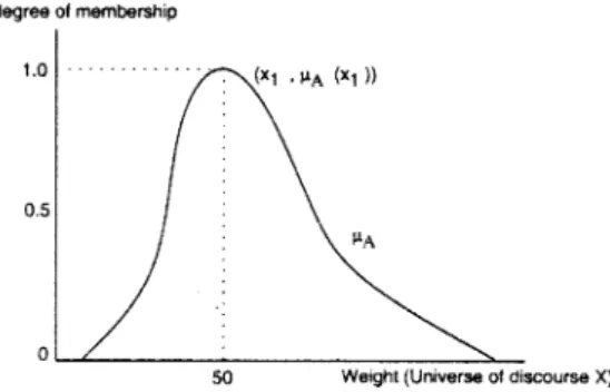
Fig. 1 illustrates the three membership functions. For simplicity we have used piecewise linear membership functions. Membership functions can also be continuous curves of many different shapes. For example, Fig. 2 illustrates a continuous membership function of a fuzzy set: An individual’s weight around 50 kg.
Fuzzy operators: As seen above, in fuzzy logic, the values are not crisp, and their fuzziness exhibits a distribution described by the membership function. In ordinary set theory, operations such as union ([), intersection (\), and complementation (:) are used. What is the result of these operations on fuzzy sets? This question has been addressed by various fuzzy logics. These are logics that have been defined for operations on fuzzy sets. One such logic defined by Zadeh is called themin–maxlogic (Zadeh, 1965). There are other fuzzy logics, one of which we used is discussed later. In
‘‘complementation’’ are defined as follows:
mA\BðxÞ ¼minðmAðxÞ; mBðxÞÞ; mA[BðxÞ ¼maxðmAðxÞ; mBðxÞÞ; m:AðxÞ ¼1:0 ðmAðxÞÞ:
Fuzzy rules: Approximate reasoning can be made based on linguistic variables and their values. Rules can be generated based on previous experience. Theserules
can then be expressed with If ... Then statements. Connectives such as AND and OR can be used in approximate reasoning to join two or more linguistic values.
As mentioned above, in min–max logic, the fuzzy
ANDis realized by the function min. If more than one rule is used to performdecision-making, each rule can be evaluated to generate a numerical value. Then, these numerical values from various evaluations of different rules can be combined to generate a crisp value on a higher level of hierarchy.
Fuzzification. In this work, we rely on the expressive power of fuzzy logic (Zadeh, 1965, 1975, 1973) to express the designer objectives in the formof fuzzy logic rules. The evaluation of a floorplanning solution consists of the evaluation of the fuzzy rules which return a value representing the degree of membership of that solution in the fuzzy subset of good floorplans. The fuzzy logic rules are expressed on linguistic variables of the problemdomain.
For floorplanning, the designer seeks to find floor-plans optimized with respect to the area occupied by the floorplan (area occupied by the cells and wires), wire length required to interconnet all the cells, and delay along the longest path of the corresponding circuit (delays due to the cells and wires). Therefore, the objective function is not a scalar, but a vector function
FðxÞ ¼ ðAreaðxÞ;LengthðxÞ;DelayðxÞÞ;
where x is a particular floorplan solution with area AreaðxÞ, wire length LengthðxÞ, and delay performance DelayðxÞ(Fig. 3).
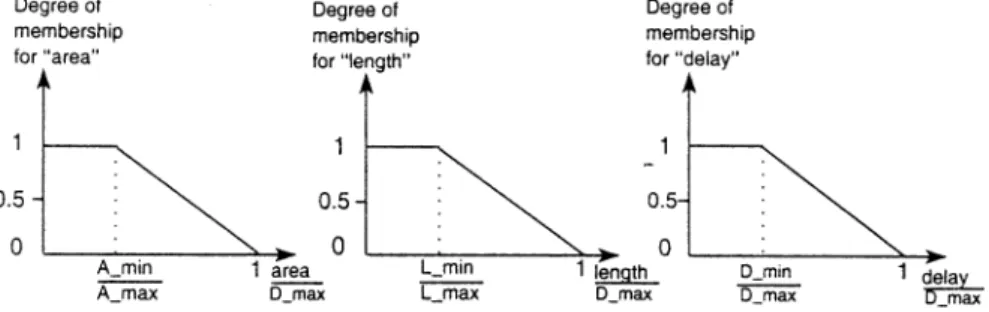
To obtain a fuzzy logic definition of the above multicriteria objective function, three linguistic variables area, length, and delay are defined Shragowitz et al., 1997). In this implementation, only one linguistic value is defined for each variable. That is, small area, short length, and low delay. These linguistic values character-ize the degree of satisfaction of the designer with the values of objectives Area, Length, and Delay of the floorplan. These degrees of satisfaction are described by membership functions mA; mL, andmD on fuzzy sets of linguistic values small area, short length, and low delay. Membership functions for small area, short length and low delay are easy to build. They are non-increasing functions, since the smaller the area, the length, and the delay, the higher is the degree of satisfactionmA,mL, and
mDof the expert and vice versa (see Fig. 4).
To make the membership functions applicable to different designs, the base variables floorplan area, length and delay are normalized to the interval [0,1] (see Fig. 4). The values Amin;Lmin, and Dmin are lower
bounds on the area, total length and clock period of the circuit. Amin is the sumof areas of all cells; Lmin is the
smallest possible length, computed assuming all con-nected cells are placed adjacent to each other;Dminis the
smallest possible delay of the circuit, which is the delay of the longest path due to cells and assuming minimum interconnect delay for the nets. The values of Amax,
Lmax, and Dmax are values corresponding to the initial
solution.
The most desirable floorplan is the one with the highest membership in the fuzzy subsets small area,
Fig. 1. Membership functions for short, moderate, and tall.
Fig. 2. Continuous membership function for the fuzzy set: individual’s weight around 50 Kg.
Fig. 3. (a) Slicing floorplan. (b) Slicing tree with Polish expression VH21HHV67V453. (c) Another possible slicing tree with Polish expression VH21HV67HV453.
short length and low delay. Such a solution most likely does not exist since some of the criteria conflict with each other. Therefore, one has to tradeoff these individual criteria against each other. This tradeoff is conveniently specified in linguistic terms in the form of one or several fuzzy logic rules.
As mentioned earlier, a fuzzy logic rule is anIf–Then
rule. TheIfpart (antecedent) is a fuzzy predicate defined in terms of linguistic values and fuzzy operators (AND
andOR). TheThenpart is called the consequent. In our case, the linguistic value used in the consequent part identifies the fuzzy subset of good solutions. Therefore, the result of evaluation of the antecedent part identifies the degree of membership in the fuzzy subset of good floorplan solutions according to the fuzzy rule in question (Shragowitz et al., 1997).
The fuzzy subset of good floorplan solutions is characterized by the following fuzzy rule:
R:0 Ifðsmall areaÞORðshort lengthÞORðlow delayÞ
Thengood solution:
According to the traditional min–max fuzzy logic, the above rule R.0 evaluates to the following:
mðSÞðxÞ ¼maxðmA;mL;mDÞ;
where mðSÞ is the membership function of the fuzzy subset of good solutions, and mA, mL, and mD are the membership functions in the fuzzy subsets of small-area solutions, short wire-length solutions, and small delay solutions, respectively. The min and max operators are non-compensatory, i.e., the weaker elements cannot compensate for the stronger element. Such property is undesirable in the case of multi-criteria optimiza-tion=decision problems. For this category of problems it is important to make use of all the information sources. In this case it is recommended to use a compensatory interpretation of the fuzzy OR operator, which allows all the criteria elements to influence the outcome of the operator. One such interpretation is the
orlike ordered weighted averaging (OWA) operator
suggested by Yager in Yager (1994); Yager and Filev (1994) in the context of the softening of the rule
aggregation technique. According to this orlike opera-tion, the fuzzy logic rule R.0 evaluates to the following:
mðSÞðxÞ ¼bmaxðm1;m2;m3Þ þ ð1bÞ 1 3 X3 i¼1 miðxÞ; ð2Þ
where mðSÞ is the membership function of the fuzzy
subset of good solutions, andbis a parameter between 0 and 1 indicating the degree of nearness of this orlike operator to the strict meaning of the logical OR operator. Whenb¼1, the orlike operator behaves like a regular max operator, and forb¼0 it behaves like a weighted averaging operator.
Individual objective criteria can be given relative ranking to reflect their importance. This can be achieved by assigning weights as exponents to individual mem-bership functions. When the memmem-bership function of a particular criterion is assigned a positive exponent less than 1, we say that the corresponding fuzzy subset is dilated. This corresponds to giving more empha-sis=importance to that criterion. Concentration corre-sponds to the case of assigning an exponent greater than 1 (Mendel, 1995). For example, in the case of floor-planning problem, Area is a more significant criterion, whereas Length and Delay are of equal but less importance. Such preferences can be conveniently expressed by using dilation and concentration operators. With these preferences, Eq. (2) becomes
mðSÞðxÞ ¼bmaxðm 1=2 A ;m2L;m2DÞ þ ð1bÞ 1 3ðm 1=2 A þm 2 Lþm2DÞ: ð3Þ
In the above equation, the fuzzy subset representing solutions with small area is dilated, whereas the fuzzy subset of solutions with short length and the fuzzy subset of solutions with small delay are concentrated.
4. GA, SA, AND TS algorithms
Any iterative approximation algorithm, be it GA, SA, or TS, requires decisions with respect to the following
elements:
* a solution encoding,
* a mechanism to generate initial solutions from where
the iterative search will proceed,
* an evaluation function to rate solutions encountered
during the search,
* perturbation operators to create new solutions froma
given current solution,
* assignment to the parameters of the algorithm, and * stopping criteria.
Below, we provide a brief description of each of GA, SA, and TS, and illustrate how each algorithmis adapted to the floorplanning problem.
4.1. Genetic algorithms
Genetic algorithms (GAs) are robust and effective optimization techniques inspired by the mechanism of evolution and natural genetics Goldberg, 1989; Holland, 1975. They are characterized by a parallel search of the state space as against a point-by-point search by the conventional optimization techniques. The parallel search is achieved by keeping a set of possible solutions to the optimization problem, called population. An individual in the population is a string of symbols and is an abstract representation of the solution. The symbols are called genes and each string of genes is termed achromosome. The individuals in the population are evaluated by some fitnessmeasure. The population of chromosomes evolves from generation to the next through the use of two types of genetic operators: (1) unary operators such as mutation and inversion which alter the genetic structure of a single chromosome, and (2) higher-order operator, referred to ascrossoverwhich consists of obtaining new individual by combining genetic material from two selected parent chromosomes. Then the new population is selected out of the indi-viduals of the current population and its offsprings. Based on the fitness value, two individuals (parents) are
selected at a time from the population. The genetic operators (crossover and mutation) are applied on the selected parents to generate new possible solutions called
offsprings. The structure of basic GA is given in Fig. 5. The application of genetic algorithmfor any problem requires a representation of the solution to the problem as a string of symbols, a choice of genetic operators, an evaluation function, a selection mechanism, and deter-mination of genetic parameters (population size and probabilities of crossover, mutation, and inversion). Each of these greatly influences the performance of the genetic algorithm.
In this work, a chromosome in the population (solution) is a Polish expression representing a particular slicing floorplan (see Section 3.1, Fig. 3). The initial population consists of randomly generated Polish
expressions with n operands and n1 operators. The fitness function is a measure of how good each individual of current generation is with respect to the desired features. For each chromosome x; fitness
ðxÞ ¼mðSÞðxÞ, where mðSÞ is as defined in Eq. (3). The
choice of parents fromthe set of individuals that comprise the population (also known as the mating pool) is probabilistic. In keeping with the ideas of natural selection, we assume that stronger individuals, that is, those with higher fitness values, are more likely to mate than the weaker ones. One way to simulate this is to select parents with a probability that is directly proportional to their fitness values. This method is called theroulette-wheel method(Goldberg, 1989).
Crossover. Crossover is a mechanism for probabilistic inheritance of useful information from two fit indi-viduals to offsprings. The main idea is that the genetic information of a good solution is spread over the entire population. Thus, the best solution can be obtained by thoroughly combining the chromosomes in the popula-tion. Crossover operation achieves recombination of the genetic material. The recombination process includes domain specific knowledge to enforce the inheritance of desirable features fromindividuals of current popula-tion. The following three crossover operators have been used in this work (Cohoon et al., 1991).
In the first crossover scheme, the operands from parent P1 are copied into the offspring O. Then, the
operators fromparentP2are copied by making a
left-to-right scan to complete the chromosome. Hence, each offspring inherits the block structure of one of the parents. For example, if P1¼VH21HHV67V453 and
P2¼VH12HV47HV653, then, according to this
cross-over, the offspring would beVH21HVH67V453. The second crossover operates by copying the operators fromparent P1 into the corresponding
positions in offspring O. Then, it completes the construction ofOby copying the operands fromparent
P2 by making a left-to-right scan. By propagating
the groups of operators from P1 to O, this
cros-sover produces an offspring having the same overall slicing structure as that of P1. We call this crossover
‘‘slicing inheritance crossover’’. For example, if
P1¼VH21HHV67V453 and P2¼VH12HV47HV653,
then, according to this crossover, the offspring would be
VH12HHV47V653. Both the above crossovers produce valid Polish expressions.
The third crossover employed in this work is the PMX crossover (partially mapped crossover) which has been widely used in other genetic implementations for combinatorial optimization problems (Shahookar and Mazumder, 1991). PMX is applied only on the modules (operands), the operators and the positions fromone of the parents are used in the offspring (see Figs. 6 and 7).
Mutation. Mutation is a means of introducing new information into the population. Three simple mutation
operators are used in this work (Wong and Liu, 1986): (1) inversion of a randomly selected chain of operators, (2) swapping of two randomly selected operands, and (3) swapping an operand with an adjacent operator (provided it results in a valid Polish expression).
Inversion. This operator consists of randomly select-ing two positions within the strselect-ing (a chromosome) and then laterally inverting the string between them. In this work, it is implemented so as to make a full right-to-left or left-to-right lateral inversion on the entire string of
operands (only). For example, if the chromosome before inversion is 268HH7H5V4H13VV, then after inversion the new solution generated will be: 314HH5H7V8H62VV. A number of methods have been proposed to select individuals that can survive and be used in the next generation (Goldberg, 1989). In this work, among the parents and their offsprings, the chromosomes for the next generation are chosen based on their fitness values
(higher fitness translates to higher survival). The probability of mutation is set to 5%, and the prob-ability of crossover to 80%. Inversion is applied with a probability of 30%. Population size chosen is 10, and in each generation the number of offsprings produced is the same as the number of parents. Stopping criterion in this case was set to a fixed number of generations.
Fig. 6. Crossover that propagates slicing structure to the offspring.
4.2. Simulated annealing
Simulated annealing (SA) is an iterative search method inspired by the annealing of metals (Kirkpatrick et al., 1983; Cerny, 1985). Starting with an initial solution and armed with adequate perturbation and evaluation functions, the algorithmperforms a stochas-tic partial search of the state space. Uphill moves are occasionally accepted with a probability controlled by a parameter called temperature ðTÞ. The probability of acceptance of uphill moves decreases asT decreases. At high temperature, the search is almost random, while at low temperature the search becomes almost greedy. At zero temperature, the search becomes totally greedy, i.e., only good moves are accepted (Kirkpatrick et al., 1983; Cerny, 1985).
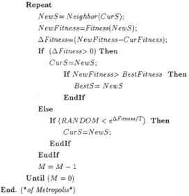
The basic SA algorithmis shown in Fig. 8. The core of the algorithmis the Metropolis procedure, which simulates the annealing process at a given temperature
T (Fig. 9) Metropolis et al., 1953. This procedure is named after the scientist who devised a similar scheme to simulate a collection of atoms in equilibrium at a given temperature. TheMetropolisprocedure receives as input the current temperature T, and the current solution CurS which it improves through local search.
Metropolis must also be provided with the value M, which is the amount of time for which annealing must be applied at temperatureT. The procedure Simulated_an-nealing simply invokes Metropolis at decreasing
tem-peratures. Temperature is initialized to a valueT0at the
beginning of the procedure (explained below), and is slowly reduced (in a geometric progression); the par-ameterais used to achieve this cooling. The amount of time spent in annealing at a temperature is gradually
increasedas temperature is lowered. This is done using the parameter b>1. The variable Time keeps track of the time being expended in each call to theMetropolis. The annealing procedure halts when Time exceeds the allowed time.
TheMetropolis procedure is shown in Fig. 9. It uses the procedure Neighbor to generate a local neighbor NewS of any given solution S. The function Fitness returns the fitness of a given solutionS. If the fitness of the new solution NewS is better than the fitness of the current solution Sc, then the new solution is accepted,
and we do so by setting CurS¼NewS. If the fitness of the new solution is better than the best solution (BestS) seen thus far, then we also replace BestS by NewsS. If the new solution has a lower fitness in comparison to the original solution CurS, Metropoliswill accept the new solution on a probabilistic basis. A randomnumber is generated in the range 0 to 1. If this randomnumber is smaller than eDfitness=T, where Dfitness¼fitness
ðNewSÞ FitnessðcurSÞ, andT is the current tempera-ture, the inferior solution is accepted. This criterion for accepting the new solution is known as the Metropolis criterion. The Metropolis procedure generates and examinesM solutions.
Initial temperature. The SA algorithmneeds to start froma high temperature ðTÞ. However, if this initial value of T is too high, it causes a waste of processing time. The initial temperature value should be such that it allows virtually all proposed uphill or down hill moves to be accepted. The temperature parameter is initialized using the procedure described in Wong and Liu (1986). The idea is basically to use the Metropolis function
(eDFitness=T) to determine the initial value of the
temperature parameter. Before the start of actual SA procedure, a constant number of moves, sayM, in the neighborhood of the current solution are made, and the respective fitness values of these moves are determined. The fitness difference for each movei; DFitnessiis given
byDFitnessi¼FitnessiFitnessi1. LetMuandMdbe
the number of uphill and downhill moves, respectively (downhill refers to inferior moves) (M¼MuþMd).
The average DFitnessd is then given by
DFitnessd¼ 1 Md XMd i¼1 DFitnessi:
Since we wish to keep the probability, say P0, of
accepting uphill moves high in the initial stage of SA, we estimate the value of the temperature parameter by substituting the value ofP0 in the following expression
derived fromthe Metropolis function:
T0¼
DFitnessd
lnðP0Þ ;
whereP01ðP0¼0:999Þ.
Parameters, stopping criterion. The parameter a for updating the temperature is user specified. In our implementation a takes on the value of 0.85, and b is set equal to 1. At each updated value of the temperature,
a number of state transitions are made so as to reach the probabilistic steady state.
The perturb mechanisms employed are similar to the mutation operators in GA. The stopping criterion is when the finalT50:001 orAt=Mt50:05, whereAtis the
total number of all accepted moves (both good and bad) and Mt is the number of all moves made at a given
temperature.
4.3. Tabu search
Tabu search is a higher-level method or meta strat-egy for solving combinatorial optimization problems (Glover, 1989, 1990). It is an iterative procedure that starts from some initial feasible solution and attempts to determine a better solution. TS makes several neighbor-hood moves and selects the move producing the best solution among all candidate moves for current itera-tion. This best candidate solution may not improve the current solution.
Selecting the best move (which may or may not improve the current solution) is based on the suppo-sition that good moves are more likely to reach the optimal or near-optimal solutions. The set of admissible solutions attempted at a particular iteration forms a
candidate list. TS selects the best solution fromthe
candidate list.Candidate list size is a trade-off between quality and performance.
To avoid move reversals, a device called tabu restriction is used that makes selected attributes of these moves tabu (forbidden). Tabu restrictions allow the search to go beyond the points of local optimality while still making the best possible move in each iteration. Tabu restrictions are enforced by atabu listwhich stores the move attributes to avoid move reversals. Tabu list has an associated size and can be visualized as a window on accepted moves. The moves which tend to undo moves within this window are forbidden.
Aspiration level component is used to temporarily override the tabu status if the move is sufficiently good. If a move is made tabu in iteration i and its reversal comes in iterationj, wherej5iþc, (wherecis the size of the tabu list), then it is possible that the reverse move may take the search into a new region because of the effects ofcintermediate moves. The simplest aspiration criterion, also known as the ‘‘best cost aspiration criterion’’, consists of overriding the tabu status if the reversal produces a solution better than the best obtained thus far. Another approach is to use the same attribute of the move which is used to identify the tabu status and associate an aspiration level value with it. The reversal has to do better than this historical aspiration level. Fig. 10 illustrates the flow of the short-termtabu search algorithm.
Only short-term tabu search was implemented in this work. The programis executed for 250 iterations. The
size of the candidate list was 20. Three perturbation schemes similar to the mutation scheme of GA (and also used in our implementation of SA) were used to generate neighborhood solutions. The size of the tabu list was set toN=4, whereNis the number of blocks in the floorplan. For each of the perturbation schemes a separate tabu list is used. The attributes stored in the tabu lists are related to the perturbation scheme. In the case where perturbation consists of inverting a chain of operators, the attribute stored is the position of the first operator of the chain. For the case of swapping two randomly selected operands, the attribute consists of one of the operands (the left operand) involved in the swap. The attribute related to the case of swapping an operand with an operator, is the operand. For all test
cases, the three tabu lists have the same size, and best cost aspiration criterion was used.
5. Experiments and results
The algorithms described in this paper were im-plemented and tested on five different VLSI circuits. The circuits range in sizes between 15 and 141 blocks. The characteristics of these circuits are summarized in Table 1. All three approximation algorithms GA, SA, and TS, make use of quite a bit of heuristic knowledge about the problemdomain. The existence of several alternative decisions with respect to each aspect of a particular algorithm(e.g., initial solution, operators, evaluation functions, etc.) strongly suggests that some implementa-tion of the same algorithm may perform better than other implementations. In this work, we compare the performance of the three algorithms with respect to the following aspects:
1. quality of the best solution identified by each heuristic,
2. progress of the search frominitial solution ðsÞ until stopping criteria are met,
3. the progress of the cost of the best solution as a function of time (iteration count), and
4. the number of solutions found at successive intervals of the cost function.
Fig. 11 is a plot of the fuzzy cost function (membership in the fuzzy subset of good floorplans) of the best floorplan versus the number of calls to the evaluation functions (number of solutions searched). With respect to this measure, tabu search ranked first, genetic algorithmsecond, and simulated annealing third. The same ranking was obtained with all five circuits. Fig. 11 shows results for two of the circuits, Ckt-3 (39 blocks) and Ckt-4 (45 blocks). Recall that the GA, SA, and TS floorplanners are seeking floorplan solutions with the largest membership function in the fuzzy subset of good floorplans.
The experimental results reported in this section are based on a GA implementation identical to that reported in Shragowitz et al. (1997). The SA implemen-tation is based on the work reported in Wong and Liu
Fig. 10. Flowchart of the short-termTabu search algorithm.
Table 1
Characteristics of circuits used
Ckt name No. of cells Amin Lmin Tmin
Ckt-1 15 34 800 960.16 34.04
Ckt-2 30 40 832 2325.76 28.95
Ckt-3 39 90 480 4283.86 11.60
Ckt-4 45 88 160 4430.31 16.57
(1986). For all experiments, the algorithm was forced to stop after 5000 evaluations.
Fig. 12 illustrates another performance aspect of the three heuristics. For GA algorithm, Fig. 12(a) and (d) show the variation of the population fitness versus the number of generations. For the SA algorithms, Fig. 12(b) and (e) show the cost of the current floorplan solution after every twenty iterations. For the TS heuristic, Fig. 12(c) and (f) show the cost of the solution selected at each iteration (the best floorplan in a
neighborhood of 20 floorplans). The reader should observe that TS quickly finds a good floorplan with a high membership value in the fuzzy subset of good solutions, and once there, the magnitude of uphill moves is always very small. In contrast, SA exhibits the most probabilistic behavior since relatively large uphill moves continue to be accepted even at relatively low tempera-tures. This undesirable behavior is partly due to the fact that the cost function is normalized to the range (0,1). Hence, though a decrease in the membership function
Fig. 11. Value of the membership functionmðSÞof the best solution as a function of the number of solutions examined. (a) Results for Ckt-3 with 39
blocks; (b) results for Ckt-4 with 45 blocks.
Fig. 12. Comparison of search paths of GA, SA, and TS. (a) and (d): GA average population cost versus number of generations for Ckt-3 and Ckt-4; (b) and (e): SA solution cost for every 20 iterations for Ckt-3 and Ckt-4; (c) and (f): cost of TS solutions at each iteration, where each iteration selects the best in a neighborhood of 20 solutions, for Ckt-3 and Ckt-4.
mðSÞ say from0.6 to 0.4 is considered large in the fuzzy
domain, may still produce a large acceptance probability according to the Metropolis function. For example, at
T ¼0:1; e0:2=0:1¼0:14. This suggests that the fuzzy
cost difference in the exponent of the Metropolis function be multiplied by an inflation factor. The inflation factor should be such that, in the cold regime, the probability of accepting large and even medium uphill moves be very near zero. We have conducted such experiment and used an inflation factor of 100. Hence, floorplan cost will no longer be in the range of (0,1) but in the range of (0,100). Fig. 13 illustrates the effect of using such an inflation factor on the performance of SA
algorithms. Fig. 13(a) compares the cost of the best floorplan as a function of the number of iterations, with and without the use of inflation factor in the Metropolis function. As the reader can see, results have significantly improved. Figs. 13(c) and 14(b) show that the quality of the searched subspace has also improved. Furthermore, a decrease in the magnitude of the accepted bad moves has also been observed; the reader is referred to the plots of Figs. 12(b) and 13(b).
For GA, the population fitness improves quickly in the first 200 iterations and then it hits a plateau. Further, in the first 50 generations the population fitness is steadily increasing; in the following generations the
Fig. 13. Results illustrating the effect of inflating the fuzzy cost on performance of SA algorithm. (a) Comparison of the fuzzy cost of the best floorplan with and without the use of inflation factor. (b) SA solution cost for every 20 iterations when the fuzzy cost is inflated. (c) Bar chart of SA with inflated fuzzy cost.
Fig. 14. Bar charts for GA, SA and TS depicting the sub-space searched by each heuristic. Thex-axis ismðSÞand they-axis indicates the number of solutions at a particular range ofmðSÞ. Recall that the higher the value ofmðSÞthe better is the corresponding floorplan solution. (a)–(c) are charts of test circuit Ckt-3 and (d)-(f) are charts of circuit Ckt-4.
population fitness occasionally decreases, however the magnitude of the decrease is relatively small (40:05). Similar plots were obtained for all circuits. These experiments confirm the fact that, although all three heuristics have hill climbing property, TS is the most greedy and SA is the least greedy.
A final series of experiments consists of comparing the three heuristics with respect to the searched solution subspaces. The results are summarized in Fig. 14 in the formof bar charts. Here again, TS exhibited the best performance and SA the worst. These bar charts are very informative as to where each algorithm spent its time. Both GA and TS concentrated their search efforts in good subspaces, that is, evaluating solutions with high membership in the fuzzy subset of good solutions. In contrast, SA spent most of its time evaluating poor quality solutions. This behavior was observed with all test cases.
6. Discussion & conclusion
In this paper, an experimental comparative study of three popular approximation algorithms is presented, viz., GA, SA, and TS for the floorplanning problem. All three heuristics assume and exploit regularities present within the search space, i.e., search spaces where good solutions have higher probabilities of leading to better solutions. All three have been found to be effective and robust on problems where some measure of progress can be shown. All or nothing types of search spaces where one either has a perfect solution or no solution are better attacked by exhaustive search or even by randomwalk. The three algorithms discussed incorporate domain specific knowledge to dictate the search strategy. They also tolerate some element of non-determinism that helps the search escape out of local minima. They rely on the use of a suitable cost function which provides feedback to the algorithmas the search progresses. The principle difference among them is how and where domain-specific knowledge is used. For example, in simulated annealing such knowledge is mainly included in the cost function. Elements involved in a perturbation are selected randomly, and perturbations are accepted or rejected according to the Metropolis criterion which is a function of the cost. The cooling schedule has also a major impact on the algorithm performance and must be carefully crafted to the problemdomain as well as the particular probleminstance.
In the case of genetic algorithms, domain specific knowledge is exploited in all phases. The fitness of individual solutions incorporates domain-specific knowledge. Selection for reproduction, the genetic operations, as well as generation of the new population also incorporate a great deal of heuristic knowledge about the problemdomain.
Tabu search is different fromthe above heuristics in that it has an explicit memory component. At each iteration the neighborhood of the current solution is partially explored, and a move is made to the best non-tabu solution in that neighborhood. The neighborhood function as well as tabu list size and content are problem specific. The direction of the search is also influenced by the memory structures.
In this work our intention has been to study the behavior of the three heuristics in solving a hard engineering problem, and not to demonstrate the superiority of one algorithmover the other over all problemdomains. Each one of themhas its merits. Actually it would be unwise to generalize the results reported here over all classes of problems. We believe that some heuristics are easier to engineer to solve a particular problemthan others. For the benchmark problemused in this work tabu search exhibited better overall behavior than GA and SA.
Recently, an interesting theoretical study has been reported by Wolpert and Macready in which they proved a number of theorems stating that the average performance of any pair of iterative (deterministic or non-deterministic) algorithms across all problems is identical. That is, if an algorithmperforms well on a certain class of problems then it necessarily pays for that with degraded performance on the remaining set of problems (Wolpert and Macready, 1997). However, it should be noted that the reported theorems assume that the algorithms do not include domain-specific knowl-edge of the problems being solved. Obviously, it would be expected that a well-engineered algorithmwould exhibit superior performance to that of a poorly engineered one. Further, they do not assume any knowledge about the problems themselves. However the problemmaybe trivially stated that any algorithm would be able to find a solution to the problem.
Of the three heuristics experimented with in this work, TS exhibited the best performance with respect to solution quality as well as the quality of the solution subspace searched. Furthermore, with respect to the complexity of implementation and tuning of the algorithms parameters, GA required the most effort. SA and TS required similar and lesser efforts than GA. On the basis of experiments performed, and for the target problemcategory (floorplanning), TS is the better of the three heuristics, with GA a close second, and SA a distant third. Would the same verdict hold over other problemcategories? To answer such question would require at least that similar experiments on other category of problems be performed. Such experiments are the subject of future work. Also, similar study of other iterative approximation algorithms such as simu-lated evolution and stochastic evolution are being conducted (Sait and Youssef, 1999b; Kling and Ban-erjee, 1989; Saab and Rao, 1991).
Acknowledgements
The authors acknowledge King Fahd University of Petroleumand Minerals, Dhahran, Saudi Arabia, for support.
References
Cerny, V., 1985. Thermodynamical approach to the traveling salesman problem: an efficient simulation algorithm. Journal of Optimization Theory and Application 45 (1), 41–51.
Cohoon, J.P., Hedge, S.U., Martin, W.N., Richards, D., 1991. Distributed genetic algorithms for the floorplan design problem. IEEE Transactions on Computer-Aided Design 10 (4), 483–492.
Glover, F., 1989. Tabu search}Part I. ORSA Journal on Computing 1 (3), 190–206.
Glover, F., 1990. Tabu search}Part II. ORSA Journal on Computing 2 (1), 4–32.
Goldberg, D.E., 1989. Genetic Algorithms in Search, Optimization and Machine Learning. Addison-Wesley Publishing Company, Inc., Reading, MA.
Holland, J.H., 1975. Adaptation in Natural and Artificial Systems. University of Michigan Press, Ann Arbor, MI.
Kartalopoulos, S.V., 1996. Understanding Neural Networks and Fuzzy Logic}Basic Concepts and Applications. IEEE Press, New York.
Kirkpatrick Jr., S., Gelatt, C., Vecchi, M., 1983. Optimization by simulated annealing. Science 220 (4598), 498–516.
Kling, R.M., Banerjee, P., 1989. ESP: Placement by Simulated Evolution. IEEE Transactions on Computer-Aided Design 8 (3), 245–255.
Mendel, J., 1995. Fuzzy logic systems for engineering: a tutorial. Proceedings of the IEEE 83 (3), 345–377.
Metropolis, N., Rosenbluth, A., Rosenbluth, M., Teller, A., Teller, E., 1953. Equation of state calculations by fast computing machines. Journal of Chemical Physics 21, 1087–1092.
Saab, Y.G., Rao, V.B., 1991. Combinatorial Optimization by Stochastic Evolution. IEEE Transactions on Computer-Aided Design 10 (4), 525–535.
Sait, S.M., Youssef, H., 1999a. VLSI Physical Design Automation: Theory and Practice. McGraw-Hill Book Co., Europe (also co-published by IEEE Press, New York) 1995 (reprinted with corrections by World Scientific 1999).
Sait, S.M., Youssef, H., 1999b. Iterative Computer Algorithms for Optimization Problems. IEEE Computer Society Press, Silver Spring, MD.
Shahookar, K., Mazumder, P., 1991. VLSI cell placement. ACM Computing Surveys 23 (2), 143–220.
Shragowitz, E., Youssef, H., Sait, S.M., Adiche, H. 1997. Fuzzy genetic algorithmfor floorplan design. Proceedings of the 1997 SPIE International Symposium, Applications of Soft Computing and Fuzzy Logic Technology. San Diego, CA, Vol 3165, 27 July–1 August, pp. 36–46.
Wolpert, D.H., Macready, W.G., 1997. No free lunch theorems for optimization. IEEE Transactions on Evolutionary Computation 1 (1), 67–82.
Wong, D.F., Liu, C.L., 1986. A new algorithmfor floorplan design. Proceedings of the 23rd DAC. pp. 101–107.
Yager, R.R., 1994. On ordered weighted averaging aggregation operators in multicriteria decision making. IEEE Transactions on Systems, Man, and Cybernetics. SMC-18, pp. 183–190.
Yager, R.R., Filev, D.P., 1994. Parameterized andlike and orlike OWA operators. International Journal of General Systems 22, 297–316.
Youssef, H., Sait, S.M., Al-Farra, K., 1995. Timing Influenced force directed floorplanning. European Design Automation Conference with Euro-VHDL, Euro-DAC’95, Brighton, September, pp. 156– 161.
Zadeh, L.A., 1965. Fuzzy sets. Information and Control 8, 338–353. Zadeh, L.A., 1973. Outline of a new approach to the analysis of
complex systems and decisions processes. IEEE Transactions on Systems, Man, and Cybernetics SMC-3 (1), 28–44.
Zadeh, L.A., 1975. The concept of a linguistic variable and its application to approximate reasoning}I. Information Sciences 8, 199–249.
Zimmermann, H.J., 1996. Fuzzy Set Theory and its Applications, 2nd Edition. Kluwer Academic Publishers, Dordrecht.