Structure learning of graphs for count data

(1)

Sede Amministrativa: Universit`a degli Studi di Padova

Dipartimento di Scienze Statistiche

Corso di Dottorato di Ricerca in Scienze Statistiche Ciclo XXX

Structure Learning of Graphs for Count

Data

Coordinatore del Corso: Prof. Nicola Sartori Supervisore: Prof. Monica Chiogna

Dottoranda: NGUYEN Thi Kim Hue

(2)

(3)

Abstract

Biological processes underlying the basic functions of a cell involve complex interactions between genes. From a technical point of view, these interactions can be represented through a graph where genes and their connections are, respectively, nodes and edges.

The main research objective of this thesis is to develop a statistical framework for modelling the interactions between genes when the activity of genes is measured on a discrete scale. We propose several algorithms. First, we define an algorithm for learning the structure of a undirected graph, proving its theoretical consistence in the limit of infinite observations. Next, we tackle structure learning of directed acyclic graphs (DAGs), adopting a model specification proved to guarantee identifiability of the models. Then, we develop new algorithms for both guided and unguided structure learning of DAGs. All proposed algorithms show promising results when applied to simulated data as well as to real data.

(4)

(5)

Sommario

I processi biologici che regolano le funzioni di base di una cellula sono caratterizzati da numerose interazioni tra geni. Da un punto di vista matematico, `e possibile rap-presentare queste interazioni attraverso grafi in cui i nodi e gli archi rappresentano, rispettivamente, i geni coinvolti e le loro interazioni.

L’obiettivo principale di questa tesi è quello di sviluppare un approccio statistico alla modellazione delle interazioni tra geni quando questi sono misurati su scala discreta. Vengono a tal fine proposti vari algoritmi. La prima proposta è relativa ad un algoritmo disegnato per stimare la struttura di un grafo non orientato, per il quale si fornisce la dimostrazione di convergenza al crescere delle osservazioni. Altre tre proposte coin-volgono la definizione di algoritmi supervisionati per la stima della struttura di grafi direzionali aciclici, basati su una specificazione del modello statistico che ne garantisce l’identificabilità. Sempre con riferimento ai grafi direzionali aciclici, infine, si propone un algoritmo non supervisionato. Tutti gli algoritmi proposti mostrano risultati pro-mettenti in termini di ricostruzione delle vere strutture quando applicati a dati simulati e dati reali.

(6)

(7)

(8)

(9)

Acknowledgements

I would like to thank my supervisor, Professor Monica Chiogna, for her patience, en-couragement and advice in the past three years. She provided endless support, skilful guidance, and research freedom to me. Her extensive knowledge, enthusiasm have in-spired me throughout this PhD project.

I thank my colleagues from Department of Statistical Sciences, University of Padova. I feel incredibly lucky to have shared these three years of ups and downs with such an amazing group of people. I thank Vera for her help and encouragement at various times. I thank Elisa for her help on the analysis of gene sequencing data. I thank my Vietnamese friends for having funny and crazy activities together.

(10)

(11)

List of Figures

1.1 An example of a conditional independence displayed graphically . . . 6 3.1 The graph structures for p= 10 employed in the simulation studies: (a)

scale-free; (b) hub; (c) random graph. . . 44 3.2 The graph structures for p= 100 employed in the simulation studies: (a)

scale-free; (b) hub; (c) random graph. . . 44 3.3 Number of TP edges recovered by PC-LPGM; LPGM; PDN; VSL; GLASSO;

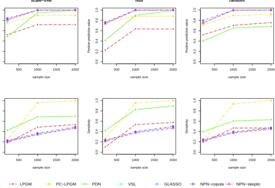
NPN-Copula; NPN-Skeptic for networks in Figure 3.1 (p = 10) and sample sizes n = 200,1000,2000. First panel row corresponds to high SNR level (λnoise = 0.5); second panel row corresponds to low SNR level

(λnoise = 5). . . 46

3.4 PPV (first panel row) and Se (second panel row) for PC-LPGM; LPGM; PDN; VSL; GLASSO; NPN-Copula; NPN-Skeptic for networks in Fig-ure 3.1 (p= 10), sample sizes n= 200, 1000, 2000 and λnoise = 0.5. . . . 47

3.5 PPV (first panel row) and Se (second panel row) for PC-LPGM; LPGM; PDN; VSL; GLASSO; NPN-Copula; NPN-Skeptic for networks in Fig-ure 3.1 (p= 10), sample sizes n= 200, 1000, 2000 and λnoise = 5. . . 47

3.6 Number of TP edges recovered by PC-LPGM; LPGM; PDN; VSL; GLASSO; NPN-Copula; NPN-Skeptic for networks in Figure 3.2 (p = 100) and sample sizes n = 200,1000,2000. First panel row corresponds to high SNR level (λnoise = 0.5); second panel row corresponds to low SNR level

(λnoise = 5). . . 48

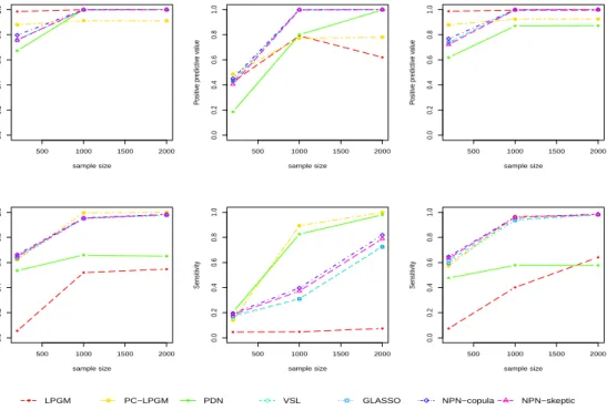
3.7 PPV (first panel row) and Se (second panel row) for PC-LPGM; LPGM; PDN; VSL; GLASSO; NPN-Copula; NPN-Skeptic for networks in Fig-ure 3.2 (p= 100), sample sizes n= 200, 1000, 2000 and λnoise = 0.5. . . . 49

3.8 PPV (first panel row) and Se (second panel row) for PC-LPGM; LPGM; PDN; VSL; GLASSO; NPN-Copula; NPN-Skeptic for networks in Fig-ure 3.2 (p= 100), sample sizes n= 200, 1000, 2000 and λnoise = 5. . . 49

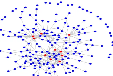
3.9 Distribution of four miRNA-Seq: raw data (top), normalized (bottom) data. . . 53 3.10 Breast cancer miRNA network estimated by the PC-LPGM algorithm

(hub nodes coloured red). . . 54 4.1 The graph structures for p= 10 employed in the simulation studies: (a)

scale-free; (b) hub; (c) random graph. . . 64 4.2 The graph structures for p= 100 employed in the simulation studies: (a)

scale-free; (b) hub; (c) random graph. . . 65

(14)

xii List of Tables 4.3 Number of TP edges recovered by PKBIC; PKAIC; Or-PPGM; Or-LPGM;

PDN; ODS; MMHC; K2mix; K2cut; PCmix; PClog for networks in Fig-ure 4.1 (p= 10) and sample sizes n = 200,1000,2000. . . 66 4.4 PPV (first panel row) and Se (second panel row) for PKBIC; PKAIC;

Or-PPGM; Or-LPGM; PDN; ODS; MMHC; K2mix; K2cut; PCmix; PClog for networks in Figure 4.1 (p= 10), sample sizes 200, 1000, 2000. . . 67 4.5 Number of TP edges recovered by PKBIC; Or-PPGM; Or-LPGM; PDN;

ODS; MMHC; K2mix; PClog for networks in Figure 4.2 (p = 100) and sample sizes n= 200, 1000, 2000. . . 68 4.6 PPV (first panel row) and Se (second panel row) for PKBIC; Or-PPGM;

Or-LPGM; PDN; ODS; MMHC; K2mix; PClog for networks in Figure 4.2 (p= 100), sample sizes n = 200,1000,2000. . . 69 5.1 An example of applying the PNS step on an undirected graph consisting

6 nodes. . . 75 5.2 An example of adding edge 3_→4 based on calculating the score matrix. 77 5.3 Number of TP edges recovered by plearnDAG; olearnDAG; llearnDAG;

PDN; ODS; MMHC; PClog for networks in Figure 4.1 (p = 10) and sample sizes n= 200, 1000, 2000. . . 80 5.4 PPV (first panel row) and Se (second panel row) for plearnDAG; olearnDAG;

llearnDAG; PDN; ODS; MMHC; PClog for networks in Figure 4.1 (p= 10), sample sizes n = 200, 1000, 2000. . . 81 5.5 Number of TP edges recovered by plearnDAG; olearnDAG; llearnDAG;

PDN; ODS; MMHC; PClog for networks in Figure 4.2 (p = 100) and sample sizes n= 200, 1000, 2000. . . 81 5.6 PPV (first panel row) and Se (second panel row) for plearnDAG; olearnDAG;

llearnDAG; PDN; ODS; MMHC; PClog for networks in Figure 4.2 (p= 100), sample sizes n= 200, 1000, 2000. . . 82

(15)

List of Tables

3.1 Monte Carlo marginal means of TP, FP, FN, PPV, Se obtained by sim-ulating 500 samples from each of the three networks shown in Figure 3.1 (p= 10). . . 50 3.2 Monte Carlo marginal means of TP, FP, FN, PPV, Se obtained by

sim-ulating 500 samples from each of the three networks shown in Figure 3.2 (p= 100). . . 51 4.1 Monte Carlo marginal means of TP, FP, FN, PPV, Se obtained by

sim-ulating 500 samples from random network with edge probability 0.03,

p= 100. . . 85 B.1 Simulation results from 500 replicates of the undirected graphs shown in

Figure 3.1 forp= 10 variables with Poisson node conditional distribution and level of noise λnoise = 0.5. Monte Carlo means (standard deviations)

are shown for TP, FP, FN, PPV and Se. . . 97 B.2 Simulation results from 500 replicates of the undirected graphs shown in

Figure 3.1 forp= 10 variables with Poisson node conditional distribution and level of noise λnoise = 5. Monte Carlo means (standard deviations)

are shown for TP, FP, FN, PPV and Se. . . 99 B.3 Simulation results from 500 replicates of the undirected graphs shown

in Figure 3.2 for p = 100 variables with Poisson node conditional dis-tribution and level of noise λnoise = 0.5. Monte Carlo means (standard

deviations) are shown for TP, FP, FN, PPV and Se. . . 100

(16)

xiv List of Tables B.4 Simulation results from 500 replicates of the undirected graphs shown

in Figure 3.2 for p = 100 variables with Poisson node conditional dis-tribution and level of noise λnoise = 5. Monte Carlo means (standard

deviations) are shown for TP, FP, FN, PPV and Se. . . 102 B.5 Simulation results from 500 replicates of the DAGs shown in Figure 4.1

for p = 10 variables with Poisson node conditional distribution. Monte Carlo means (standard deviations) are shown for TP, FP, FN, PPV and Se. . . 104 B.6 Simulation results from 500 replicates of the DAGs shown in Figure 4.2

for p= 100 variables with Poisson node conditional distribution. Monte Carlo means (standard deviations) are shown for TP, FP, FN, PPV and Se. . . 106 B.7 Simulation results from 500 replicates of the DAGs shown in Figure 4.1

for p = 10 variables with Poisson node conditional distribution. Monte Carlo means (standard deviations) are shown for TP, FP, FN, PPV and Se. . . 108 B.8 Simulation results from 500 replicates of the DAGs shown in Figure 4.2

for p= 100 variables with Poisson node conditional distribution. Monte Carlo means (standard deviations) are shown for TP, FP, FN, PPV and Se. . . 109

(17)

(18)

(19)

Introduction

Overview

Biological processes in a cell involve complex interactions between genes. These depen-dencies are commonly represented in the form of a graph. Indeed, graphs are transparent models, easily understood and used by researchers with very different backgrounds. As the direction of influence between genes is a crucial information, directed graphs are often used to represent such networks, a representation also particularly effective when it comes to deal with causal reasoning.

When the problem is to unravel which genes conditionally depend on each other, dependencies have to be inferred from experimental data. Graphical models, which powerfully represent complex multivariate distributions using the adjacency structure of a graph, are widely used to infer gene networks from experimental data. Learning a graphical model from the data boils down, statistically speaking, to making inference on the parameters of the multivariate distribution defined on the set of variables at hand. The state-of-the-art inference procedures assume that data arise from a multivariate Gaussian distribution. However, high-throughput omics data, such as those from next generation sequencing, often violate this assumption. Here, data are usually discrete, high dimensional, contain a limited number of samples, show a large number of zeros, and come from skewed distributions. A popular choice for adapting to non Gaussian data the large body of results available under the Gaussian assumption relies on data transformation. Indeed, some authors simply apply Gaussian graphical modelling to non Gaussian data after transforming the data by transformations such as log, Box-Cox, copulas, etc. This approach can work well in some circumstances. For example, microarray data are typically Gaussian on a log scale. Unfortunately, they can be also ill-suited, possibly leading to wrong inferences in some circumstances [Gallopin et al. (2013)]. This feeds the recent interest for new principled statistical procedures that can deal with different data distributions.

(20)

2 Overview The most natural idea relies on employing a joint multivariate distribution that, beside properly representing the set of relations among the variables, it respects the nature of the variables. A way to achieve this is to incrementally construct multivariate distributions through the specification of conditional distributions. Indeed, the so-called conditional modeling approach, is being recognized as an appealing approach to specify multivariate models that may contain complex dependence structures. Besag (1974) discussed a tractable and natural way to construct multivariate extensions of univari-ate exponential family distributions. The construction begins with specification of the conditional dependencies present among a finite set of random variables that result in a Markov random field. These conditional dependencies define which of the entries of the multivariate random vector can be considered as neighbours of each other. Various mod-els can then be constructed through specification of local (parametric, semiparametric, nonparametric) regression models.

In this thesis, we assume that conditional distributions follow a Poisson law (exten-sions to other count distributions could be obtained on the same lines) and we tackle structure learning of both undirected and directed acyclic graphs (DAGs). There are some results in the literature on structure learning of Poisson graphical models for undi-rected models [Allen and Liu (2013), Yang et al. (2013)], or directed graphical models that permit cycles on graphs [Hadiji et al.(2015)]. To the best of our knowledge, there is only one algorithm for structure learning of Poisson DAGs, i.e., Park and Raskutti (2015).

The outline of the thesis is as follows. In Chapter 1, we briefly review graphical mod-els and structure learning of graphical modmod-els. Poisson graphical modmod-els are introduced in Chapter 2. We address both the directed and the undirected framework, proposing a model specification proved to be identifiable. Some Poisson structure learning algo-rithms are also described. Chapter 3 presents our first proposal, aimed at learning the structure of undirected Poisson graphical models, provides a theoretical analysis of con-vergence of the algorithm and gives an empirical analysis of its performance. Chapter 4 covers the proposed solutions to guided algorithms. The key ingredient of guided structure learning is assuming that the topological ordering of the set of nodes is spec-ified beforehand. Three new algorithms for refining the graphical structure, i.e., PK2, Or-LPGM, Or-PPGM, are presented along with a theoretical analysis of convergence, and an empirical comparison with a number of different structure learning algorithms. In Chapter 5, we turn our attention to unguided structure learning. This is particularly relevant when the topological ordering may be misspecified, or only a partial ordering on the set of nodes is specified due to a number of reasons. We present the proposed

(21)

Introduction 3 algorithm, and give an empirical analysis of its performance. Chapter 6 contains main conclusions drawn from this project up to date and possible directions for future re-search.

Main contributions of the thesis

Main contributions of the thesis can be summarized as follows.

1. Definition of a supervised learning algorithm of undirected Poisson graphs, PC-LPGM. The algorithm stems from the local approach of Allen and Liu (2013), where the neighbourhood of each node is estimated in turn by solving a lasso penalized regression problem and the resulting local structures stitched together to form the global graph. To face possible inaccurate inferences when dealing with models of high dimension, we propose to substitute penalized estimation with a testing procedure on the parameters of the local regressions following the lines of the PC algorithm, see Spirtes et al. (2000). The PC-LPGM algorithm seems to be very appealing, since it inherits the potential of the PC algorithm that allows to estimate a sparse graph even if the number of nodes, i.e., p, is in the hundreds or thousands.

2. Definition of three partially supervised learning algorithms of DAGs, i.e., PK2, Or-LPGM, Or-PPGM, applicable in situations when some prior information per-taining to the topology of the graph is available. The methods are based on a modification of: a very popular structure learning algorithm, the so-called K2 algorithm [Cooper and Herskovits (1992)]; of the local Poisson graphical model (LPGM) [Allen and Liu (2013)]; of the PC algorithm [Spirtes et al. (2000)]. The main strength of these proposals is their simplicity and low computational cost, since exploiting knowledge of the ordering of the nodes allows to considerably reduce the search space.

3. Definition of a supervised learning algorithm of DAGs, learnDAG. We present an algorithm for learning the high dimensional Poisson DAGs, that can be generalized to the case with high variance. The main idea behind our proposal is based on estimating the “potential parent” sets from edge selection in a DAG by using a log likelihood score function. These potential parents are then taken as the input to a pruning step aimed to remove additional edges. Moreover, to make the algorithm feasible to deal with a high dimensional setting, we also include a preliminary neighbourhood selection to reduce dimensionality of the candidate neighbourhood

(22)

4 Main contributions of the thesis sets for each node. Results on experimental data show that this algorithm is quite promising in recovering the structure from given data alone.

4. Proof of identifiability of Poisson DAGs. We prove that assuming a Poisson node conditional distributions guarantees identifiability of DAG models.

5. Statistical guarantees (proofs of convergence are provided for most of the pro-posed algorithms) and extensive empirical studies of performance are given for all proposed algorithms.

(23)

Chapter 1 Background

In this chapter, we provide a brief introduction to graphical models. We will address both the directed and the undirected framework, including factorizations of probability distributions, their representations by graphs, and the Markov properties. In detail, we begin with the relation between conditional independence and graphs in Section 1.1. Some basic concepts on undirected graphical models, and directed graphical models are given in Sections 1.2, 1.3 respectively. In Section 1.5, we summarize three approaches of structure learning of graphical models.

1.1 Conditional independence and graphs

The set of conditional independences among a collection of random variables can be intuitively represented as relations defined on the sets of vertices of a graph induced by a certain separation criterion. This connection led Pearl and Paz (1985) to study conditional independence of variables with the help of graphs, where each variable cor-responds to a node, and edges of the graph encode the conditional dependences. This application of graphical methods gives rise to the so called graphical models.

In order to give an overview on graphical models, we start by giving the definition of conditional independence.

Definition 1.1.1. We say that random variablesX and Y are conditionally independent given the random variable Z and write X_⊥_⊥Y_|Z if and only if

P(X ∈A, Y ∈B|Z) = P(X ∈A|Z)P(Y ∈B|Z),

for any A and B measurable in the sample space of X and Y, respectively.

(24)

6 Section 1.1 - Conditional independence and graphs

X

Z

Y

Figure 1.1: An example of a conditional independence displayed graphically

Equivalently, we can say that the random variables X and Y are conditionally inde-pendent given the random variableZ if and only if_P(X _∈A_|Y, Z) = _P(X _∈A_|Z). This alternative definition has an intuitive interpretation: knowing Z renders Y irrelevant for predicting X. It is worth to note that unconditional independence can be seen as a special case of the above definition for Z trivial. However, the two conditions X_⊥_⊥Y, and X_⊥_⊥Y_|Z are very different and will typically not both hold unless we either have

X_⊥_⊥(Y, Z) or (X, Z)_⊥_⊥Y, i.e., if one of the variables is completely independent of both of the others. This fact is a simple form of what is known as Yule-Simpson paradox. For discrete variables, Definition 1.1.1 is equivalent to

P(X =x, Y =y|Z =z) =P(X =x|Z =z)P(Y =y|Z =z),

where the equality holds for all z such that _P(Z = z) > 0; whereas for continuous variables the requirement is

f(x, y_|z) =f(x_|z)f(y_|z),

where the equality holds almost surely. This conditional independence can be displayed graphically as in Figure 1.1. Some fundamental properties of conditional independence are listed bellow.

Proposition 1.1.2. For random variables X, Y, Z, and W it holds (C1) if X_⊥_⊥Y_|Z then Y _⊥_⊥X_|Z;

(C2) if X_⊥_⊥Y_|Z and U =g(Y), then X_⊥_⊥U_|Z; (C3) if X_⊥_⊥Y_|Z and U =g(Y), then X_⊥_⊥Y_|(Z, U);

(25)

Chapter 1 - Background 7 (C4) if X_⊥_⊥Y_|Z and X_⊥_⊥W_|(Y, Z), then X_⊥_⊥(Y, W)_|Z;

if density with respect to (w.r.t.) product measure f(x, y, z, w)>0 and (C5) if X_⊥_⊥Y_|(Z, W) and X_⊥_⊥Z_|(Y, W) then X_⊥_⊥(Y, Z)_|W.

Conditional independence can be seen as encoding abstract irrelevance. With the interpretation: knowing C, A is irrelevant for learning B, then (C1)₋ (C4) can be translated into:

(I1) if, knowing C, learning A is irrelevant for learning B, then B is irrelevant for learning A;

(I2) if, knowing C, learning A is irrelevant for learning B, then A is irrelevant for learning any part D of B;

(I3) if, knowingC, learningA is irrelevant for learningB, it remains irrelevant having learnt any part D of B;

(I4) if, knowingC, learningA is irrelevant for learningB and, having also learntA, D

remains irrelevant for learning B, then both ofA andDare irrelevant for learning

B.

The property analogous to (C5) is slightly more subtle and not generally obvious. More-over, the symmetry property (C1) is a special property of probabilistic conditional in-dependence, rather than that of general irrelevance.

We now recall some important definitions of independence models. LetV be a finite set. An independence model _⊥_⊥σ overV is a ternary relation over subsets of a finite set

V.

Definition 1.1.3 (Semi-graphoid). An independence model is a semi-graphoid if it holds for all subsets A, B, C, D:

(S1) symmetry, if A_⊥_⊥σ B|C then B⊥⊥σ A|C;

(S2) decomposition, if A_⊥_⊥σ (B∪D)|C then A⊥⊥σB|C and A⊥⊥σD|C;

(S3) weak union, if A_⊥_⊥σ (B∪D)|C then A⊥⊥σB|(C∪D);

(S4) contraction, if A_⊥_⊥σB|C and A⊥⊥σD|(B∪C), then A⊥⊥σ (B ∪D)|C.

Definition 1.1.4 (Graphoid). An independence model is a graphoid if it is a semi-graphoid and satisfies

(26)

8 Section 1.2 -Undirected Graphical Models Definition 1.1.5 (Compositional). An independence model is compositional if it satisfies (S6) composition, if A_⊥_⊥σB|C and A⊥⊥σD|C then A⊥⊥σ(B∪D)|C.

Note 1.1.6. The composition property ensures that pairwise conditional independence implies setwise conditional independence, i.e.,

A_⊥_⊥σB|C ⇔α⊥⊥σβ|C, ∀α∈A, β ∈B.

For a system V of labelled random variables Xv, v ∈ V, with distribution P we can

then define an independence model _⊥_⊥P by

A_⊥_⊥B_|C _⇔XA⊥⊥P XB|XC,

where XA = (Xv, v ∈ A) denotes the variables with labels in A. Obviously,

gen-eral properties of conditional independence (C1)₋(C4) imply that this independence model satisfies the semi-graphoid axioms, and the graphoid axioms if the joint density of the variables is strictly positive. An independence model of this kind is said to be probabilistic. We note that a probabilistic independence model is not compositional in general, however when P is a regular multivariate Gaussian distribution, then it is a compositional graphoid.

1.2 Undirected Graphical Models

In what follows, we consider ap-dimensional random vectorX= (X1, . . . , Xp) such that

(s.t.) each random variable Xs corresponds to a node of the graph G = (V, E) with

index set V =_{1,2, . . . , p_}. In an undirected graph G = (V, E), an edge between two nodes s and t, is denoted by (s, t). The neighbourhood of node s _∈V is defined to be the set N(s) consisting of all nodes connected to s, i.e., N(s) =_{t _∈V : (s, t)_∈ E_}. A path inG is a sequence of (at least two) distinct nodesj1, . . . , jn s.t. there is an edge

between jk and jk+1 , for all k ∈ {1,2, . . . , n}. A cycle is a path with the modification

that j1 =jn. If A⊂ V is a subset of a vertex set it induces a subgraph GA = (A, EA),

where EA ⊂ E is obtained from E so that only edges with both endpoints in A are

kept. A graph is complete if all its nodes are joined by an edge. A subset is complete if it induces a complete subgraph. A complete set that is maximal is called a clique.

(27)

Chapter 1 - Background 9

1.2.1 Separation in undirected graphs

Here, we recall an important concept of undirected graphs that represents the conditional independence of random variables, i.e., separation.

Definition 1.2.1 (Separation). LetG= (V, E) be finite and simple undirected graph (no self-loops, no multiple edges). For subsetsA, B, S ofV, we say that S separatesA from

B in G, and denoteA_⊥_⊥GB|S if all paths from A to B intersect S.

Note 1.2.2. It is easy to see that the separation relation on subsets ofV is a compositional graphoid; and the name “graphoid” for such separation relations also comes from this reason.

1.2.2 Markov properties on undirected graphs

We now review briefly three Markov properties associated with undirected graphs, see Lauritzen (1996) for a detailed presentation. Let XU = (Xj : j ∈ U ⊂ V) be the

random vector of all variables in U _⊂ V. The random vector X satisfies the pairwise Markov property w.r.t. Gif

Xs⊥⊥Xt|xV\{s,t},

whenever (s, t)_∈/ E. Moreover,X satisfies the local Markov property w.r.t. G if

Xs⊥⊥XV\{N(s)∪{s}}|xN(s),

for every node s_∈V. Finally, X satisfies the global Markov property w.r.t. G if XA⊥⊥XB|xC,

for any triple of pairwise disjoint subsets A, B, C _⊂ V such that C separates A and B

in G, i.e., every path between a node inA and a node in B contains a node in C. Note 1.2.3. For any semigraphoid it holds that the global Markov property implies the local Markov property, which in turn implies the pairwise Markov property. Although not true in general, the three Markov properties are equivalent when the independence relation on G satisfies graphoid axioms, that happens for example, when all variables

Xs, s ∈ V, are discrete with positive joint probabilities, or when X has a positive and

continuous density with respect to Lebesgue measure.

In an undirected graphical model, the pairwise Markov property infers a collection of full conditional independences encoded in absent edges. For this reason, performing

|V|

2

(28)

10 Section 1.3 - Directed Acyclic Graphical Models

G. The local Markov property means that every variable is conditionally independent of the remaining ones, given its neighbours. Hence, this property suggests that each variable Xs, s∈V, can be optimally predicted from its neighbour XN(s), giving rise to

the so called neighbourhood selection method. Under the global Markov property, one should look for separating sets to find conditional independence relations.

1.2.3 Factorization

Graphical models can also be defined in terms of density factorizations, as the joint dis-tribution can be expressed as a product of clique-wise compatibility functions. Consider a graph G = (V, E) with vertex set V = _{1, . . . , p_} corresponding to p variables and edge set E _⊂V _×V. Then, the definition of factorization is given as follows.

Definition 1.2.4 (Factorization). Suppose X = (X1, . . . , Xp) has a density w.r.t. a

product measure µ=_⊗p_s₌₁µs onR|V|, where µs is usually a Lebesgue measure if Xs is a

continuous random variable, or counting measure if Xs is discrete. LetC(G) be the set

of all complete subsets (cliques) of G, i.e.,C _{∈ C}(G) if (s, t)_∈E for all s, t_∈C. Then, the distribution of X is said to factorize according to Gif it has the density of the form

f(x) = Y

C∈G

φC(xC),

where the potential functionφC(.) is a function of|C|variables. Thus, a graphical model

can be defined by specifying families of potential functions.

Note 1.2.5. If f(.) factorizes, then it satisfies the global Markov property, as well as all weaker Markov properties (Hammersley and Clifford theorem), and, in the case of a graphoid, all the properties coincide.

1.3 Directed Acyclic Graphical Models

Consider ap-dimensional random vectorX= (X1, . . . , Xp) with index setV ={1,2, . . . , p}.

A directed graph _G = (V, E) is a structure consisting of a finite set V of vertices (also called nodes) and a finite set E of directed edges (also called arcs) between these ver-tices. A directed edge from nodek to nodej is denoted by (k, j) or k_→j, k is called a parent of node j, and j is a child of k. The set of parents of a vertex j, denoted pa(j), consists of all parents of node j, similarly for the set of children ch(j). If there is a directed path from k to j, then k is an ancestor of j and j is a descendant of k. The ancestors of j are an(j) and the descendants arede(k); similarly for sets of nodes Awe

(29)

Chapter 1 - Background 11 use an(A), and de(A). The non-descendants of a node k are nd(k) =V_\(_{k_{} ∪}de(k)). Two nodes that are connected by an edge are called adjacent. A triple of nodes (i, j, k) is an unshielded triple if i and j are adjacent to k but i and j are not adjacent. An unshielded triple (i, j, k) forms av-structure ifi_→k and j _→k. In this casek is called a collider. The skeleton of a graph Gis the set of all edges in G without direction, and denoted by ske(G).

Definition 1.3.1 (Partially directed acyclic graph). A graph is said to be a partially directed acyclic graph (PDAG) if there is no directed cycle, i.e., there is no pair (j, k) such that there are directed paths from j tok and from k to j.

Definition 1.3.2 (Directed acyclic graph). A directed acyclic graph (DAG) is a PDAG with all directed edges. In DAGs, a topological ordering j1, . . . , jp is an order ofpnodes

such that there are no directed paths from jk tojt if k > t for all k, t∈V.

Definition 1.3.3 (Topological ordering). A topological ordering of vertices of a directed acyclic graph is such that if a variable X is an ancestor of a variable Y in a graph G, then X precedes Y in that ordering.

Note 1.3.4. Obviously, such an ordering is generally non unique, but always exists.

1.3.1 Factorization

Using the locality defined by the parent-child relationship, the joint probability distri-bution can be factorized as the product of conditional densities.

Definition 1.3.5 (Factorization). Suppose X has a density with respect to a product measure. Then, the distribution of X factorizes according to a DAG G = (V, E) if it has a density of the form

f(x) = Y

j∈V

f(xj|xpa(j)),

where the f(xj|xpa(j)) are conditional densities with f(xj|x∅) = f(xj).

Note 1.3.6. We note that directed graphical models with directed cycles may not satisfy the factorization property.

1.3.2 d-connection/separation

In a DAG, independence is encoded by the relation of d-separation, defined below. Definition 1.3.7 (d-connection/separation). Two nodes j and k in V are d-connected given S _⊂V_\{j, k_} if G contains a pathπ with endpoints j and k s.t.

(30)

12 Section 1.3 - Directed Acyclic Graphical Models (ii) no non-collider on π is in S.

Generalizing to sets, two disjoint subsetsA, B _⊂V are d-connected givenS _⊂V_\(A_∪B) if there are two nodes j _∈A and k _∈B that are d-connected givenS. If this is not the case, then S d-separates A and B.

1.3.3 Markov properties on directed acyclic graphs

Similarly to what we have done for undirected graphs, we state the counterparts of Markov properties in DAGs.

A random vectorX= (Xv :v ∈V) satisfies the local Markov property w.r.t. a DAG

G if

Xv⊥⊥Xnd(v)\pa(v)|Xpa(v),

for every v _∈V . Similarly,X satisfies the global Markov property w.r.t. G if XA⊥⊥XB|XC

for all triples of pairwise disjoint subsets A, B, C _⊂V s.t. C d-separates Aand B inG, which we denote by A_⊥_⊥B_|C.

Note 1.3.8. It is always true for a DAG that the global property, local Markov property, and the factorization property are equivalent [Lauritzen et al. (1990)].

1.3.4 Moralization

A moral graph is a concept in graph theory, used to find the equivalent undirected form of a DAG.

Definition 1.3.9 (Moralization). The moral graph Gm of a DAGGis obtained by adding

undirected edges between unmarried parents and subsequently dropping directions. Note 1.3.10. If P factorizes w.r.t. G, then it factorizes w.r.t. the moralised graph Gm.

Hence, if P satisfies any of the directed Markov properties w.r.t. G, then it satisfies all Markov properties forGm. Moreover, it holds that A⊥⊥GB|S if and only ifS separates

A from B in this undirected graph Gm [Lauritzen (1996)].

1.3.5 Markov equivalent class

Every DAG determines a set of conditional independence relations among variables. It turns out that different directed graphs entail the same d-separation rules. These

(31)

Chapter 1 - Background 13 graphs are Markov equivalent and the set of Markov equivalent graphs is called a Markov equivalence class. The formal definition of Markov equivalence class is as follows: Definition 1.3.11 (Markov equivalence). Two graphs G1 and G2 are Markov equivalent

if their independence models coincide, i.e., if A_⊥_⊥G1 B|S ⇔A⊥⊥G2 B|S

Note 1.3.12. Two directed acyclic graphs G1 and G2 are Markov equivalent if and only if they have the same skeleton ske(G1) = ske(G2) and the same unshielded collider

tripaths.

The non uniqueness of the graphical representation has important practical conse-quences in statistical inference: in the problem of inferring the graphical structure from data, the underlying DAG is not identifiable, i.e., we cannot distinguish between DAGs in the same equivalence class. Hence, structure learning algorithms usually output an object representative of the whole equivalence class, the so called complete partially directed acyclic graph (CPDAG). A CPDAG is a graph that contains both directed and undirected edges. An edge between nodes i and j is directed in a CPDAG if and only if the orientation of that edge is the same across all DAGs in the equivalence class, otherwise we keep it undirected.

1.4 Faithfulness condition

The connection between graphs and probability distributions established by the concept of Markov property has been presented in Section 1.2 and Section 1.3 for undirected graphs and DAGs respectively. In particular, if there is a specific type of separation between nodes i and j of the graph given the node subset C then random variables Xi

and Xj are conditionally independent given the random vector XC in the probability

distribution. However, the “ultimate” connection between probability distributions and graphs requires the other direction to hold, namely for every conditional independence in the probability distribution to correspond to a separation in the graph. This connection has been called faithfulness of the probability distribution [Sadeghi (2017)].

Definition 1.4.1 (Faithfulness). A distribution _P is faithful to a graph G if no condi-tional independence relations other than the ones entailed by the Markov property are presented.

Note 1.4.2. LetJ(G) be the independence model induced by the graph G, andJ(_P) be the independence model induced by the distribution _P. Then, we say that _P is faithful to G if J(_P) =J(G).

The faithfulness condition holds in some cases, such as, for example, the Gaussian or the discrete case [Meek (1995)]. However, it does not hold in general.

(32)

14 Section 1.5 - Background on Structure Learning

1.5 Background on Structure Learning

When talking about learning in the graphical modelling framework, we distinguish two broad classes of problems: given a structure and a model specification, estimation of the model; and inferring the structure of the model from observation data. While the former is usually considered a traditional problem of statistical inference, the latter is usually covered in the machine learning literature. Here, we consider the latter problem, the so-called structure learning. In detail, given a set of observations that can be assumed to be independent and identically distributed (i.i.d.) instances sampled from a probability distribution_P corresponding to a graphG, we aim to recover the structure of the graph

G.

Structure learning algorithms can be roughly divided into two major approaches: scoring-based algorithms and constraint-based algorithms. Some hybrid algorithms are often defined mixing the two previous classes. The three approaches are touched upon in what follows. A description of some algorithms for continuous and categorical data is also provided in Appendix A, with special focus on the algorithms which we have used in our empirical studies.

1.5.1 Scoring-based Algorithms

Scoring-based algorithms make use of (i) a score function, such as, for example, the BIC score [Schwarz (1978)], the AIC score [Akaike (1974)], the Bayesian Dirichlet score [Heckerman et al. (1995)], the likelihood-equivalence Bayesian Dirichlet score [Heck-erman et al. (1995)], indicating how well the network fits the data; and (ii) a search strategy, which searches the model that maximizes the score in a possible structure space. We recall here the concept of consistency of a scoring criterion.

Definition 1.5.1 (Consistency of a scoring criterion). Assume that data are generated by some distribution_P∗whose underlying DAG isG∗(in other words, the set of conditional independence relations that hold in_P∗coincides with the set of conditional independence relations implied by G∗). We say that scoring function is consistent if the following properties hold as the number of observations goes to infinity, with probability that approaches 1:

i) the structure G∗ will maximize the score;

ii) all structures that are not equivalent to G∗ will have strictly lower score.

Especially when dealing with DAGs, the number of possible structures grows expo-nentially as a function of the number of nodes. For this reason, they often employ a

(33)

Chapter 1 - Background 15 greedy search, since searching over the space of possible networks is NP-hard. Chick-ering and Meek (2002) derived optimality results stating that the greedy search used in conjunction with any consistent scoring criterion will, as the number of observations goes to infinity, identify the true structure (up to an equivalence class).

1.5.2 Constraint-based Algorithms

Constraint-based algorithms make use of some statistical tests, such as, for example, the χ2 test of independence in contingency tables [Spirtes et al. (2000)], or the test on partial correlation under the Gaussian assumption [Kalisch and B¨uhlmann (2007)] to find conditional independence relations among the variables. When dealing with DAGs, an additional task needs to be considered, i.e., identifying the direction of edges on the graph. Here, the results of the conditional independent tests are used in conjunction with orientation rules to construct DAGs. This approach, in general, does not entail a unique graph when learning DAGs. As a consequence, results of constraint-based algorithms are often in the form of a CPDAG, i.e., an object representative of the whole equivalence class.

1.5.3 Hybrid Algorithms

Another class of methods, called hybrid methods, takes ideas from both the above de-scribed approaches. This approach is typically designed for learning DAGs. It usually works in two steps: firstly, conditional independence tests of the constraint based meth-ods are used to learn the skeleton of a the network; then, search-and-score methmeth-ods are performed over the graph structure space that respects the skeleton output to find the optimal structure. The resulting algorithms inherit advantages of both approaches. However, results of hybrid algorithms also suffer from disadvantages of both constraint-based algorithms and score-constraint-based algorithms, where algorithms require strong assump-tions and identify a graph up to Markov equivalence class.

(34)

(35)

Chapter 2 Poisson graphical models for count

data

In this chapter, we focus on Poisson graphical models. We address both the directed and the undirected framework, providing model specifications. As identifiability is an important issue of learning DAGs, we tackle identifiability of Poisson graphical models, proving that the proposed model specification leads to identifiable models. Some struc-ture learning algorithms are also described. In detail, Poisson model specification is given in Section 2.1. We prove that models are identifiable in Section 2.2. The Possion structure learning algorithms are reviewed in Section 2.3.

2.1 Model specifications

We will take a conditional approach as the starting point to model specification. In detail, assume that each conditional distribution of node Xs given a conditional set K

follows a Poisson distribution, i.e.,

Xs|xK ∼Pois(fs(xK)), (2.1)

where K is the set of neighbours of s, -denoted as N(s) in Poisson undirected graphs, -or the set of parents of s, -denoted as pa(s) in Poisson DAGs. The function fs(.) is an

arbitrary function representing the mean of the conditional distribution.

Different choices of the function fs(.) give rise to different model specifications. The

most usual choice for fs(.) is the link function of the univariate Poisson generalized

(36)

18 Section 2.1 -Model specifications linear models, i.e.,

fs(xK,θs) = exp{θs+ X t∈K θstxt}= exp{θs+ X t6=s θstxt}, (2.2)

whereθst = 0 ift /∈K, andθs={θs, θst, s∈V, t∈V\{s}}. Then, the node conditional

distribution is Pθs(xs|xK) = exp θsxs+ X t∈K θstxsxt−log(xs!)−eθs+ P t∈Kθstxt _,

where θs ∈ Θs ⊂ Rp. This specification defines an undirected graph G = (V, E) in

which one edge between node sand node timplies θst 6= 0 andθts 6= 0 (orfs(.) depends

onxt and ft(.) depends onxs). A missing edge between nodes and node t corresponds

to the condition θst = 0 or θts = 0 (or fs(.) does not depend on xt or ft(.) does not

depend on xs), implying conditional independence of Xs and Xt given the neighbours XK, i.e., Xs⊥⊥Xt|xK.

Similarly, in case of DAGs, the above specification puts an edge from nodes to node

t if θst 6= 0 (or fs(.) depends onxt). A missing edge s→t corresponds to the condition

θst = 0 (or fs(.) does not depend on xt), implying conditional independence of Xs and

Xt given the parents of s, i.e.,Xs⊥⊥Xt|xpa(s).

For DAGs, the joint distribution is easily obtained, since the joint distribution fac-torizes in terms of conditional distributions, leading to

Pθ(x) = p Y s=1 Pθs(xs|xpa(s)) (2.3) = exp p X s=1 θsxs+ X (s,t)∈E θstxsxt− p X s=1 log(xs!)− p X s=1 eθs+Pt∈pa(s)θstxt _. where θ =_{θs, s ∈V} ∈Θ⊂Rp×p. In case of undirected structures, if (and only if)

θst ≤0 ∀ s, t, the joint distribution over all random variables can be expressed in the

following symbolic form,

Pθ(x) = exp p X s=1 θsxs+ p X s=1 p X t=1 θstxsxt− p X s=1 log(xs!)−A(θ)}, (2.4)

whereA(θ) is a normalizing constant, see Allen and Liu (2013). In other words, a unique consistent joint distribution exists provided that conditional dependencies are all nega-tive, a condition also known as “competitive relationship” among variables, which highly

(37)

Chapter 2 - Poisson graphical models for count data 19 limits use of the distribution in applications. To overcome the above mentioned limi-tation, some authors suggest to modify base measures (or sufficient statistics) so as to guarantee the existence of a joint distribution allowing a richer dependence structure. The approach gives rise to the so called Truncated Poisson Graphical Models (TPGM), Quadratic Poisson Graphical Models (QPGM), and Sub-linear Poisson Graphical Mod-els (SPGM) [Yang et al. (2013)]. These three classes of graphical models permit rich dependence structures between variables, although they still have certain limitations on types of dependencies, or have a Gaussian-esque thin tail, or allow only a bounded range data.

But the question is if theoretical existence of a consistent joint distribution is required in real life applications, in particular when the interest is the structure of dependences. Indeed, some authors suggest to consider local conditional probability models regard-less of the existence of the joint distribution. In these cases, various models can be constructed through specification of local (parametric, semiparametric, nonparametric) regression models. These, combined with clever estimation solutions, give rise to a wide set of solutions able to embrace an extremely wide range of real situations. For exam-ple, to face sparsity of the graph, penalized regression techniques might be applied to estimate each conditional regression (see Allen and Liu (2013), Gallopin et al. (2013), ˇ

Zitnik and Zupan (2015)). A class of semiparametric models is proposed in Yang et al. (2014) along with an adaptive multistage convex relaxation algorithm to estimate pa-rameters in the model. The conditional mean could also be an arbitrary function, as in Hadiji et al. (2015).

2.2 Identifiability

An important issue of learning DAGs is the identifiability of the models. As stated before, different DAGs can encode the same set of conditional independences. Therefore, DAG models can be defined only up to their Markov equivalence class. However, in some cases, it is possible to identify the DAG by exploiting specific properties of the distribution, see Peters and B¨uhlmann (2013), Shimizu et al. (2006), Peters et al. (2012). Here, we prove that the Poisson DAG models in (2.3) are also identifiable.

It is worth remembering that an alternative proof of the identifiability of Poisson DAG models was also given in Park and Raskutti (2015). The Authors proved their result assuming a condition (Theorem 2.3.2, Section 2.3.3) which is in fact redundant in the setting under consideration. For this reason, we report here a detailed proof which benefits from the ideas developed in the work of Peters and B¨uhlmann (2013).

(38)

20 Section 2.2 - Identifiability Consider ap-random vectorX= (X1, . . . , Xp), and assume that the node conditional

distributions follow a Poisson distribution, i.e.,

Xs|xpa(s)∼Pois(exp{θs+

X

t∈pa(s)

θstxt}), s ∈V ={1, . . . , p}. (2.5)

For a fixed graphG, let paG(j), chG(j), and ndG(j) be the set of parents, the set of

children, and the set of non-descendants of node j inG, respectively.

Proposition 2.2.1. LetX be ap-random vector defined as in (2.5) and G= (V, E) be a DAG. Consider a variableXj, j∈V, and one of its parents k ∈paG(j). For all set S

with paG(j)\{k} ⊆S⊆ndG(j)\{k}, we have Xj⊥6⊥Xk|XS.

Proof. This proposition can be proved easily by using the definition of d-connection and the faithfulness assumption. Indeed, for a fixed node j _∈ V, for all k _∈paG(j) and for

all set S satisfies paG(j)\{k} ⊆ S ⊆ ndG(j)\{k}, there always exists the path k → j

satisfies the definition of d-connection. Hence, Xj ⊥6⊥Xk|XS.

Theorem 2.2.2. The Poisson DAG defined as in (2.5) is identifiable.

Proof. Assume there are two structure models as in (2.5) which both encode the same set of conditional independences, one with graph G, and the other with graph G0. We will show that G=G0.

Since DAGs do not contain any cycles, we can always find one node without any child. Indeed, assume to start at some node, and follow a directed path that contains the chosen node. After at most #(V ₋1) steps, a node without any child is reached. Eliminating such a node from the graph leads to a new DAG.

We repeat this process onG and G0 for all nodes that have: (i) no children, (ii) the same parents inGandG0. This process terminates with one of two possible outputs: (a) no nodes left; (b) a subset of variables, which we call againX, two sub-graphs, which we call againGand G0, and a nodej that has no children inGs.t. either paG(j)6=paG0(j)

or chG0(j)6= ∅. If (a) occurs, the two graphs are identical and the result is proved. In

what follows, we consider the case that (b) occurs. For such aj node, we have

Xj⊥⊥XV\(paG(j)∪{j})|XpaG(j), (2.6) thanks to the Markov properties with respect to G. To make our argument clear, we divide the set of parents paG(j) into three disjoint partitions W, Y, Z representing,

(39)

Chapter 2 - Poisson graphical models for count data 21 respectively, the set of common parents in both graphs; the set of parents in Gbeing a subset of children inG0; the set of parents inGwhich are not parents inG0. Formalizing,

• Z =paG(j)∩paG0(j);

• Y _⊂paG(j) s.t. chG0(j) =Y ∪T;

• W _⊂paG(j) s.t. W are not adjacent to j in G0.

Thus,

paG(j) = W ∪Y ∪Z, chG(j) = ∅,

paG0(j) = D∪Z, ch_G0(j) = T ∪Y,

whereDis not adjacent toj inG. LetU =W_∪Y and consider the following two cases:

• U =_∅. Then, there exists a node d_∈D or a node t_∈T, otherwise j would have been discarded.

– If there exists a noded _∈D, (2.6) impliesXj⊥⊥Xd|XQ, for Q=Z∪D\{d},

which contradicts Proposition (2.2.1) applied toG0.

– If D = _{∅}, and there exists a node t _∈ T, then (2.6) implies Xj ⊥⊥Xt|XQ,

forQ=Z_∪paG0(t)\{j}, which contradicts Proposition (2.2.1) applied to G0.

• U ₆=_∅. We note that, within the structure of the graphG0, the Poisson assumption implies Var Xj|Xpa_G0(j) =_E Xj|Xpa_G0(j) . (2.7)

(40)

22 Section 2.3 - Some Poisson structure learning algorithms Hence, from Equation (2.8), we get

Var Xj|Xpa_G0(j) = Var fj(XpaG(j))|XpaG0(j) +_{E E}(Xj|XpaG(j))|XpaG0(j) (2.9) = Var fj(XpaG(j))|XpaG0(j) +_{E E}(Xj|XpaG(j)∪XpaG0(j))|XpaG0(j) = Var fj(XpaG(j))|XpaG0(j) +_E Xj|Xpa_G0(j) ,

by applying (2.6). Equation (2.9) implies

Var Xj|XpaG0(j) >_E Xj|XpaG0(j) , since Var fj(XpaG(j))|XpaG0(j)

>0 in general, except at the root node.

2.3 Some Poisson structure learning algorithms

In this section, we briefly review three structure learning algorithms which make use of the Poisson assumption.

2.3.1 LPGM algorithm

The local Poisson graphical model (LPGM) algorithm is a scoring-based algorithm, designed to recover undirected Poisson graphical models. Introduced by Allen and Liu (2013), it assumes that the node conditional distributions follow a Poisson law, where the function fj(.) is taken to be the link function of the univariate Poisson generalized

linear models. It works by locally fitting a l1- penalized log-linear regression to each

node, i.e., to each random variableXs, given all other variablesXV\{s}as predictors. The

estimated graph is constructed as the union over the set of edges, found by employing the l1- penalized log-linear regressions.

In detail, letX(1)_{, . . . ,}_X(n) _be_n _independent_p_{-random vectors with the node}

condi-tional distribution specified in (2.1), whereX(i) _{= (}_X

i1, . . . , Xip); andX={x(1), . . . ,x(n)}

be the collection of n samples drawn from the random vectors X(1)_{, . . . ,}_X(n)_{, with}

x(i) _{= (}_x

i1, . . . , xip), i = 1, . . . , n. Let XU be the set of n samples of the |U|-random

vector XU, with x

(i)

U = (xij)j∈U, i= 1, . . . , n. Since we are only interested in

(41)

Chapter 2 - Poisson graphical models for count data 23 rewrite the node conditional distribution as follows

Xs|xV\{s} ∼Pois(exp{

X

t6=s

θstxt}), s∈V ={1, . . . , p}. (2.10)

Under the assumption (2.10), for each s _∈ V the node conditional distribution can be written as PθV\{s}(xs|xV\{s}) = exp{xs X t6=s θstxt−log(xs!)−e P t6=sθstxt_} _(2.11) = exp_{xshθV\{s},xV\{s}i+C(xs)−D(hθV\{s},xV\{s}i)},

where _h., ._i denotes the inner product,θV\{s} ={θst : t∈V\{s}}, C(a) = log(a!), a >

0, and D(a) = ea, a_∈_R.

Then, a rescaled negative node conditional log-likelihood is as follows

l(θV\{s},X) = − 1 n`(θV\{s},X) =− 1 nlog n Y i=1 PθV\{s}(xis|x (i) V\{s}) (2.12) = 1 n n X i=1 h −xishθV\{s},x(_Vi)_\{_s_}i+D(hθV\{s},x(_Vi)_\{_s_}i) i ,

where`(.) is the log-likelihood function. The parameter θV\{s} is estimated by

minimiz-ing the rescaled negative node conditional log-likelihood (2.12), i.e., ˆ

θV\{s} = argminθV\{s}∈Rp−1l(θV\{s},X). (2.13) To encourage sparsity of estimated graphs, a l1- regularized conditional log-likelihood is

considered, i.e., ˆ

θV\{s} = argminθV\{s}∈Rp−1l(θV\{s},X)−λkθV\{s}k1. Given the solution θˆV\{s}, the set of neighbours of node s is defined as

ˆ

N(s) =_{t _∈V_\{s_}: θˆst 6= 0}.

The regularization parameter λ that controls the sparsity of the graph structure is chosen by employing the stability selection criterion (StARS) as in Liu et al. (2010), which seeks the regularization parameterλleading to the most stable set of edges. More precisely, it considers a range Λ = _{λ1, . . . , λk} of values for λ, and fixes a number m,

(42)

24 Section 2.3 - Some Poisson structure learning algorithms generated from x1, . . . ,xn. For each λ ∈ Λ, the graph is estimated by solving a lasso

problem. Let Am

λ(S1), . . . , Amλ(SB) be estimated adjacency matrices of the graph in the

subsamples. The stability of one edge can be estimated by

m_s,t(λ) = 2ψ_s,tm(λ) 1₋ψ_s,tm(λ), whereψm s,t(λ) = 1 B PB

i=1Amλ(Si)st is the estimated probability of one edge between nodes

s and t. The optimal value λopt is defined as the largest value that maximizes the total

stability ¯ Dm(λ) =sup0≤ρ≤λ X s<t m_s,t(ρ)/ p 2 ,

smaller than a chosen value for the upper bound β, i.e., λopt = sup{λ : ¯DB(λ)≤β}.

2.3.2 PDN Algorithm

The Poisson dependency network (PDN) algorithm, introduced by Hadiji et al. (2015), is a nonparametric algorithm for structure learning of both directed and undirected Poisson graphical models. It is a scoring-based algorithm assuming that local conditional distributions follow a Poisson law, but fs(.) in (2.1) is set to be an arbitrary function.

Structure learning is achieved by estimating the mean function in a functional space, employing gradient ascent through gradient tree boosting, and multivariate gradient boosting.

Here, we consider two choices for the link function: log link function and identity function. For more comments on the choice of the link, we refer the interested reader to Hadiji et al.(2015).

For the log link function, we can rewrite the mean function as

fs(xV\{s}) = exp{ψs(xV\{s})},

where ψs(.) is some function of XV\{s}. In order to estimate ψ(xV\s), a gradient ascent

is applied in a function space for some iterations T,

(43)

Chapter 2 - Poisson graphical models for count data 25 where η, η > 0 is a step size parameter usually set equal to 1, and the function of gradient is: ∇t s = 1 n n X i=1 ∂ ∂ψt−1 s (x (i) V\{s}) log_P xis|x (i) V\{s};ψ t−1 s (x (i) V\{s}) = 1 n n X i=1 ∇t s(xis,x (i) V\{s}). The initial ψ0

s(xV\s) could be fixed to be constant or equal to the logarithm of the

empirical mean ¯xs or to a more complex model. This procedure gives a pointwise

estimate of fs(xV\{s}). However, the interest is in estimating fs(.) at arbitrary values x

other than those in the training sample. Hence, by imposing smoothness on the solution, the function estimate can be achieved by borrowing from nearby data points. One way to do it is using regression trees to approximate the true function gradient, i.e., the following objective is minimized

X j [ht_s(x(_Vi)_\{_s_})_{− ∇}t_s(xis,x (i) V\{s})] 2_, where ht

s(.) is a regression tree function as in Breiman et al. (1984). As some choices

can lead to really slow convergence, a multiplicative boosting approach with the use of identity link is employed.

For the identity link, i.e., fs(.) =ψs(.), the multiplicative update is specified by the

following theorem.

Theorem 2.3.1. The multiplicative functional gradient ascent using the identity link function is ψt+1(xV\{s}) = ψt(xV\{s})EXs,XV\{s} Xs fs(XV\{s})

and the training instance can be generated using

x(_Vi)_\{_s_}, xis fs(x (i) V\{s}) .

The main contribution of this method is the development of the multivariate gradient boosting, which is proved to be efficient in increasing the convergence rate, since it selects the step size automatically without extra computations.

2.3.3 ODS algorithm

The overdispersion score (ODS) algorithm, introduced in Park and Raskutti (2015), is one of the latest algorithms for learning large-scale Poisson DAGs. It belongs to the class of scoring-based algorithms and it works in two steps. Firstly, the topological ordering is estimated by using an overdispersion score function. Once the order is estimated, the

(44)

26 Section 2.3 - Some Poisson structure learning algorithms problem is reduced to an estimation ofpclassical penalized regression problems. Details of the ODS algorithm are given in what follows.

Similar to some other structure learning algorithms of DAGs that do not employ prior knowledge on topological ordering, ODS starts from searching the candidate par-ent sets by employing existing algorithms for learning undirected structures, such as, for example, those in Yanget al.(2012), Tsamardinoset al.(2006), or Aliferis et al.(2003). An estimated parent set is specified by learning a moral graph Gm _{= (}_{V, E}

u) underlying

the data. We recall that the moral graph of one DAG is defined as an undirected graph that consists of all edges on the original DAG without direction and edges between vari-ables that share a common child. Then, the algorithm estimates the (causal) ordering of Poisson DAGs using an overdispersion scoring criterion, which is based on this result: Theorem 2.3.2. Assume that for any j _∈V, K _⊂pa(j) and S _{⊂ {}1,2, . . . , p_}\K,

Var(fj(Xpa(j)|XS))>0.

Then Poisson DAG model is identifiable.

Precisely, the ordering begins from the node for which the difference between mean and variance is smallest. To identify the next position in the ordering, the j-th element is chosen from the neighbour set of (j₋1)-th element, for which the difference between conditional mean and variance on the intersection set between the (j₋1) first elements in the order and its neighbours reaches the minimum value. Once the topological ordering is known, the structure learning process boils down to pstandard regressions which can be performed by using traditional tools [Friedman et al. (2009)].

The score criterion of ODS exploits a simple property of Poisson DAGs, i.e, overdis-persion. However, it is also the drawback of this method, since it can not work on data which are not generated from a Poisson distribution.

(45)

Chapter 3 Structure Learning of undirected

graphs

This chapter intends to develop a framework for structure learning of undirected Poisson graphical models. We propose a new algorithm, called PC-LPGM, designed by exploiting two existing algorithms, i.e., the LPGM algorithm [Allen and Liu (2013)], and the PC algorithm [Spirtes et al. (2000)] (see Appendix A for details). Briefly, PC-LPGM employs the local approach of Allen and Liu (2013), i.e., it assumes, as PC-LPGM does, that each node conditional distribution follows a Poisson distribution. Then, the neighbourhood of each node is estimated in turn by a testing procedure on the parameters of the local regressions, following the lines of the PC algorithm.

The remainder of this chapter is as follows. Section 3.1 is devoted to the introduction of the proposed method, Section 3.2 provides a theoretical analysis of the algorithm with detailed proofs. In Section 3.3, we provide some experimental results that illustrate the practical performance of our method. Real data analysis on level III breast cancer miRNA expression is given in Section 3.4. Some discussion is provided in Section 3.5.

3.1 The PC-LPGM algorithm

We are considering the problem of learning an undirected (possibly sparse) graphical structure under model specification (2.10), i.e., each node conditional distribution fol-lows a Poisson distribution,

Xs|xV\{s} ∼Pois exp X t6=s θstxt , s_∈V =_{1, . . . , p_}. (3.1) 27

(46)

28 Section 3.1 - The PC-LPGM algorithm Structure learning can be performed by mean of conditional independence tests aimed at identifying the set of non-zero parameters θst. In the Poisson case, conditional

indepen-dencies can be inferred from Wald type tests on the parameters θst. Sample estimates

ˆ

θst can be obtained within a maximum likelihood approach and test statistics built

ex-ploiting the asymptotic normality of the estimators. It has to be said, however, that estimation might be problematic when the number of random variables p is large, pos-sibly larger than n. To face this problem, we borrow the solution offered by the PC algorithm, which relies on controlling the number of variables in the conditional sets, a strategy particularly effective when sparse graphs are under consideration.

Starting from the complete graph, for each s and t _∈ V_\{s_} and for any set of variables S_{⊂ {}1, . . . , p_}\{s, t_}, we test, at some pre-specified significance level, the null hypothesis H0 : θst|K = 0, with K = S∪ {t}. In other words, we test if data support

existence of the conditional independence relation Xs⊥⊥Xt|XS. If the null hypothesis

is not rejected, the edge (s, t) is considered to be absent from the graph. A control is operated on the cardinality of the setS of conditioning variables, which is progressively increased from 0 to p₋2 or to m, m < (p₋2), where m the maximum number of neighbours that one node is allowed to have.

In detail, assume Xs|xK ∼Pois exp X t∈K θst|Kxt , _∀s_∈V, K_{⊂ {}1, . . . , p_}\{s_}, (3.2)

and denoteθs|K ={θst|K : t ∈K}.A rescaled negative node conditional log-likelihood

given the conditioning variables XK ={Xk, k ∈K} can be written as

l(θs|K, X{s};XK) = − 1 nlog n Y i=1 Pθs|K(xis|x (i) K) (3.3) = 1 n n X i=1 h −xishθs|K,x (i) Ki+D(hθs|K,x (i) Ki) i ,

where the scaling factor is taken for later mathematical convenience. The estimate ˆθs|K

of the parameter θs|K is determined by minimizing the above given rescaled negative

conditional log-likelihood (3.3), i.e., ˆ

(47)

Chapter 3 - Structure Learning of undirected graphs for count data 29 A Wald-type test statistic for the hypothesis H0 : θst|K = 0 can be obtained from

asymptotic normality of ˆθs|K, i.e., from the result

√

n(ˆθs|K−θs|K)

d

−→N(0, I(θs|K)−1),

where I(θs|K) denotes the expected Fisher information matrix, i.e.,

I(θs|K) =E n∂ 2_l₍_θ s|K, Xs;XK) ∂2_θ s|K ,

which holds under fairly general regularity conditions. The test statistic for the null hy-pothesisH0 :θst|K = 0 can be obtained on exploiting the marginal asymptotic normality

of the component ˆθst|K.

In practice, the observed informationJ(θs|K) = n

∂2_l₍_θ

s|K,X{s};XK)

∂2_θ

s|K

, i.e., the second derivative of the negative log-likelihood function, is more conveniently used evaluated at ˆθs|K as variance estimate of maximum likelihood quantities instead of the expected

Fisher information matrix, a modification which comes from the use of an appropriately conditioned sampling distribution for the maximum likelihood estimators. Following this line, the test statistic for the hypothesis H0 :θst|K = 0 is given by

Zst|K = √ nθˆst|K r h J(ˆθs|K)−1 i tt , (3.5)

where [A]_jj denotes the element in position (j, j) of matrix A. It is readily available that Zst|K is asymptotically standard normally distributed under the null hypothesis,

provided that some general regularity conditions hold [Lehmann (1986), page 185]. The conditional independence tests are prone to mistakes. Moreover, incorrectly deleting or retaining an edge would result in changes in the neighbour sets of other nodes, as the graph is updated dynamically. Therefore, the resulting graph is dependent on the order in which the conditional independence tests are performed. To avoid this problem, we employ the solution in Colombo and Maathuis (2014), who developed a modification of the PC algorithm that removes the order-dependence, called PC-stable. In this modification, the neighbours of all nodes are searched for and kept unchanged at each particular cardinality lof the set K. As a result, an edge deletion at one level does not affect the conditioning sets of the other nodes, and thus the output is independent on the variable ordering.

Structure learning of graphs for count data

Structure Learning of Graphs for Count

Data

Abstract

Sommario

Acknowledgements

Contents

List of Figures

List of Tables

Introduction

Overview

Main contributions of the thesis

Chapter 1

Background

1.1

Conditional independence and graphs

1.2

Undirected Graphical Models

1.2.1

Separation in undirected graphs

1.2.2

Markov properties on undirected graphs

1.2.3

Factorization

1.3

Directed Acyclic Graphical Models

1.3.1

Factorization

1.3.2

d-connection/separation

1.3.3

Markov properties on directed acyclic graphs

1.3.4

Moralization

1.3.5

Markov equivalent class

1.4

Faithfulness condition

1.5

Background on Structure Learning

1.5.1

Scoring-based Algorithms

1.5.2

Constraint-based Algorithms

1.5.3

Hybrid Algorithms

Chapter 2

Poisson graphical models for count

data

2.1

Model specifications

2.2

Identifiability

2.3

Some Poisson structure learning algorithms

2.3.1

LPGM algorithm

2.3.2

PDN Algorithm

2.3.3

ODS algorithm

Chapter 3

Structure Learning of undirected

graphs

3.1

The PC-LPGM algorithm