TSE‐648
“Portfolio Selection in a Multi‐Input Multi‐Output Setting: a
Simple Monte‐Carlo‐FDH Algorithm”
Nicolas Nalpas,
Léopold Simar and Anne Vanhems
Portfolio Selection in a Multi-Input Multi-Output
Setting: a Simple Monte-Carlo-FDH Algorithm
Nicolas Nalpas
Toulouse Business School, University of Toulouse
L´eopold Simar∗
Anne Vanhems§
May 03, 2016
In memory of our friend Nicolas Nalpas, Professor at the Toulouse Business School, who died after a tragic accident on January 19th, 2015. He initiated and inspired this paper. Although we may not hope to close the void which he left behind, he and his work will live
on in ours.
Abstract
This paper proposes a nonparametric efficiency measurement approach for the static portfo-lio selection problem in a general inputs-outputs space, where inputs can include variance and kurtosis and outputs can include mean and skewness. Our work is in the vein of Briec, Kerstens and Jokung (2007) and Jurzenko, Maillet and Merlin (2006) who develop a directional dis-tance (shortage function) approach to evaluate the performance of portfolios in Mean-Variance-Skewness and in Mean-Variance-Mean-Variance-Skewness-Kurtosis spaces. Our approach use the Free Disposal Hull (FDH) estimator to derive an algorithm avoiding the heavy and non-robust numerical op-timization approaches suggested so far. This new approach is much faster, more robust to reach the optimum and more flexible since it can be extended to more general situations. We illustrate the algorithm with a data set on the French CAC 40 already used in the literature, to compare our method with the numerical optimization approaches.
Key Words: Directional Distance function, FDH estimator, Efficient frontier, Portfolio perfor-mance.
JEL Classification: G110; G120
∗Institut de statistique, biostatistique et sciences actuarielles, Universit´e catholique de Louvain, Voie du Roman
Pays 20, B1348 Louvain-la-Neuve, Belgium. Research supported by IAP Research Network P7/06 of the Belgian State (Belgian Science Policy).
1
Introduction
A large empirical literature has long and repeatedly documented the non-normality features of financial assets returns in numerous contexts like, among many others, stock returns in devel-oped (e.g., Harvey and Siddique, 2000 and Jondeau and Rockinger, 2003) and emerging (e.g., Chunhachinda et al., 1997) markets, exchange rates (e.g., Hsieh, 1989), hedge funds returns (e.g., Agarwal and Naik, 2004).
In particular, the return distributions of most financial assets exhibit strong asymmetry (non-null skewness) and fat tails (high kurtosis). In the meantime, several authors have shown that the portfolio selection based on the mean-variance criterion can entail a severe welfare loss in the presence of non-quadratic preferences and non-normally distributed asset returns (e.g., Jondeau and Rockinger, 2006 and Harvey et al., 2010). In such frameworks, mean-variance optimized portfolios appear to be suboptimal.
From a theoretical point of view, a decreasing absolute risk aversion together with a decreasing absolute prudence are sufficient conditions for which a risk-averse and non-satiable investor1 un-veils preferences with respect to portfolio higher-order moments in addition to mean and variance (Kimball, 1993). Typically, they are willing to accept lower expected return and higher volatility compared to the mean-variance benchmark in exchange for higher skewness and lower kurtosis (Horvath and Scott, 1980).
The main problem of extending the mean-variance framework to higher moments like skewness and kurtosis for portfolio selection is the difficulty to analyze the necessary trade-off between these four competing and conflicting objectives. As the dimensionality of the portfolio selection problem increases, it becomes difficult to develop a geometric interpretation of the quartic portfolio efficient frontier and to select the most preferred portfolio among boundary points.
Similarly as in the classical Markowitz framework, this problem has been tackled in the literature by the ways of either the use of Taylor series expansion (or somehow equivalently by a polynomial representation) of which order corresponds to the dimension of the problem under study to derive an approximation of the expected utility function to be maximized, or by solving a multi-dimensional optimization problem wherein investors exhibit preference (aversion) for odd (even) moments of the probability distribution of asset returns. None of these two approaches clearly dominate, each
1
These two attributes of investor preferences just mean that she is equipped with an increasing and concave utility function. These four properties of her utility function are considered as desirable (see Pratt, 1964; Arrow, 1970 and Kimball, 1993).
being subject to its own pitfalls.
Several criticisms can be addressed to the first approach in the portfolio choice context. Among others, examples of this approach can be found in Brandt et al. (2005), Dittmar (2002), Guidolin and Timmermann (2007), Harvey et al. (2010). The use of Taylor series expansion or polynomial representation may converge to the expected utility under restrictive conditions on the probability distribution of asset returns only. Moreover, there does not exist general rule for selecting the right order of truncation of these Taylor series expansions. In addition, the inclusion of an additional moment does not necessarily improve the quality of the approximation (see Brockett and Garven, 1998). Worse, optimal portfolios in this framework may not be feasible in practice. Finally, this approach intrinsically supposes the investor knows her utility function and preference parameters which lead to introduce a model risk.
The second approach assumes the existence of all considered higher moments of the probability distribution of asset returns and that they are relevant for the investor. In presence of skewness and kurtosis besides mean and variance, the characterization of the (Pareto) efficient frontier turns into a non-convex and non-smooth multi-objective optimization problem.
On a theoretical and partial point of view focusing on the variance at the expense of the two other criteria, Athayde and Flˆores (2004) provide an analytical solution characterizing the mean-variance-skewness (MVS) portfolio frontier by minimizing the variance subject to constraints on the mean and the skewness of the portfolio in the case where a risk-free asset exists and when short-sales are allowed. Empirically, the main issue relates to the existence of cubic (skewness) and quartic (kurtosis) objectives or constraints which make the optimization problem non-convex and potentially non-smooth.
To ensure the existence of a solution, most of the literature uses the so-called polynomial goal programming (PGP) approach which was originally introduced by Lai (1991) for selecting portfolios with some preference for skewness.2 In this two-step method, aspired levels regarding each decision criterion are first found independently from each other by solving as many optimization programs as the number of criteria considered. In the second step, a polynomial penalty function to be minimized is built using deviations from these optimal levels. A shortcoming of this approach relates to the connection between the exogenous parameters used to weigh the terms of the penalty function and the subjective investor’s preference regarding the selected moments of portfolio returns. Indeed,
2
Chunhachinda et al. (1997), Sun and Yan (2003) and Davies et al. (2009) are recent examples of the use of the PGP approach in a portfolio choice context which includes higher moments of asset returns.
several combinations of these paremeters can lead to nearly identical optimal portfolios. Moreover, only particular combinations together with specific formulations of the PGP when a risk-free asset exists and short sales are allowed may result in the selection of efficient portfolios in the space considered (see Briec et al., 2013).
To circumvent all these problems, recent promising approaches inspired by the non-parametric methods used in efficiency analysis and production theory has emerged. Contrary to the traditional methodology represented by the seminal work of Markowitz (1952), the efficient frontier is no longer computed point by point but characterized by projection from the original data set through non-linear forms of data envelopment analysis (DEA) models.3 Such techniques allow to evaluate the performance of a financial asset by measuring its distance with the optimal projection onto the efficient frontier. Morey and Morey (1999) propose two radial distances in a mean-variance (MV) framework and several time horizons. They consider successively an input orientation wherein they seek to minimize the variance without decreasing the expected return (the output of the model) and an output one in which the aim is to maximize the expected return without increasing the variance. Joro and Na (2006) extend this setting by including the skewness in an input-oriented model. These proposals rely on multiplicative measures of the distance and so require strictly positive inputs and/or outputs. This turns out to be critical when dealing with data containing zero or negative values as in financial databases. Such a restriction may strongly constraint the choice of inputs and outputs. Moreover, any oriented-radial measure of efficiency ignores the possibility that the investor looks for simultaneously increasing the output while reducing the input level of her investment.
Briec et al. (2004) and Briec et al. ( 2007) (hereafter BKJ) in a MV and a MVS setting respectively as well as Jurczenko et al. (2006) (hereafter JMM) where the kurtosis is also taken into account represent a step forward in this direction. All these non linear DEA-type models use a directional distance function (they use the term of shortage function) which looks simultaneously for reduction in inputs and expansion in outputs. For instance in a mean-variance-skewness-kurtosis (MVSK) framework, variance and kurtosis on one hand and expected return and skewness on the other hand are analogous to inputs and outputs in models of production. It then provides a perfect representation of the multi-dimensional choice set by locating any portfolio or fund relative to its projected point on the Pareto optimal efficient frontier. This boundary of the attainable set of
3
Standard linear DEA formulation results in overestimation of the variance, skewness and kurtosis of the projec-tion points because the diversificaprojec-tion effect is neglected.
assets gives a benchmark relative to which the efficiency of a fund can be measured. Despite the fact that when skewness and kurtosis are included into the analysis the efficient frontier turns out to be non convex, these authors provide a result which guarantees the global optimality of the projection on the boundary set.
Nevertheless, we argue that this result might not hold as soon as such models are implemented with standard optimization package. Using the same data set as in Briec et al. (2007), we show in the empirical section of this paper that, sometimes, such models cannot prevent from selecting only local optima. Even worse, we provide evidence that they may end up with unfeasible portfolios.
In this paper, we provide a method to overcome all these aforementioned drawbacks. We propose a fully non-parametric efficiency measurement approach for the static portfolio selection problem using the Free Disposal Hull (FDH) estimator and directional distances. The FDH approach allows to consider non-convex feasible sets, it has been originally proposed by Deprins et al. (1984) for multiplicative radial distances. Simar and Vanhems (2012) propose a simple method to extend the FDH estimator to the additive directional distances. The application of directional distance functions ensure the possibility of dealing with jointly negative inputs and outputs. Moreover this efficiency measure is invariant with respect to the unit of measurement which permits any kind of scaling. Our method allows to characterize the Pareto efficient set in a very general inputs-outputs space of any dimension. It only requires that these decision criteria must be defined by portfolio weights.
In our framework, the portfolio frontier is no longer numerically obtained through the resolution of a general non-convex optimization program but estimated thanks to a pure non-parametric statistical sampling approach, which allows to account for diversification effects. Because we do not rely to any sort of numerical optimization, our method is not subject to the computational limitations such as local optima which may arise when solving a nonlinear program. As far as we know, this is the first attempt to define a portfolio choice problem in such a way. This offers a large flexibility in the investor’s choice of inputs and outputs to be included in the analysis. The convergence of this estimated frontier towards the true one is also studied and is shown to be sufficiently fast to be implemented in practical contexts. Unlike in usual methods based on optimization, the complexity of our approach is kept at a minimum since it increases only linearly with the number of inputs and outputs in the problem.
The rest of the paper is organized as follows. In the next section, we present the foundation of our method in light with the existing literature on non-linear DEA models. Our statistical approach
and its properties together with the numerical algorithm to implement are discussed in the Section 3. Using the same data set as in BKJ and comparing our results with theirs, Section 4 provides an empirical illustration of the effectiveness of our approach in both a MVS and MVSK setting. Section 5 concludes.
2
Portfolio Selection in a general inputs/outputs space
2.1 Definitions and notations
We consider the problem of an investor selecting a portfolio among n risky assets. We assume a common practical situation wherein a risk-less asset is not available and no short-sales are allowed.4 It follows that the non-negative portfolio weightswmust sum to one, so belong to a simplex ofRn+. The investment opportunity set consists of all linear combinations of the ninitial (given) assets:
F ={w∈Rn+|w′in= 1
}
(2.1) where in is a vector (n×1) of ones.
The objectives, or investment criteria, of the investor can be split into two real vectors,x∈Rp
and y ∈ Rq, that respectively correspond to those to be minimized and those to be maximized. In production theory, they respectively relate to the inputs and the outputs of the activity under consideration. We can then define the set{(xi, yi)|i= 1, . . . , n}representing the inputs/outputs of
the original data set.
For a given portfolio, w ∈ F, we can then compute its inputs and outputs, (xw, yw),from the
previous set. Note that this characterizes the only restrictions in the choice of the inputs and outputs in our approach. In other words, it means that all the investor’s objectives, that can be considered, must be able to be calculated from a vector of portfolio weights. This framework is sufficiently general to handle a large set of investment criteria. It includes all those considered in the portfolio choice literature such as the moments or lower partial moments of any order of the distribution of asset returns, the portfolio beta, the value at risk and its conditional version, etc. So this covers the cases of Mean-Variance Skewness (MVS) and the Mean-Variance Skewness-Kurtosis (MVSK) settings of BKJ and JMM respectively.
4
The existence of a risk-free asset can easily be considered without loss of generality. Allowing the possibility of short selling should be studied carefully, since in such a case the set of feasible portfolios is no longer bounded. To keep this property, it would be possible, for instance, to constraint the portfolio expected return to be positive. We will not discuss any further such cases since they have much less practical implications.
Therefore, the inputs/outputs representation of the investment opportunity set, i.e. the port-folios generated by all possible linear combinations in F,is given by:
N ={(xw, yw)∈Rp+q|w∈ F
}
(2.2) As in BKJ and JMM, in order to identify the efficient frontier, namely the boundary ofN, we add a free disposability assumption regarding both the inputs and the outputs. This hypothesis simply states that it is always possible to achieve lower outputs with more inputs. The Free Disposal Hull (FDH) of N is then defined by:
Ψ = ∪ (xw,yw)∈N { (x, y)∈Rp+q |x≥xw, y ≤yw } (2.3) Note that this hypothesis does neither influence the search of optimal portfolios nor the measures of their efficiency (e.g., Lamb and Tee, 2012). This allows us to characterize the weakly efficient frontier as:
Ψ∂ ={(x, y)∈Ψ| for any (˜x,y˜) such that ˜x < x,y > y,˜ (˜x,y˜)∈/ Ψ} (2.4) It is worth noting that Ψ, the investment universe under the free disposability hypothesis, is not necessarily convex. It is obviously the case in a mean-variance framework when the sole input and output are respectively the expected return of the portfolio and its variance. In particular, we lose this convexity property in the MVS and MVSK setting.
From now on, we can characterize the efficient frontier using the very flexible approach based on directional distance functions introduced by Chambers et al. (1998). These functions ( called shortage functions in BKJ and JMM) generalize the traditional radial measures provided by both input and output distance functions. Given a direction vector (−gx, gy) where (gx, gy) ∈ Rp++q,
the directional distance function projects the input-output vector of a portfolio belonging to the feasible set, (x, y)∈Ψ, onto the efficient frontier in the chosen direction:
D(x, y;gx, gy) = sup{β|(x−βgx, y+βgy)∈Ψ} (2.5)
By definition, D(x, y;gx, gy) > 0 if and only if (x, y) ∈ Ψ. The set of points belonging to the
weakly efficient frontier, i.e. (x, y) ∈ Ψ∂, are characterized by D(x, y;gx, gy) = 0. Therefore, this
distance provides a direct measure of an asset efficiency along the direction, (gx, gy), towards which
we evaluate it. In particular, starting from an inefficient asset (x, y) such thatD(x, y;gx, gy)>0, it
reduce the inputs and expand the outputs to reach an efficient portfolio. The higher its value the more inefficient is the asset under consideration. Since this measure is additive, it allows to handle jointly any positive or negative values of inputs and outputs. This is highly desirable in financial applications where returns can obviously be negative.
This definition encompasses input or output radial distances as special cases, if g= (x,0) and
x >0 or g= (0, y) and y >0. Compared to these two traditional measures of efficiency, the main advantage of such a directional distance function comes from its properties of invariance: they are translation invariant and independent of unit of measurement when the units of the directional vectors are the same as the units of the inputs/outputs. Note that only the latter property is shared by traditional radial measures.
The translation property can be written asD(x−ηgx, y+ηgy;gx, gy) =D(x, y;gx, gy)−η,∀η∈R.
The unit free property of directional distance functions can be stated as follows: D(a.∗x, b.∗y;a.∗ gx, b.∗gy) =D(x, y;gx, gy),∀a∈ Rp+ and∀b ∈R
q
+, where.∗ denotes the component-wise product
between vectors. This property indicates that if units of measurement for inputs or outputs are changed, the corresponding direction vector must be rescaled to avoid changing the value of the directional distance function. This is particularly useful when the units of the components of x
and/or of y are quite different.
The choice of the direction vector along which to measure this directional distance appears really crucial as the former directly affects the latter. We will discuss in the next subsections how to incorporate investors preferences into the direction vector. But, let us discuss two particular selections in order to better interpret the meaning of the directional distance in such cases (e.g., F¨are
et al., 2008). On one hand, if the retained direction vector corresponds to the inputs/outputs of the problem, i.e. g= (gx, gy)≡(|x|,|y|), the directional distance function has a direct proportional
interpretation. It indicates by which proportion we need to simultaneously shrink the inputs and enhance the outputs to get an efficient portfolio. On the other hand, it can be also useful to work with normalized distances, using for instance the norm of the direction vector ∥g∥. This has the effect of scaling the directional distance function by the length of g. More explicitly, denoting
e
gx =gx/∥g∥and egy =gy/∥g∥, we have D(x, y;egx,egy) =
(
1/∥g∥)D(x, y;gx, gy). The advantage of
this measure comes from the fact that it directly gives the euclidean distance between (x, y) and its target on the efficient frontier, but the measure is no longer unit free.
Finally, as pointed in BKJ and JMM, the use of these directional distances can only guarantee the weak efficiency for a portfolio since it does not exclude projections on the vertical and horizontal
parts of the frontier of Ψ allowing for additional improvements.
2.2 Portfolio selection in MVS/MVSK spaces
The setting defined in the previous section is very general and flexible and can thus handle a large choice of inputs/outputs. We now particularize the formulation and the characterization of the efficient frontier in the MVS and MVSK spaces, following BKJ and JMM.
As stated in the previous subsection, we consider the problem of choosing a portfolio from the investor’s universe consisting of nrisky financial assets without the possibility of shorting. A portfolio is then represented by a vector of weights w= (w1, ..., wn) that belongs to her investment
universe defined in (2.1). Starting with the sample of historical returns, Rit,i= 1, ..., n, observed
over a period of time fromt= 1, ..., T, we can obtain the estimates of the first four moments by the following empirical counterparts for the (n×1) vector of meansE, the (n×n) variance-covariance matrixV, the (n2×n) skewness-coskewness matrix Sand the (n2×n2) kurtosis-cokurtosis matrix
K. Fori, j, k, ℓ= 1, . . . , n we have Ei= 1 T T ∑ t=1 Rit, Vij = 1 T T ∑ t=1 (Rit−Ei)(Rjt−Ej), Sijk= 1 T T ∑ t=1 (Rit−Ei)(Rjt−Ej)(Rkt−Ek), Kijkℓ= 1 T T ∑ t=1 (Rit−Ei)(Rjt−Ej)(Rkt−Ek)(Rℓt−Eℓ). (2.6)
Because of symmetries in these matrices, only a certain number of their elements need to be computed. When, as above, we consider a moment of orderκ= 1, ...,4, of then-dimensional vector of returns’ distribution, the number of distinct elements are given by
n−1 +κ
κ
. For instance, when we look at the(n2×n2)kurtosis-cokurtosis matrixK, only (n+3)(n+2)(n+1)n/24 elements must be calculated. If the investor has to choose a portfolio amongn= 35 financial assets, we just need to compute 73,815 elements and not 1,500,625.
To obtain the inputs/outputs representation of the investment opportunity set, as defined in (2.2), we need to classify the different goals of the investor in terms of inputs, i.e. objectives to minimize, and outputs, i.e. those to be maximized. As discussed in the introduction, investors express preference for odd moments and reluctance for even moments of the distribution of asset
returns. Therefore, when a MVSK framework is considered, we can define the set of inputs of the
n original assets asx1i =Vii; x2i =Kiiii and the set of outputs asy1i =Ei; y2i =Siii, whereas for
the MVS case, only the first input is considered.
The main innovation provided by BKJ and JMM for characterizing the efficient frontier Ψ∂ in such spaces is represented by the addition of the free disposability hypothesis as in (2.3). It allows to translate this multi-objective problem in just one optimization program instead of a multi-stage one as in the literature employing the PGP approach. Contrary to Morey and Morey (1999) and Joro and Na (2006) who utilize an input-oriented radial measure of efficiency, they both employ the more general and flexible directional distance function stated in (2.5).
Now, for any portfoliow∈ F, we have the following input-outputs correspondents
y1w =E(w) =w′E, (2.7)
x1w=V(w) =w′Vw, (2.8)
y2w =S(w) = (w⊗w)′Sw, (2.9)
x2w=K(w) = (w⊗w)′K(w⊗w), (2.10)
where ⊗denotes the Kronecker product. These relations provide the input/ouptut representation of the opportunity set in the MVSK case N = {(xw, yw)∈R4|w∈ F
}
, where of course we only consider the first input for the MVS setup. Note also that for the original assets, we have for
i= 1, . . . , n,x1i =x1ei, etc., where ei is the ith column of In, the identity matrix of ordern.
In the general formulation, using a specific direction vector g = (gx, gy) ∈ Rp++q, for an asset
(xw0, yw0), among the n to be evaluated, we have to solve in (w, β) the nonlinear maximization
problem
max
w∈F β
xw0 −βgx ≥xw
yw0 +βgy ≤yw (2.11)
where w0 is the corresponding column of the identity matrix for the original asset evaluated. The solution inβ give the efficiency of the asset (xw0, yw0).
the same without the second input K. For an asset (V(w0),K(w0),E(w0),S(w0)) we have max w∈F β V(w0)−βgV0 ≥V(w) K(w0)−βgK0 ≥K(w) E(w0) +βgE0 ≤E(w) S(w0) +βgS0 ≤S(w) (2.12)
For instance, and regarding the constraints defined over the inputs domain (first two constraints), they are two nonlinear constraints over the variance and the kurtosis objectives. In the right-hand side of the constraints, all possible combinations of portfolios returns expressed in terms of their mean, variance, skewness and kurtosis are considered and define all the feasible portfolios in the inputs/outputs space represented by Ψ as in (2.3), including the weakly efficient frontier defined in (2.4). The left-hand side of the constraints seeks proportionally to a factor β to, in the one hand, enhance the mean and skewness (the two constraints over the outputs domain) of the asset under evaluation, and in the other hand reduce its variance and kurtosis (the first two constraints over the inputs domain) in order to reach the efficient frontier along with the direction defined by the vector g= (gV0, gK0, gE0, gS0).
Let us denote (β∗, w∗) the optimal solution of the program (2.12). As discussed in Section 2.1, if we choose the direction gV0 =V(w0);gK0 =K(w0);gE0 =|E(w0)|and gS0 =|S(w0)|the distance β∗to the efficient frontier has a direct proportional interpretation. It indicates by which proportion we need to simultaneously shrink the inputs and augment the outputs to get an efficient portfolio.5 Accordingly, if β∗ = 0, the current asset (V(w0),K(w0),E(w0),S(w0)) is on the efficient boundary Ψ∂. Otherwise, it is inefficient and located below the boundary of Ψ, meaning that there exists a combinationw among the initial sample of assets that yields a higher mean and skewness together with a lower variance and kurtosis. The solution of the program (2.12) defines also the efficient projected point in the MVSK space, whose coordinates (V(w∗),K(w∗),E(w∗),S(w∗)).
Given the size n of the sample of assets, this program has to be runntimes, and we obtain n
efficiency measures and n projected portfolios onto the efficient frontier. They define the efficient frontier that is feasible in practice. To geometrically reconstruct the whole efficient frontier in such a space, two distinct procedures can be applied.The efficient frontier is uniquely defined by the
5
The absolute values are considered to avoid any possible negative values for the direction vector in both the mean and skewness dimensions.
boundary of the attainable set Ψ but the distance to the frontier, and so the resulting projected points, depends on the chosen direction. JMM proposes to run the program (2.12) by changing the direction vector as many times as needed. Another approach advocated by Kerstens et al. (2011) consists in building a point cloud representation by generating a large number of artificial assets, keeping their mean, variance, skewness and kurtosis in the range of values of the original data set. The efficient frontier is then obtained by replacing the original data points in the left-hand side of (2.12) and by solving the program as many times as the number of artificial assets. The solution points are obtained through the computation of the optimal values of the right-hand side of (2.12). It is also worth mentioning that the philosophy behind the BKJ’s or JMM’s approach is inspired by a non-linear form of Data Envelopment Analysis (DEA, Charnes et al., 1978). The traditional DEA is a linear model that constructs the efficient frontier either as a convex or as a linear (de-pending on model specifications) combination of the assets under evaluation. To account for the diversification effects in a portfolio choice context, thanks to the covariance, coskewness and cokur-tosis of asset returns, they adapt it by introducing the non-linearities in the right-hand side of the constraints of (2.12). Indeed, the variance, skewness and kurtosis of portfolio returns introduce respectively a quadratic, cubic and quartic constraint in the optimization program.
Therefore, whether in a MVS framework, or a MVSK one, each solution of (2.12) can only be obtained by solving a complex non-linear and non-convex optimization program. Only the restriction of the inputs/outputs space to linear (mean) and/or quadratic (variance) objectives can guarantee the convexity of Ψ. Since the objective function of such a non-linear optimization program is linear, local optima are also global in such cases. Using a similar proof, BKJ in a MVS space and JMM in a MVSK one provide a sufficient condition based on the free disposability showing that a local optimal solution of (2.12) is also a global optimum despite the non-convexity of Ψ in such frameworks.
Nevertheless, this theoretical result may not hold in practice when (2.12) is numerically solved using standard optimization packages. Indeed, since the program is non-linear and non-convex, it might be the case that the solution obtained corresponds only to a local optimal solution and not an absolute optimal, due to a bad choice of initial portfolio weights. Actually, a large number of algorithms proposed for solving non-convex problems are not capable of making a clear distinction between local optimal solutions and global optimal solutions, and will treat the former as actual solutions to the problem under consideration. Generally, global optimization solvers attempt to locate a global solution by repeating randomly the starting points. However, as far as we know, no
solver employs an algorithm that can certify a solution as global. We will come back to this point in Section 4 when we try to replicate BKJ results using the same data set.
As pointed above another flexibility of directional distances approaches is that is very convenient to introduce the preference of the investor by choosing appropriately the direction vector allowing to apply a desired weight to each variable; e.g. if the investor is as concerned by mean and variance but two times as less for skewness and kurtosis, he could choose the scaling factor (2,1,2,1) for the direction vector.
3
The Statistical Approach for Portfolio Selection
In this section we propose a simple algorithm that will avoid the numerical optimization programs. It will rather use nonparametric estimators of Ψ and their statistical properties to get a solution reaching the desired precision. The most natural nonparametric estimator of Ψ is the Free Disposal Hull (FDH) of a sample of portfolios. We first summarize its definition and present some properties which will be useful to describe our algorithm.
3.1 The FDH estimator and some basic properties
The starting point is the n observations (xi, yi), i = 1, . . . , n which are the portfolios we want
to evaluate. These define the original sample Xn. Suppose we generate N random weights wj,
j = 1, . . . , N over the space F. We can then build the N values of inputs and outputs XN =
{(xwj, ywj)|j = 1, . . . , N}, where (xwj, ywj) are computed from the weights wj and from the basic
data in Xn, according the transformations formulae given in (2.7). These generated portfolios can be viewed as a random sample ofN pairs (xj, yj) = (xwj, ywj)∈Ψ, where we simplify the notation,
but without ambiguity, the j index refering to a particular weight vector wj. Unless otherwise
stated we will in the sequel reserve the index i for the original data in Xn and we remind that (xi, yi) = (xei, yei) whereei is a weight vector being theith column ofIn. The free disposal hull of
XN provides the FDH estimator of Ψ corresponding to the N generated portfolios:
Ψ(XN) ={(x, y)|x≥xj, y ≤yj, j= 1, . . . , N}. (3.1)
It is the union of all the positive orthants in the inputs and of all the negative orthants in the outputs, whose origin coincides with the data points. This estimator was introduced in production efficiency analysis by Deprins et al. (1984), allowing non convex attainable sets. Its asymptotic
properties have been derived in Korostelev et al. (1995) and Park et al. (2000). Under mild regularity conditions, it has been shown that the rate of convergence of the resulting efficiency estimators is given by N1/(p+q). This means that the error of estimation when using the FDH estimator is of the order Op
(
N−1/(p+q))and it is there proven that the error converges at this rate to a limiting Weibull distribution.
A first useful fact of FDH estimator is that we do not need all the points inXN to characterize its free disposal hull. It is indeed clear, by definition of the FDH principle, that the free disposal hull of the FDH-frontier points of XN generates an identical set:
Ψ(XN)≡Ψ(XN∂) (3.2) whereXN∂ are the FDH-efficient points ofXN or equivalently, the set of undominated points inXN. This set may be defined as
X∂ N = { (xℓ, yℓ)∈ XN{(xj, yj)∈ XN|xj < xℓ, yj > yℓ}=∅ } .
Obviously the number of frontier points is given by N∂ = card(X∂
N)≤N.
The algorithm to compute the FDH estimator of the directional distances of any point (x, y) to the frontier of Ψ(XN) is very simple (see Simar and Vanhems, 2012) and based only on simple sorting algorithms, its complexity is linear in N :
b D(x, y;gx, gy; Ψ(XN∂)) = sup { β |(x−βgx, y+βgy)∈Ψ(XN∂) } , (3.3) where we explicit in our notation that the only needed data set is XN∂. Simar and Vanhems (2012) show that by a simple change of variable, a directional distance function can be viewed as a particular hyperbolic distance function in a transformed dataset. We can then benefit from the nice properties of directional efficiencies combined with simple tractable radial distance to compute appropriate estimators having known statistical properties. To simplify the notations we consider only the case where all the directions gx and gy are strictly positive. Daraio and Simar (2014)
explicitly show how to adapt the formulation and the notations to allow for directions containing some arguments equal to zero. This means that in a general setting, one could fix some sub-directions of inputs and/or outputs equal to zero whereas the attainable set is described in terms of the full dimensional space.6
6Note that in our application, the suggested directions by BKJ areg
x=|x|andgy=|y|, that we also use for ease
of comparison. So some elements may be equal to zero for some original data points inXn, for variables corresponding
The computation of the FDH-directional efficiency score of a given portfolio (x, y) relative to the sampleXN of theN generated portfolios can be summarized as follows. Consider the following transformation of the sample of frontier observations in XN:
˜
X∂
N ={(˜xℓ,y˜ℓ) = (exp(xℓ./gx),exp(yℓ./gy)) ;ℓ= 1, . . . , N∂} (3.4)
and consider also the transformed value (˜x,y˜) = (exp(x./gx),exp(y./gy)) of the point (x, y) under
evaluation. Then define JN as the set of the labels of observations in ˜XN∂ which dominate (˜x,y˜), which due to the monotonicity of the transformation is also given by the observations in XN∂ that dominate (x, y). It can be written as
JN ={j |(xj, yj)∈ XN∂, such thatxj ≤x, yj ≥y}. (3.5)
As explained in Simar and Vanhems (2012), the FDH directional distance estimator defined in (3.3) can then be easily computed with the following formula:
b D(x, y;gx, gy; Ψ(XN∂)) = log ( max j∈JN { min k=1,...,p, ℓ=1,...,q ( ˜ x(k) ˜ x(jk), ˜ y(jℓ) ˜ y(ℓ) )}) , (3.6) where for a vector a,a(k) denotes itskth component.
A second important fact is that this final value is determined by only one observation in the set
X∂
N of frontier points. We denote this particular point by (xref(x,y), yref(x,y)) where the label ref(x,y)
is the value of j ∈ JN giving the maximum when performing the max operation in (3.6). We call this point, the reference point of (x, y); it is a point inXN∂.
So to summarize, at any stage of the algorithm below once we have generated N random portfolios, the FDH-directional efficiency scores of the original units can be computed for all the original data points (xi, yi)∈ Xn, providing:
1. The nmeasures δi,N =Db(xi, yi;gx, gy; Ψ(XN∂));
2. N∂ points on the frontierXN∂ achieved at this stage; 3. The set of references points for the original assets:
X∂
ref ={(xℓ, yℓ), whereℓ= ref(xi,yi), i= 1, . . . , n} ⊆ X
∂
N. (3.7)
The latter reference set is by construction of cardinalitynref = card(Xref∂ )≤n, the inequality is due to the fact that a point in XN∂ can be the reference point of several original observations (xi, yi).
The error of the estimation isD(x, y;gx, gy; Ψ)−Db(x, y;gx, gy; Ψ(XN∂)) and optimally, we could
control this error by choosing N big enough by the convergence property of the FDH estimator, but in practice this would give a sample too big to handle in one shot, due to memory limitation of computers and the fact that many generated portfolios would be without interest, being far from the frontier. For instance, even in the simple Mean-Variance-Skewness case, p+q= 3 so to reach an error in estimating the directional distances of thenoriginal funds, of the order 10−3, we should need N ≈109.
The idea of the algorithm we suggest below is to reach such an objective, in an efficient iterative way. At each iteration k≥1 we will generateNcrandom weights to build new portfolios as convex
combinations of the useful portfolios retained at the end of iterationk−1. We adapt the procedure such that at each iteration the value of the achieved objective function in (3.3) cannot decrease while the number of random linear combinations used strictly increases. As we will see below, the algorithm is pretty fast and we achieve convergence to the global optimum in (2.5) even if the set Ψ is non convex.
3.2 The algorithm
During the process of the algorithm, we will generate, using random weights, Nc random convex
combinations of portfolios generated at the preceding step. We will keep at each step of the algorithm the characterization of the obtained portfolios in terms of a convex combinations of the
n original data points (xi, yi) in Xn. Indeed a convex combination of convex combinations of the
(xi, yi) remains a convex combination of the same points. The formula to build these new convex
combinations at each step is simply given by
Wk=Pk×Wk−1, (3.8)
where Wk−1 is a Nk−1 ×n matrix where each row is a weight vector wj ∈ F of the n original
funds coming from the preceding step, Pk is aNc×Nk−1 matrix, each rowpj being weights drawn
randomly from a Nk−1-dimensional unit simplex (
∑Nk−1
ℓ=1 pjℓ = 1 and pjℓ ≥ 0). We will discuss
below how to choose Nc and the matricesPk. 3.2.1 Initialization: step k= 0
The initial step of the algorithm is not so important but in practice the following choice has been shown to be rather efficient. At the very beginning we have only the n basic funds in Xn. We
first compute the FDH directional distances of the original funds: δi,n = Db(xi, yi;gx, gy; Ψ(Xn)).
Here again, Ψ(Xn)≡Ψ(Xn∂). Note that the frontier points have a weight matrix Wn∂ given by the corresponding rows of the identity matrix.
We then form all the n(n−1)/2 possible pairs of original funds giving equal weight to both elements of the pair, forming a n(n−1)/2×nmatrix of weights P0, each row having zero values
everywhere except in the 2 columns where we have the value 1/2, corresponding of the columns of the selected pair.7
The values of the inputs and outputs of these new portfolios are given by the basic transfor-mations in (2.7). For the full Mean-Variance-Skewness-Kurtosis cases, they are given element by element,j = 1, . . . , n(n−1)/2, by
x1(j) =w′(j)E
x2(j) = (w(j)⊗w(j))′Sw(j) y1(j) =w′(j)Vw(j)
y2(j) = (w(j)⊗w(j))′K(w(j)⊗w(j))
where w′(j) is the jth row ofP0 and E,V,S,Kare the return vector, and the variance-covariance,
skewness-coskewness and kurtosis-cokurtosis matrices of the original funds (given in (2.6)). We denote this set of portfolios Xc,0.
Now we form the starting data set asXinit =Xc,0∪Xn∂obtained by concatenating then(n−1)/2
equal weights combination with the original frontier points. This set of portfolios is characterized by the weighting matrix Winit = [P0′ Wn′∂]′. Of course we have here many inefficient portfolios,
so we identify the FDH frontier of this set, Xinit∂ and in particular, we can identify the reference points among them, as we did above in (3.7); this provides X∂
ref,0. We define N0 = card(Xref∂ ,0) as
the number of such points (remember we have N0 ≤n) and, in this initial step, this reference set will also be our starting set of frontier points, i.e. we define X∂
N0 =X
∂
ref,0. The corresponding rows
of the matrix Winit provides their weights WN∂
0 in terms of the original data (xi, yi); so W
∂ N0 is a N0×nweighting matrix.
An important element is that by construction Ψ(Xn∂)⊂Ψ(Xinit∂ ) so that the FDH-directional dis-tances of all thenoriginal funds at this stage given fori= 1, . . . , nbyδi,N0 =Db(xi, yi;gx, gy; Ψ(X
∂ N0)) =
b
D(xi, yi;gx, gy; Ψ(Xinit∂ )) are larger or equal to the basic original FDH values computed above
7
The choice of equal weights is motivated by the idea of not penalizing any initial funds at the beginning of the process.
δi,n =Db(xi, yi;gx, gy; Ψ(Xn∂)). We can appreciate the gain already obtained at this stage by
con-sidering, e.g., the Euclidean distance between the two vectors ∆0 = n ∑ i=1 ( δi,N0 −δi,n )2 .
The latter will be the criterion we will use to appreciate the convergence of the algorithm, although other measures (like e.g. maxi=1,...,n
(
δi,N0 −δi,n
)
could also be retained).
3.2.2 The iterations k≥1
Due to the notations introduced above, the algorithm is now easy to describe. We set k= 1. [1] Consider the setXMfof portfolios obtained by concatenating the efficient (frontier) portfolios
obtained at the preceding step with the original sample of n funds. We denote WMf the corresponding weights matrix. So we have
XMf= XN∂k−1 Xn with weightsWMf= WN∂k−1 Wn , (3.9) where of course Wn=In, the identity matrix.
[2] Now we draw randomly from these Mf = Nk−1 +n portfolios Nc pairs with two random
weights summing to one. The procedure is very robust to the choice ofNcand we could also
select more than 2 funds (we comment these issues below). The idea of reintroducing the original funds in the sample at each iteration avoids to penalize too quickly any original fund in the process associating to it a too low weight. This is achieved by building the matrix
Nc×Mf of weights Pk, each row of Pk now has zeros everywhere except for two random
weights summing to 1, in two randomly selected columns. As explained in (3.8) the set of these new generated portfolios have weights (in term of the initial funds (xi, yi)) given by
WM =Pk×WMf. By using these weights and similar formulae as in (2.6), we thus obtain the
set of points XM with inputsXM and and outputsYM.
[3] We now consider as current set of portfolios, the set obtained by concatenating XM just obtained above with the reference frontier points of the preceding step (k−1). This defines
XNk = XM ∪ X
∂
ref,k−1 . Adding the reference set of the preceding step is crucial to ensure
that Ψ(XNk−1)⊆Ψ(XNk) and so the FDH-directional distances of the original funds at step
k, can only increase:
δi,Nk =Db(xi, yi;gx, gy; Ψ(X
∂
Indeed taking the random convex combinations in step [2] above does not ensure this inequal-ity, because the reference points could disappear in the process.
[4] By computing theδi,Nkfori= 1, . . . , nwe have as byproduct the set of FDH frontier portfolios
at step k,XN∂
k and its reference subsetX
∂
ref,k that are ready to be used at the next iteration.
Of course tracing the appropriate rows of the weights matrix produces the matrix WN∂
k. We
can also compute the evaluation of the criterion ∆k = n ∑ i=1 ( δi,Nk−δi,n )2 ≥∆k−1, (3.11)
or any other similar.
[5] We now definek=k+ 1 and go back to step [1].
3.2.3 Stopping rule, convergence and tuning parameters
At each iteration k ≥ 1 we will generate Nc random weights to build new portfolios as convex
combinations of the useful portfolios retained at the end of iterationk−1. So, at the total we will analyze a sample ofkmax×Nc, just keeping at each iterations the pertinent (efficient and reference)
funds. Do to its statisyical convergence discussed above, the errors of the FDH estimators converge to zero when k increases. In addition, we have seen in (3.10), that we adapt the procedure such that at each iteration the value of the achieved objective function in (3.3) cannot decrease in the process. So we can either fix the total number of iterations kmax or define a stopping rule based
on the chosen criterion to appreciate the gain over the iterations. For instance we could stop when the relative increase of ∆k over the last 1000 iterations is less than 0.0001, or so.
We could define the complexity of the algorithm by the number kmax×Nc. The value of Nc
does not need to be big, because we will reiterate a large number of times. Small values ofNcallows
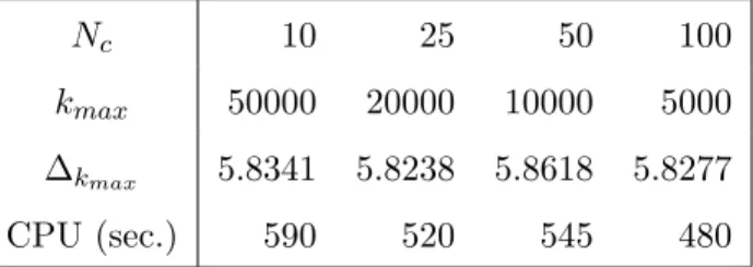
to speed up the process (random generation and the computation in each step) but will give less progress at each iteration. In our empirical illustration of the next section, we have n= 35 assets and we report in Table 3.2.3 some results for the full MVSK case to appreciate the sensitivity of the results to the choice of Nc; we see also the computing time for the fixed complexity of 50000.
We observe that globally the results are rather stable in terms of the achieved optimum (∆kmax),
but also in terms of computing time. In the empirical illustration below we will choose Nc = 50
Nc 10 25 50 100
kmax 50000 20000 10000 5000
∆kmax 5.8341 5.8238 5.8618 5.8277
CPU (sec.) 590 520 545 480
Table 1: Some results with “Complexity” = Nc ×kmax = 50000, n = 35, in the MVSK case. Computations are done on a Mac Book Pro, with processor 2,6 GHz Intel Core i5.
Finally, in step [2] of the algorithm, we generate random pairs (2 random weights). The process could also be done by drawingm≥2 random weights. The procedure is also robust to this choice, but the algorithm converges more quickly with the choicem= 2, probably because it give at each iteration more weight to the randomly selected portfolios.
4
Efficiency of Assets in the French CAC40
Just as an empirical illustration, we will compare the results obtained by out fast algorithm and those obtained by numerical optimization. We compute the efficiency of a small sample of n= 35 assets being part of the French CAC40 index between February 1997 and October 1999. This sample contains 567 daily returns Rit observations in common for all the assets. This data set is
the same as the one used by BKJ, where they only analyzed the MVS setup by using numerical optimization procedure (in GAUSS).8 So we will do the two analysis, the MVS and the MVSK. The moments are computed by using(2.6) providing the basic observations (xi, yi),i= 1, . . . , nbut
we keep the full matrices in order to compute by (2.7) the moments of any portfolio composition (w).
4.1 Analysis of our algorithm along the iterations
Before going into the comparison of the results, we first investigate how the algorithm behaves for the two cases along the iterations. As explained above, we have chosenNc= 50 andkmax= 10000.
Figure 1 represents the evolution of the solutions in the MVS case. In the left panel we see the values of ∆k, theL2 distances of the current FDH-directional distance at stepkwith thenoriginal
8
We acknowledge Chris Kerstens who was kind enough to provide us the data and the detailed results of their analysis in Briec et al. (2007).
values δi,n, before starting the algorithm. The right panel displays the evolution of the individual
efficiency scores δi,Nk. Figure 2 shows similar results for the MVSK case.
Figure 1: Evolution of the solutions through the MC iterations in the MVS case. Left panel, global criterion (L2 distances with original FDH values) and right panel, individual directional distances
for the 35 funds. Note that the relative increase in ∆k over the last 1000 iterations is 0.00028.
Iteration number 0 1000 2000 3000 4000 5000 6000 7000 8000 9000 10000 ∆k 1.5 2 2.5 3 3.5 4 4.5 5 Iteration number 0 1000 2000 3000 4000 5000 6000 7000 8000 9000 10000 δi,N k 0 0.1 0.2 0.3 0.4 0.5 0.6 0.7 0.8 0.9 1
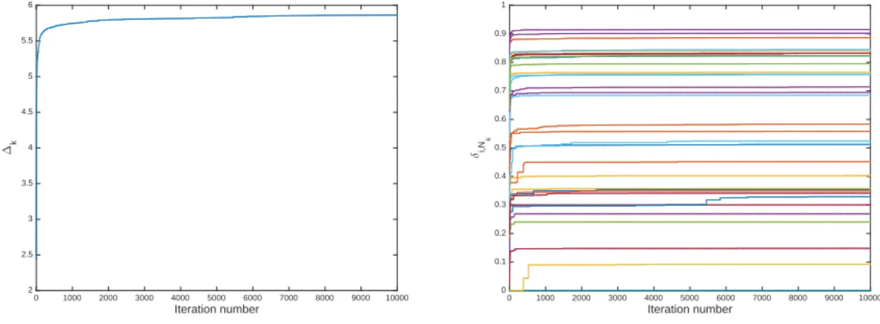
Figure 2: Evolution of the solutions through the MC iterations in the MVSK case. Left panel, global criterion (L2 distances with original FDH values) and right panel, individual directional distances for the 35 funds. Note that the relative increase in ∆k over the last 1000 iterations is 0.00026.
Iteration number 0 1000 2000 3000 4000 5000 6000 7000 8000 9000 10000 ∆k 2 2.5 3 3.5 4 4.5 5 5.5 6 Iteration number 0 1000 2000 3000 4000 5000 6000 7000 8000 9000 10000 δi,N k 0 0.1 0.2 0.3 0.4 0.5 0.6 0.7 0.8 0.9 1
We see on the figures that from k = 6000 (MVS case) and roughly k = 7000 (for the MVSK case) there is not much improvement left. Still for the MVS case, the relative improvement of ∆k over the last 1000 iterations was 0.00028 and for the MVSK case, 0.00026. It is interesting to
note that using a stopping rule based on a relative increase of the ∆k over the last 1000 iterations
smaller than 10−3, the algorithm stopped at iteration 5000 for the MVS case and at iteration 8000 for the MVSK case. The final results with these stopping rules were faster to obtain (by a factor given by the numbers of iterations) with almost the same final results as these presented in Table 2 (for MVS: 23 identical at 10−3, 7 with an increase of 10−3, 4 with an increase of 2∗10−3 and 1 with an increase of 3∗10−3; for the MVSK: 31 identical at 10−3, 4 with an increase of 10−3).
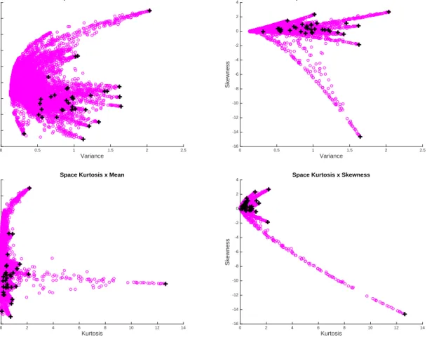
Figure 3 provides for the MVSK case, some 2-dimensional plots of 10000 random pairs portfolios builded by drawing pairs in the set of the final frontier points obtained at the end of our algorithm. The original n = 35 data points are also represented. This picture is only for illustrating how the Monte-Carlo principle works by drawing pairs at each iterations. Figure 4 provides the same picture in some 3-dimensional plots.
Figure 3: Some 2D plots of the cloud of 10.000 random pairs built portfolios, where the pairs are drawn in the set of the final frontier points augmented with the original 35 funds; the “circles” are the random pairs the “plus” are the original data.
Variance 0 0.5 1 1.5 2 2.5 Return -0.5 0 0.5 1 1.5 2 2.5 3 3.5
4 Space Variance x Mean
Variance 0 0.5 1 1.5 2 2.5 Skewness -16 -14 -12 -10 -8 -6 -4 -2 0 2
4 Space Variance x Skewness
Kurtosis 0 2 4 6 8 10 12 14 Return -0.5 0 0.5 1 1.5 2 2.5 3 3.5
4 Space Kurtosis x Mean
Kurtosis 0 2 4 6 8 10 12 14 Skewness -16 -14 -12 -10 -8 -6 -4 -2 0 2
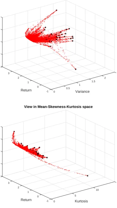
Figure 4: Some 3D plots of the cloud of 10.000 random pairs built portfolios, where the pairs are drawn in the set of the final frontier points augmented with the original 35 funds; the “small red points” are the random pairs the “black bullets” are the original data.
2.5 2
1.5
View in Mean-Variance-Skewness space
Variance 1 0.5 0 -1 0 Return 1 2 3 5 0 -5 -10 -15 4 Skewness 15 10
View in Mean-Skewness-Kurtosis space
Kurtosis 5 0 -1 0 Return 1 2 3 0 5 -15 -10 -5 4 Skewness
4.2 Detailed results and comparison with numerical procedures
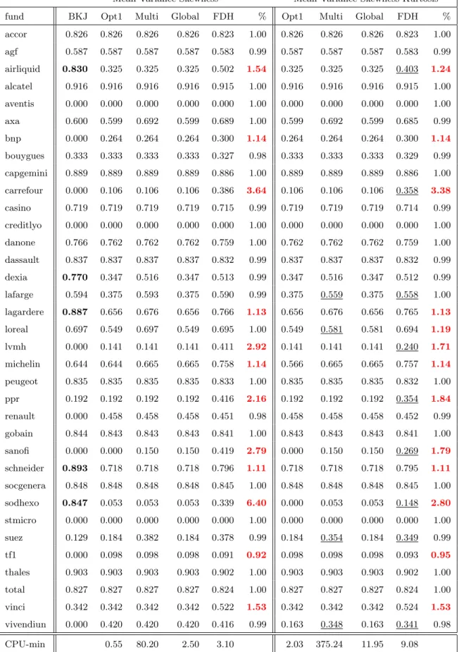
Now we can analyze our detailed results and the comparison with the results obtained by using numerical optimization. This is displayed in Table 2. The table has 11 columns of results, the first 6 are for the MVS case and the last 5 for the MVSK case. The column headed “BKJ” are the results coming form Briec et al. (2007) only for the MVS case. The columns “Opt1” gives the solution of numerical optimization using the fmincon (Matlab) procedure with only one starting value, as the one used by BKJ (wj = ej). The columns headed “Multi” use the Global Optimization Toolbox
from Matlab with the multistart option (we choose 100 different starting values generated by the procedure) and the columns “Global” uses the default global approach of the toolbox (roughly, 1000 random starting values are evaluated, among which the 200 best are kept but only a few ones, say 5, having the best score according some criterion (“basins of attraction”).9 The columns headed FDH are the results obtained by our iterative Monte-Carlo algorithm, already illustrated in the Figures 1 and 2. Finally the two columns headed “%” compare the best numerical procedure (given by the column “Multi”) with our FDH results: it is the ratio of the FDH-results divided by the Multi-results. A values bigger than 1 indicate better results with the FDH-Monte-Carlo method, in percentages (we used the convention % = 1 when we have 0/0).
This table deserves several comments.
1. In 2007, BKJ used a less performant optimizer than the ones available today. 5 of the results obtained (in bold) are far above the optimal values but it turns out that they are unfeasible (the constraints are not satisfied).10 We see also that 8 results are far below the optimal values including 7 assets wrongly stated as being efficient (β = 0) where they are not. The column “Opt1” indicates how today, using fmincon in Matlab, with the same starting values as in BKJ, we have better results, but still with some results far from the true optimum. This indicates that non-linear optimization is still in progress.
2. The use of the multistart options (with 100 different starting values) allows to obtain much better results, but at a computational cost (from 0.55 minute to 80,20 minutes). The Global option (with default tuning parameter) seems to be faster but not appropriate for the setup here. We will not comment the latter results in what follows but focus on the comparison between FDH and multistart.
9
See the user’s manual of the Global Optimization Toolbox of Matlab for more details.
10
3. Our algorithm (column FDH) is much faster (see the last row of the table: by a factor 25.9 = 80.2/3.1 for MVS and a factor 41.3 = 375.24/9.08 for MVSK) and as explained above with the automatic stopping rule it is even faster with almost identical results (by a factor 53.47, faster than multistart for MVS and a factor 56.68, for MVSK ).
4. The FDH results are generally much better than the multistart method. We see that in many cases our algorithm gives better solutions (the cases where % >1). For the MVS program, it is better in 11 cases (with a value of %=6.4), and only one slightly worse result for “tf1” with a measure FDH=0.091 in place of 0.098 obtained with the multistart algorithm. For the MVSK case, we observe 12 better results (with values as big as %=3.38) and only one worse result, again for “tf1” with an efficiency of 0.093, in place of the multistart value 0.098. This indicates that even with 100 different starting values, the numerical optimizers still stop at local optima in many cases, and with a much higher computational time.
5. As a consequence, the FDH approach is much more able to detect an effect of considering the Kurtosis, in addition to MVS. FDH detects substantial differences (δM V SK < δM V S) in
9 over the 35 cases (the underlined cases in the table). Note that the multistart procedure detects only 3 correct cases but reveals also a wrong effect (for “loreal”).
4.3 Conclusions of this illustration
The multistart procedure is certainly recommended when trying to solve the numerical optimization problems but still, we are never sure we end up with the true global optimum. In many cases, we are still on local minima. The FDH-Monte-Carlo algorithm we develop here seems to be much more robust, since it does not involves numerical optimization and there is no risk of being stucked on local minima. It is much faster and stable to the choice of tuning parameters of the algorithms. It is always easy to increase the number of iterations at a minimal computational cost.
Finally, we illustrated the algorithm in the MVS and MVSK cases, but it is very easy to adapt the procedure to any number of variables, as long as we can define these variables in terms of the weights of the portfolios (as for any moment), and it is also very easy to change the directions (for anlyzing the performances under different strategies). So our approach is certainly very flexible.
Mean-Variance-Skewness Mean-Variance-Skewness-Kurtosis fund BKJ Opt1 Multi Global FDH % Opt1 Multi Global FDH % accor 0.826 0.826 0.826 0.826 0.823 1.00 0.826 0.826 0.826 0.823 1.00 agf 0.587 0.587 0.587 0.587 0.583 0.99 0.587 0.587 0.587 0.583 0.99 airliquid 0.830 0.325 0.325 0.325 0.502 1.54 0.325 0.325 0.325 0.403 1.24 alcatel 0.916 0.916 0.916 0.916 0.915 1.00 0.916 0.916 0.916 0.915 1.00 aventis 0.000 0.000 0.000 0.000 0.000 1.00 0.000 0.000 0.000 0.000 1.00 axa 0.600 0.599 0.692 0.599 0.689 1.00 0.599 0.692 0.599 0.685 0.99 bnp 0.000 0.264 0.264 0.264 0.300 1.14 0.264 0.264 0.264 0.300 1.14 bouygues 0.333 0.333 0.333 0.333 0.327 0.98 0.333 0.333 0.333 0.329 0.99 capgemini 0.889 0.889 0.889 0.889 0.886 1.00 0.889 0.889 0.889 0.886 1.00 carrefour 0.000 0.106 0.106 0.106 0.386 3.64 0.106 0.106 0.106 0.358 3.38 casino 0.719 0.719 0.719 0.719 0.715 0.99 0.719 0.719 0.719 0.714 0.99 creditlyo 0.000 0.000 0.000 0.000 0.000 1.00 0.000 0.000 0.000 0.000 1.00 danone 0.766 0.762 0.762 0.762 0.759 1.00 0.762 0.762 0.762 0.759 1.00 dassault 0.837 0.837 0.837 0.837 0.832 0.99 0.837 0.837 0.837 0.832 0.99 dexia 0.770 0.347 0.516 0.347 0.513 0.99 0.347 0.516 0.347 0.512 0.99 lafarge 0.594 0.375 0.593 0.375 0.590 0.99 0.375 0.559 0.375 0.558 1.00 lagardere 0.887 0.656 0.676 0.656 0.766 1.13 0.656 0.676 0.656 0.765 1.13 loreal 0.697 0.549 0.697 0.549 0.695 1.00 0.549 0.581 0.581 0.694 1.19 lvmh 0.000 0.141 0.141 0.141 0.411 2.92 0.141 0.141 0.141 0.240 1.71 michelin 0.644 0.644 0.665 0.665 0.758 1.14 0.566 0.665 0.665 0.757 1.14 peugeot 0.835 0.835 0.835 0.835 0.833 1.00 0.835 0.835 0.835 0.832 1.00 ppr 0.192 0.192 0.192 0.192 0.416 2.16 0.192 0.192 0.192 0.354 1.84 renault 0.000 0.458 0.458 0.458 0.451 0.98 0.458 0.458 0.458 0.452 0.99 gobain 0.844 0.843 0.843 0.843 0.841 1.00 0.843 0.843 0.843 0.841 1.00 sanofi 0.000 0.000 0.150 0.150 0.419 2.79 0.000 0.150 0.150 0.269 1.79 schneider 0.893 0.718 0.718 0.718 0.796 1.11 0.718 0.718 0.718 0.795 1.11 socgenera 0.848 0.848 0.848 0.848 0.845 1.00 0.848 0.848 0.848 0.845 1.00 sodhexo 0.847 0.053 0.053 0.053 0.339 6.40 0.000 0.053 0.053 0.148 2.80 stmicro 0.000 0.000 0.000 0.000 0.000 1.00 0.000 0.000 0.000 0.000 1.00 suez 0.129 0.184 0.382 0.184 0.378 0.99 0.184 0.354 0.184 0.349 0.99 tf1 0.000 0.098 0.098 0.098 0.091 0.92 0.098 0.098 0.098 0.093 0.95 thales 0.903 0.903 0.903 0.903 0.902 1.00 0.903 0.903 0.903 0.902 1.00 total 0.827 0.827 0.827 0.827 0.824 1.00 0.827 0.827 0.827 0.824 1.00 vinci 0.342 0.342 0.342 0.342 0.522 1.53 0.342 0.342 0.342 0.524 1.53 vivendiun 0.000 0.420 0.420 0.420 0.416 0.99 0.163 0.348 0.163 0.341 0.98 CPU-min 0.55 80.20 2.50 3.10 2.03 375.24 11.95 9.08
5
Conclusion
In this paper we address the problem of portfolio selection in a multi-input multi-output setup. An example of that is when we want to minimize variance and kurtosis (inputs) and maximize mean return and skewness (outputs). One popular way to address these multi-criteria problem is based on directional distance (or shortage functions) in the lines of Briec et al. (2007) and Jurzenko et al. (2006). When using such higher order moments, the mathematical optimization problem results in highly nonlinear and difficult problems to handle: too often the numerical algorithms end up with local optima. We propose a very simple Monte-Carlo-FDH approach which avoids these numerical difficulties. It is based on a statistical approach of the problem generating appropriate random portfolios and estimating the non-convex efficient frontier with the FDH estimator. This approach turns to be faster with a better precision of the results and robust to numerical accidents.
In addition our new approach is very flexible (allowing the change the weights of the directional vector to reflect some other strategies of the investor) but also allowing to handle any kind of inputs and outputs (like other higher moments or function of these) as long as we can easily describe the decision criteria in terms of the portfolio weights.
We illustrate how our approach works in a data set on the French CAC 40 already used in the literature for the Mean-Variance-Skewness and the Mean-Variance-Skewness-Kurtosis setups and compare it with the disappointing results obtained by using the traditional numerical optimization techniques.
Since our approach is put in a statistical framework, further research may include testing the relevance of certain inputs and outputs and analyzing the sensitivity of the efficiency measures to the random nature of the basic data (empirical moments).
References
[1] Agarwal, V., N. Naik. 2004. Risks and Portfolio Decisions Involving Hedge Funds. Review of Financial Studies 17 63-98.
[2] Arrow, Kenneth J. 1970. New Ideas in Pure Theory: Discussion. American Economic Review 60(2) 462-63.
[3] Athayde, G., R. Flˆore. 2004. Finding a Maximum Skewness Portfolio a General Solution to Three-moments Portfolio Choice. Journal of Economic Dynamics and Control 28 1335-1352. [4] Brandt, M. W., Goyal, A., Santa-Clara, P., J. R. Stroud. 2005. A simulation approach to
dynamic portfolio choice with an application to learning about return predictability. Review of Financial Studies 18(3) 831-873.
[5] Briec, W., Kerstens, K., J.B. Lesourd. 2004. Single-Period Markowitz Portfolio Selection, Per-formance Gauging and Duality: a Variation on the Luenberger Shortage Function. Journal of Optimization Theory and Applications 120 1-27.
[6] Briec, W., Kerstens, K., O. Jokung. 2007. Mean-Variance-Skewness Portfolio Performance Gauging: A General Shortage Function and Dual Approach. Management Science 53 135-149. [7] Briec, W., Kerstens, K., Van de Woestyne, I. 2013. Portfolio selection with skewness: A compar-ison of methods and a generalized one fund result. European Journal of Operational Research 230(2) 412-421.
[8] Brockett, P. L., Garven, J. R. 1998. A reexamination of the relationship between preferences and moment orderings by rational risk-averse investors. The Geneva Papers on Risk and Insurance Theory 23(2) 127-137.
[9] Chamberlain, G. 1983. A characterization of the distributions that imply mean-variance utility functions. Journal of Economic Theory 29 185-201.
[10] Chambers, R.G., Y.H. Chung, R. F¨are. 1998. Profit, Directional Distance Functions and Nerlo-vian Efficiency. Journal of Optimization Theory and Applications 98 351-364.
[11] Charnes, A., Cooper, W.W., Rhodes, E. 1978. Measuring the efficiency of decision making units. European Journal of Operational Research 2 429444.
[12] Chunhachinda, P., K. Dandapani, S. Hamid, A.J. Prakash. 1997. Portfolio Selection and Skew-ness: Evidence from International Stock Markets. Journal of Banking and Finance 21 143-167. [13] Daraio, C., L. Simar. 2014. Directional Distances and their Robust Versions: Computational
and Testing Issues. European Journal of Operational Research 237 358-369.
[14] Davies, R., H. Kat, S. Lu. 2009. Fund of Hedge Funds Portfolio Selection: A Multiple-Objective Approach. Journal of Derivatives and Hedge Funds 15(2) 91-115.