INFORMATION TO USERS
This manuscript has been reproduced from the microfilm master. UMI films the text directly from the original or copy submitted. Thus, some thesis and dissertation copies are in typewriter face, while others may be from any type of computer printer.
The quality o f th is rep ro d u ctio n is d ep en d e n t upon the quality of th e copy subm itted. Broken or indistinct print, colored or poor quality illustrations and photographs, print bleedthrough, substandard margins, and improper alignment can adversely affect reproduction.
In the unlikely event that the author did not send UMI a complete manuscript and there are missing pages, th ese will be noted. Also, if unauthorized copyright material had to be removed, a note will indicate the deletion.
Oversize materials (e.g., maps, drawings, charts) are reproduced by sectioning the original, beginning a t the upper left-hand comer and continuing from left to right in equal sections with small overlaps.
ProQ uest Information and Learning
300 North Zeeb Road, Ann Arbor, Ml 48106-1346 USA 800-521-0600
UNIVERSITY OF OKLAHOMA GRADUATE COLLEGE
BRIDGE WEIGH-IN-MOTION (WIM) ALGORITHM FOR
ESTIMATING AXLE WEIGHTS, AXLE SPACING, AND OTHER
TRUCK PARAMETERS
A Dissertation
SUBMITTED TO THE GRADUATE FACULTY in partial fuifilimcnt o f the requirements for the
degree of
DOCTOR OF PHILOSOPHY
By
SARAH K.LEM ING Norman, Oklahoma
UMI Number: 3073701
UMI*
UMI Microform 3073701
Copyright 2003 by ProQuest Information and Learning Company. All rights reserved. This microform edition is protected against
unauthorized copying under Title 17, United States Code. ProQuest Information and teaming Company
300 North Zeeb Road P.O. 60x1346 Ann Arbor, Ml 48106-1346
© Copyright by SARAH K. LEMING 2002 Ail Rights Reserved
BRIDGE WEIGH-IN-MOTION (WIM) ALGORITHM FOR ESTIMATING AXLE WEIGHTS, AXLE SPACING, AND OTHER TRUCK PARAMETERS
A Dissertation APPROVED FOR THE
SCHOOL OF AEROPSACE AND MECHANICAL ENGINEERING
BY
Dr. Harold S ta lfo i^(Committee Chair)
Dr. Charles Bert
Chang
Table of Contents
Table o f Contents...iv
List o f Figures...viii
List o f T ables...xiv
A bstract...xviii
1. WIM Systems and Force Identification M ethods...1
1.1 In-Service WIM System s... 3
1.2 Force Identification M ethods...9
2. Bridge M odels...16
2.1 Combination M odels...17
2.2 Multiple Beam M odels... 20
2.3 Single Beam M odels... 21
2.4 My M odels... 22
2.5 Static B eam ... 24
2.6 Finite Element M o d el... 24
2.7 Solution o f the Differential Equation... 26
2.8 Static Beam Bending Equation...27
2.9 Dynamic B eam ... 28
2.10 R(s^) ...31
2.11 Reduced Order M o d el... 32
2.12 Sensor Location...34
2.13 Chapter Conclusions... 37
3. Truck M odels...41
3.1 3D Truck M odels... 43
3.2 2D Truck M odels... 44
3.3 ID Truck M odels... 46
3.4 Static W eight...52
3.5 Numerical Parameters Used in Static Truck M odels...52
3.6 Numerical Parameters Used in Dynamic Truck M odels... 53
4. Bridge/Truck Interaction... 56
4.1 Iterative Solutions... 56
4.2 Other M ethods...57
4.3 Direct Integration... 57
4.4 Truck Crossing the B ridge...58
4.5 Static Bridge/Static T ru ck ...60
4.6 Static Bridge/Dynamic T ru ck ... 61
4.7 Dynamic Bridge/Static T ruck... 64
4.8 Dynamic Bridge/Dynamic T ruck... 65
5. Optimization and Problem Statem ent... 68
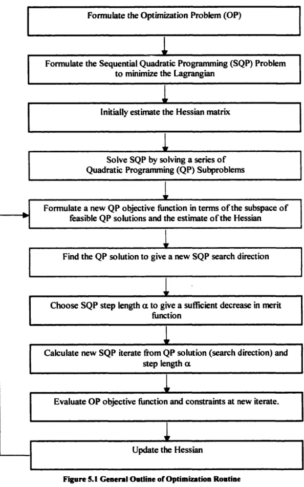
5.1 The Optimization R outine...68
5.2 Problem Statem ent... 73
6. Static Bridge/Static T ru ck ... 77
6.1 Static Bridge/Static Truck Problem ... 77
6.2 Uniform Sampling M ethod... 80
6.4 Random Sampling M ethod...90
6.5 Chapter Conclusions and Contributions... 100
7. Dynamic Bridge/Static T ru ck ... 102
7.1 Dynamic Bridge/Static Truck-Speed and Axle Spacing K n o w n ... 102
7.2 Dynamic Bridge/Static Truck-Speed and Axle Spacing U nknow n... 107
7.3 Chapter Conclusions...117
8. Static Bridge/Dynamic T ru ck ... 119
8.1 The Measured P rofile...119
8.2 Approximating the F o rc e ... 120
8.3 Parameter Identification-Optimization Routine...125
8.4 Parameter Identification-Force Objective Function...126
8.5 Parameter Identification-Deflection Objective Function... 133
8.6 Chapter Conclusions...143
9. Dynamic Bridge/Dynamic T ru ck ... 146
9.1 Simulating the Truck and Bridge-Full M odel... 147
9.2 Approximate Force M o d el... 148
9.3 WIM Algorithm... 152
9.4 Parameter Identification...152
9.5 Optimization R esults...154
9.6 Numerical R esults...177
9.7 Conclusions and Contributions...197
10. Conclusions and Future W o rk ... 200
10.2 Future Woric...204 11. References... 206
List of Figures
Figure 1.1 Flowchart o f WIM System s...5
Figure 1.2 Force Identification M ethods... 10
Figure 2.1 Flowchart o f Bridge Models in the Literature...17
Figure 2.2 Finite Element Model o f B ridge... 23
Figure 2.3Sample Deflection Profile o f the Static Bridge Midpoint D eflection...25
Figure 2.4 Sample Deflection Profile o f the Midpoint Deflection Using the Dynamic Beam M odel...29
Figure 2.5 Error Using Modes 1,2, 3, 5, 7 in the Reduced Order M odel... 33
Figure 2.6 Error Using Modes 1,2, 3 ,4 , 5, 6, 7 in the Reduced Order M odel... 33
Figure 2.7 Deflection at Each Node Due to a Moving Point F orce...35
Figure 2.8 Sine Term at Each Node For Three M odes...36
Figure 3.1 Flowchart o f Truck Models in the Literature... 42
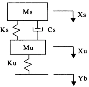
Figure 3.2 'Quarter-Car' Model Used in This W o rk ...48
Figure 4.1 Flowchart o f Bridge/Truck Interaction Literature... 56
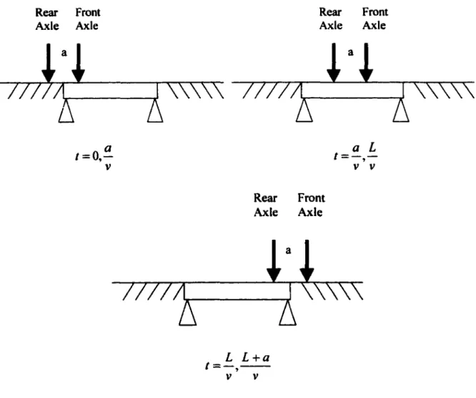
Figure 4.2 Time intervals for the Truck Crossing the B ridge... 59
Figure 5.1 General Outline o f Optimization R outine...69
Figure 6.1 Time Frames for the Truck Crossing the B ridge... 80
Figure 6.2 Midpoint Deflection Profile for the Static Bridge/Static T ru ck... 81
Figure 6.3 Changes in Force Position for Variations in Axle Spacing For a Fixed Speed at T 1 ... 83
Figure 6.4 Changes in Force Position for Variations in Axle Spacing For a Fixed Speed at T 2 ... 86
Figure 6.5 Changes in Force Position for Variations in Speed For Axle Spacing at T1 ..87
Figure 6.6 Changes in Force Position for Variations in Speed For a Fixed Axle Spacing at T 2 ...87
Figure 6.7 Front Axle Weight Estimates With Noise (Random Sam pling)... 92
Figure 6.8 Rear Axle Weight Estimates With Noise (Random Sampling M ethod) 92 Figure 6.9 Percent Error in Front Axle Weight Estimates (Random Sampling Method) .94 Figure 6.10 Percent Error in Front Axle Weight (10"^ m N o ise)... 94
Figure 6.11 Percent Error in Rear Axle W eight... 95
Figure 6.12 Percent Error in Rear Axle Weight Estimates (10^ m N o ise)... 95
Figure 6.13 Percent Error in Front Axle Weight (a)... 96
Figure 6.14 Percent Error in Front Axle Weight (b)... 96
Figure 6.15 Percent Error in Front Axle Weight (c)... 97
Figure 6.16 Percent Error in Front Axle Weight (d)... 97
Figure 6.17 Percent Error in Rear Axle Weight (a)... 98
Figure 6.18 Percent Error in Rear Axle Weight (b)... 98
Figure 6.19 Percent Error in Rear Axle Weight (c)... 99
Figure 6.20 Percent Error in Rear Axle Weight (d)... 99
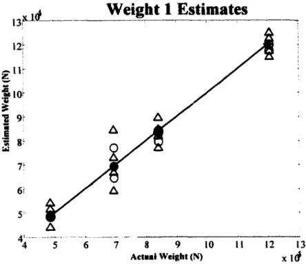
Figure 7.1 Weight 1 (Front) Estimates With Noise Using 1 M easurement...105
Figure 7.2 Weight 2 (Rear) Estimates With Noise Using 1 M easurement...106
Figure 7.3 Percent Error in Rear Axle Weight Estimates Using 1 Sensor...106
Figure 7.4 Percent Error in Front Axle Weight Estimates Using 1 Sensor...107
Figure 7.5 Static Beam Mode S hapes...108 Figure 7.6 Front Axle Weight Estimates With Noise Using 3 Sensors...I l l
Figure 7.7 Rear Axle Weight Estimates With Noise Using 3 Measurements... I l l
Figure 7.8 Percent Error in the Front Axle Weight Estimates Using 3 Measurements ..112
Figure 7.9 Percent Error in the Rear Axle Weight Estimates Using 3 Measurements ... 112
Figure 7.10 Percent Error in the Front Axle Weight Estimates (a)... 113
Figure 7.11 Percent Error in the Front Axle Weight Estimates (b)... 113
Figure 7.12 Percent Error in the Front Axle Weight Estimates (c)... 114
Figure 7.13 Percent Error in the Front Axle Weight Estimates (d)... 114
Figure 7.14 Percent Error in the Rear Axle Weight Estimates (a)... 115
Figure 7.15 Percent Error in the Rear Axle Weight Estimates (b)... 115
Figure 7.16 Percent Error in the Rear Axle Weight Estimates (c)... 116
Figure 7.17 Percent Error in the Rear Axle Weight Estimates (d)... 116
Figure 8.1 Truck Response With and Without Interaction E ffects... 122
Figure 8.2 Truck Axle F orces... 127
Figure 8.3 Front Axle Weight Estimates With Noise Using Force Objective Function .130 Figure 8.4 Rear Axle Weight Estimates With Noise Using Force Objective Function .130 Figure 8.5 Midpoint Deflection Profile for Static and Dynamic Truck M odels... 134
Figure 8.6 Front Axle Weight Estimates (Deflection Objective Function)... 136
Figure 8.7 Rear Axle Weight Estimates (Deflection Objective Fimction)...136
Figure 8.8 Percent Error in Front Axle Weight (Deflection Objective Function)... 137
Figure 8.9 Percent Error in Rear Axle Weight (Deflection Objective Function)... 137
Figure 8.10 Percent Error in Front Axle Weight (a)... 138
Figure 8.11 Percent Error in Front Axle Weight (b)... 138
Figure 8.13 Percent Error in Front Axle Weight (d)... 139
Figure 8.14 Percent Error in Rear Axle Weight (a)... 140
Figure 8.15 Percent Error in Rear Axle Weight (b)... 140
Figure 8.16 Percent Error in Rear Axle Weight (c)... 141
Figure 8.17 Percent Error in Rear Axle Weight (d)... 141
Figure 9.1 Dynamic Bridge/Dynamic Truck and Static Bridge/Static Truck Deflection Profiles... 148
Figure 9.2 Dynamic Bridge/Dynamic Truck and Static Bridge/Static Truck Deflection Profiles... 149
Figure 9.3 Front Axle Weight Estimates With N o ise ... 154
Figure 9.4 Rear Axle Weight Estimates With N o ise ... 155
Figure 9.5 Percent Error in Front Axle Weight ( a ) ... 156
Figure 9.6 Percent Error in Front Axle Weight ( b ) ... 156
Figure 9.7 Percent Error in Front Axle Weight ( c ) ... 157
Figure 9.8 Percent Error in Front Axle Weight ( d ) ... 157
Figure 9.9 Percent Error in Rear Axle Weight ( a ) ... 158
Figure 9.10 Percent Error in Rear Axle Weight ( b ) ... 158
Figure 9.11 Percent Error in Rear Axle Weight ( c ) ... 159
Figure 9.12 Percent Error in Rear Axle Weight ( d ) ... 159
Figure 9.13 Front Axle, Low Mode, Frequency Estimate (a)... 160
Figure 9.14 Front Axle, Low Mode, Frequency Estimate (b)... 161
Figure 9.15 Front Axle, Low Mode, Frequency Estimate (c)... 161
Figure 9.17 Front Axle, Low Mode, Damping Estimate (a)... 162
Figure 9.18 Front Axle, Low Mode, Damping Estimate (b)... 163
Figure 9.19 Front Axle, Low Mode, Damping Estimate (c)... 163
Figure 9.20 Front Axle, Low Mode, Damping Estimate (d)... 164
Figure 9.21 Front Axle, High Mode, Frequency Estimate (a)... 164
Figure 9.22 Front Axle, High Mode, Frequency Estimate (b)... 165
Figure 9.23 Front Axle, High Mode, Frequency Estimate (c)... 165
Figure 9.24 Front Axle, High Mode, Frequency Estimate (d)... 166
Figure 9.25 Front Axle, High Mode, Damping Estimate (a)... 166
Figure 9.26 Front Axle, High Mode, Damping Estimate (b)... 167
Figure 9.27 Front Axle, High Mode, Damping Estimate (c)... 167
Figure 9.28 Front Axle, High Mode, Damping Estimate (d)... 168
Figure 9.29 Rear Axle, Low Mode, Frequency Estimate (a)... 168
Figure 9.30 Rear Axle, Low Mode, Frequency Estimate (b)... 169
Figure 9.31 Rear Axle, Low Mode, Frequency Estimate (c)... 169
Figure 9.32 Rear Axle, Low Mode, Frequency Estimate (d)... 170
Figure 9.33 Rear Axle, Low Mode, Damping Estimate (a)...170
Figure 9.34 Rear Axle, Low Mode, Damping Estimate (b)... 171
Figure 9.35 Rear Axle, Low Mode, Damping Estimate (c)... 171
Figure 9.36 Rear Axle, Low Mode, Damping Estimate (d)... 172
Figure 9.37 Rear Axle, High Mode, Frequency Estimate (a)... 172
Figure 9.38 Rear Axle, High Mode, Frequency Estimate (b)... 173
Figure 9.40 Rear Axle, High Mode, Frequency Estimate (d)... 174
Figure 9.41 Rear Axle, Low Mode, Damping Estimate (a)... 174
Figure 9.42 Rear Axle, Low Mode, Damping Estimate (b)... 175
Figure 9.43 Rear Axle, Low Mode, Damping Estimate (c)... 175
List of Tables
Table 2.1 Properties Used in Beam M odel... 24
Table 2.2 Sine Term for Each M ode...37
Table 3.1 Numerical Static Truck Param eters... 53
Table 3.2 Numerical Parameters for Dynamic Truck Models... 54
Table 6.1 Upper and Lower Bounds for Optimization Parameters...79
Table 6.2 Average Error in Truck Parameters Using the Random Sampling Method . ..93
Table 6.3 Maximum Error in Truck Parameters Using the Random Sampling Method . 93 Table 7.1 Upper and Lower Bounds for Optimization Parameters... 104
Table 7.2 Average Errors in Axle Weight Estimates With N o ise-...107
Table 7.3 Upper and Lower Bounds for Optimization Parameters-... 109
Table 7.4 Average Axle Weight Error for the Multiple Sensor-... 110
Table 7.5 Maximum Axle Weight Error for the Multiple Sensor... 110
Table 8.1 Upper and Lower Bounds for Optimization Parameters... 126
Table 8.2 Average Error in Axle Weight Estimates Using the Force Objective Function ... 129
Table 8.3 Front Axle Frequency Estimates (Force Objective Function)...131
Table 8.4 Front Axle Damping Ratio Estimates (Force Objective Function)... 132
Table 8.5 Rear Axle Frequency Estimates (Force Objective Function)...132
Table 8.6 Rear Axle Damping Ratio Estimates (Force Objective Function)... 133
Table 8.7 Average Percent Error in Axle Weight (Deflection Objective Function) 135 Table 8.8 Maximum Percent Error in Axle Weight (Deflection Objective Function) ...135
Table 8.10 Front Axle Damping Ratio Estimates (Deflection Objective Function) 142
Table 8.11 Rear Axle Frequency Estimates (Deflection Objective Function)... 143
Table 8.12 Rear Axle Damping Ratio Estimates (Deflection Objective Function)... 143
Table 9.1 Average Error in Axle Weights Using Unlimited Optimization Iterations ....154
Table 9.2 Truck I Estim ates... 177
Table 9.3 Truck 2 Estim ates... 178
Table 9.4 Truck 3 Estim ates... 179
Table 9.5 Truck 4 Estim ates... 180
Table 9.6 Truck 5 Estimates... 181
Table 9.7 Truck 6 E stim ates... 182
Table 9.8 Truck 7 Estim ates... 183
Table 9.9 Truck 8 Estim ates... 184
Table 9.10 Truck 9 Estim ates... 185
Table 9.11 Truck 10 Estim ates...186
Table 9.12 Truck 11 Estim ates... 187
Table 9.13 Truck 12 Estim ates...188
Table 9.14 Truck 13 Estim ates...189
Table 9.15 Truck 14 Estim ates...190
Table 9.16 Truck 15 Estimates...191
Table 9.17 Truck 16 Estim ates...192
Table 9.18 Truck 17 Estim ates...193
Table 9.19 Truck 18 Estim ates...194
Acknowledgements
I would like to thank my committee as well as my professor Dr. Harold Stalford for their assistance in completing this work. I would also like to thank Sandia National Laboratories for giving me the opportunity to complete my work there, as well as Kent Pfeiffer, my mentor at Sandia, for his support and assistance over the last year.
I would also like to thank my parents for their backing and encouragement while completing this work. Without their help (with everything from school to the laundry!), I could have never gotten through all o f the ups and downs of college and graduate school. And, last but not least, I would like to thank my friend Angela for not only giving me a place to crash while finishing this work, but also for making sure that I had a lot o f fun along the way.
Abstract
In this work, we discuss the development o f a bridge weigh-in-motion (WIM) algorithm to predict axle weights to witliin 1% for ±lxlO'^m measurement noise. WIM systems that use bridges as scales are already in limited use, but they are only able to predict axle weights to within 10-15%, in part due to the models used to represent the bridge and the truck. We are proposing a method to estimate truck axle weights, axle spacing, and speed that includes the dynamic properties o f both the bridge and the truck, as well as the static effects o f the truck weight, therefore, improving the axle weight estimates. Estimates o f the truck’s dynamic properties, including natural frequencies, damping ratios, and initial conditions, are also found.
To identify the truck, the deflection profiles over time at given measurement locations are calculated. An optimization routine is then employed to determine the set of truck parameters that produces the closest match to the “measured” deflection profile. Throughout this work, the bridge is modeled as a simply-supported Euler beam. Two truck models are used to represent the truck. The first treats each axle o f the truck as a moving point force and considers only the static weight of each axle. Using this static truck model, only axle weights and axle spacing are unknown and treated as optimization parameters. The second truck model is a 2 degree-of-freedom ‘quarter-car’ model that represents the static weight as well as the dynamic behavior o f the truck. The coupled bridge/truck equations o f motion are developed and integrated to expressly include the interaction between the two. In this model, the static axle weights and axle spacing are again unknown as are the natural frequencies, damping ratios, and initial conditions o f
each mode o f each axle. Both truck models assume that the truck travels at a constant speed, and that the truck’s total time on the bridge is known from another source.
The final algorithm is developed in stages using increasing levels o f complexity in the models. In the first case, the static bridge model, which neglects the inertial properties of the bridge, is used in conjunction with the moving point force model. In the second, the dynamic properties o f the bridge are included, and the moving point force model is again used to excite the bridge. In the third and fourth cases, the dynamic, ‘quarter-car’ model o f the truck is used to excite the static and dynamic bridge respectively.
To identify the relevant properties of the dynamic truck, an approximate model of the force applied by each axle is assumed. The force is assumed to be the superposition o f the static weight o f each axle and a homogeneous solution o f the ‘quarter-car’ equations of motion. This homogeneous solution consists of two damped oscillatory modes, in which the natural frequencies, damping ratios, and initial conditions are unknown and are used as optimization parameters along with the static weight and axle spacing.
In the dynamic bridge/dynamic truck system, it is necessary to integrate the differential equations o f motion o f the coupled bridge/truck system. To do this, it is necessary to transform the truck system of equations in terms o f the unknown parameters in the homogeneous solution. This transformation is the first major contribution of this dissertation. The transformation allows the original system o f equations, which is expressed in terms o f the physical parameters stiffness, damping, and mass, to be written in terms o f the modal parameters o f the truck. Expressing the truck system in this manner eliminates the need for additional optimization parameters but still allows the integration o f the coupled bridge/truck equations inside the optimization routine.
It is necessary to integrate the bridge/truck equations o f motion at each iteration o f the optimization routine. It was found that approximately 7,000 iterations were necessary to identify the truck. Each integration takes approximately 5 seconds, resulting in approximately 10-12 hours o f computation time for each truck. This lengthy time scale prevents real-time identification o f each truck.
The second major contribution o f this dissertation is the ability to determine static axle weights very accurately, as well as the dynamic properties o f each axle. Other authors have considered identifying the static weight or the total applied force o f the truck but expressly identifying the natural frequencies, damping ratios and initial conditions o f each axle is unique to this method. Since the dynamic properties o f the truck are included in the approximate force model, they are therefore determined by the optimization routine. This algorithm determines not only the static axle weight and axle spacing o f the truck, but also provides very accurate estimates o f the natural frequencies and damping ratios of each axle. The estimation o f the dynamic properties o f each axle is unique to this algorithm and provides useful information about the passing truck.
Using this algorithm, axle weights could be determined to within 0.019% for zero measurement noise. The natural frequency and damping ratio o f each axle’s low mode could be determined to within 0.5 Hz and 0.8% (of critical damping) respectively. The properties o f each axle’s high mode could be determined to within 1.3 Hz and 3.1% (of critical damping). Measurement noise was also added to the deflection profiles to determine its effect on the algorithm’s performance. With the addition o f measurement noise o f ± lx lO'^m, estimates o f axle weights remained within 0.03%. The frequency and damping o f the low mode could be found within 0.85 Hz and 2.1% (of critical damping)
and the high mode could be identified to within 1.9 Hz and 3.4% (of critical damping). The largest measurement noise examined was ±lxlO"*m. With this level o f noise, the error in axle weight estimates remained below 1.15%. The natural frequency and damping o f the low mode could be determined within 2 Hz and 3.6%, and the high mode was determined to within 4.4 Hz and 14% (of critical damping).
Chapter 1
WIM Systems and Force Identification
Methods
A great deal o f work has been done over the years on modeling, simulating, and identifying the characteristics and behavior o f highway bridges and vehicles, both independently o f one another and o f the coupled systems. This work has been especially useful in aiding in bridge design and maintenance, as well as for developing regulations for truck loads and traffic control.
In recent times, there has been a great deal o f attention paid to the condition o f the nation’s roads and bridges. In 1989, the Federal Highway Administration gave a substandard rating to 41% o f the bridges in the U.S. highway system (“Exclusive, 1989). The poor condition o f the nation’s roads and bridges is, in part, due to the increased munber and weight o f the heavy truck traffic traveling these highways (Cebon, 1999). In 1987, it was estimated that the repair and replacement o f the faulty bridges would require a $2.65 billion investment annually for the next 20 years (“Fragile”, 1988). The potential for this exorbitant expense has prompted even more work to be done to effectively model bridges and trucks, as well as their interaction with one another.
Vehicle-induced bridge vibration is a significant contribution to the degradation o f the surface and structure o f highway bridges. While not typically the cause o f catastrophic bridge failure, it does contribute to surface wear and concrete cracking.
which can lead to corrosion (Cebon, 1999). Understanding and potentially reducing this vibration could lead to the extension o f the services lives o f many bridges and roadways, resulting in significant monetary savings for the responsible agencies.
Improving the condition o f bridges and extending their service lives is two-fold. It would be possible to better design bridges to be less susceptible to truck-induced vibration or to reduce the effects o f vibration through some sort o f structural control. Better regulation and design o f truck suspensions and loads would also be beneficial to the condition o f both the bridges and roadways. One way to accomplish the latter would be to better enforce truck weight regulations on the nation’s highways. This is the focus o f this work-to develop a system to determine truck weights as they traverse a highway bridge based on the vibration of that bridge.
The standard method of weighing trucks and enforcing weight regulations is through the use of stationary weigh stations. These stations require trucks to exit the highway and be weighed while at rest on scales. The weigh stations are manned at all times while operational. While the use o f static scales is the simplest and most obvious method o f monitoring truck loads on the highway, it is not always the most effective. Besides being costly to staff and maintain, they are easily and often avoided by drivers o f overweight vehicles since their location can be known miles in advance through driver communication (Snyder, 1992). For these reasons, there has been a great deal o f work to develop weigh-in-motion (WIM) systems to reduce the dependency on static weigh stations.
There are currently several types o f WIM systems in limited use around the world. The majority o f them fall into three main categories-systems mounted on the road
surface, systems installed in the roadbed, and systems that use bridges as scales. While there are advantages and disadvantages to all types o f systems, their use is becoming more desirable and commonplace as the need to monitor traffic grows. Many patents have been issued for different types o f systems, and a study on the effectiveness o f WIM systems was performed by the Transportation Research Board in 1986 (Transportation Research Board, 1986). Descriptions o f a few o f the primary systems are given in the following section.
A chart outlining several individual WIM systems is given below in Figure 1.1. The systems described are representative o f the types o f systems currently in commercial production and use around the world.
1.1 In-Service WIM Systems
One common type o f WIM system essentially consists o f scales embedded in the surface o f the road aligned with the wheel paths o f oncoming vehicles. The standard design o f these systems is a steel frame housing various numbers o f load cells or other electromechanical devices to measure the force from a passing vehicle. A piece o f the road surface is removed and the system is placed level with the road surface. Typically, two o f these frames are installed in each lane to align with the wheel paths o f oncoming vehicles. Patents for the systems developed by Yamanaka (Yamanaka, 1974) and Tamamura (Tamamura, 1977) issued to the same company (Yamato Scale Company, Limited) outline two systems o f this type. In Yamanaka’s system, one platform is embedded in the pavement in the path o f the vehicle. The signal recorded at the front and rear edges o f the platform are averaged to yield the weight o f the vehicle. Tamamura’s
system is similar, but it averages the response from several smaller platforms placed in a series along the wheel path. The systems proposed by Mills (Mills, 1990) and Loshbough (Loshbough, 1991) are similar to the others, although the construction details o f the frame and platform over which the truck passes vary slightly. All o f the systems average a very few measurements o f the force applied by the truck over time and/or space to yield the total weight and axle weights o f the vehicle.
I
I
On a bridge
(> 10%)
On a bridge (<l%)
(open problem)
In the Roadbed
On the road surface
Leming Mills (1990) Yamanaka (1974) Loshbough (1991) Tamamura (1977) Ibanez (1985) Muhs (1993) Golden River Corp. (1986) Snyder (1985,1992)
A study performed by the Transportation Research Board (Transportation Research Board, 1986) examined operational and installation problems and performance o f a number o f commercially produced systems similar to the ones described above. Although the companies’ products described above were not specifically discussed, systems with similar installation and operation were evaluated. It was found that such systems were quite useful in obtaining truck information in multi-lane, high traffic environments, because each lane could accommodate an individual system, making simultaneous, uncoupled measurements possible. Initial installation o f the systems was cited as a problem since traffic had to be diverted and large pieces o f the roadway surface removed to house the WIM apparatus. It was also found that, since these systems are placed in a hole in the roadway surface material, it was possible for them to work loose over time as the surrounding surface material degraded. This problem was solved by constructing another slab in the bottom o f the hole to which the frame was bolted, making installation even more time consuming and expensive. The problem o f scale avoidance was also not solved by such a system. Once the systems were identified by drivers, changing lanes or straddling lanes if the systems were installed in multiple lanes provided unusable information. Some systems were modified to correct for this problem by creating a continuous platform that spanned all lanes. While this method prevented avoiding the scale, it did not allow for independent measurements o f side-by-side vehicles. Despite many o f the problems, at the time o f publication o f the Transportation Research Board’s report, this type o f WIM system was the most widely used.
Another type o f WIM system that is growing in popularity is placed temporarily on the road surface. Typically the housings o f these systems consist o f a rubber or
elastomeric pad that is fixed to the roadway surface in the wheel path o f the vehicles. Different types o f electric or optical sensors are imbedded in these pads to measure the force imparted by a truck. Steel sheets separated by layers o f rubber are used as parallel- plate capacitive sensors in the Golden River Corporation Design (Transportation Research Board, 1986). As the rubber is compressed, the change in capacitance is measured and correlated to a truck weight. Ibanez (Ibanez, 1985) and Muhs (Muhs, 1993) use a similar rubber pad, but embed optical fibers and attenuating devices that, when compressed by a passing vehicle, attenuate the light passed through the fibers. The measured light intensity is then correlated to a weight. Other systems use inductive loops rather than capacitors or optical fibers to detect the force.
These very portable, surface-mounted systems are growing in popularity around the U.S. They have been found to be quite reliable since there are few moving parts and they are simple to install, reducing the potential for human error. They are also much less expensive than the embedded systems discussed previously, and installation is simpler, much faster (an hour as opposed to multiple days), and, consequently, much less expensive. It has been found that these types o f systems are more susceptible to intentional damage by drivers than the below-the-surface models since heavy braking can quickly deteriorate the rubber pads in which the sensors are installed. It was also found that it was necessary to install such systems on very smooth sections of roadway as surface irregularities caused a serious degradation in performance (Transportation Research Board, 1986).
The bridge WIM in motion system developed by Snyder (Snyder, 1985, 1992, Transportation Research Board, 1986) is one o f the few o f its kind in use in the U.S. It
consists o f a system o f strain gages installed on the girders underneath a bridge deck to record the bridge’s response to a passing vehicle over time. Each bridge is individually calibrated using a slowly moving test truck to determine its response to the moving load. Axle sensors at the entrance and exit o f the bridge are installed to determine the number and spacing o f the axles as well as the vehicle speed. Details o f the authors’ algorithm to determine axle weight will be discussed in the following section.
Although Snyder’s system is one o f few bridge WIM systems in use in the U S, it was found to perform very well by the Transportation Research Board. Once a bridge was instrumented, the strain gages and associated electronics remained functional for long periods of time and did not require recalibration often, fhe axle sensors at the entrance and exit o f the bridge were cited as the primary problem with the hardware o f the system, since they required stopping traffic to install, were easily damaged by vehicles, and were difficult to install in damp or below freezing conditions. Errors in the system’s weight estimates cited by the inventor (Snyder, 1985) were on the order o f 10- 15%. It is the opinion o f this author that this level o f error is due in part to the algorithm used to deduce weight from the measured strain record, as will be discussed in a subsequent section.
Although several construction, installation, and operational variations exist in commercial WIM devices, the above outlines the primary structure o f existing systems. Due to the need for more effective traffic monitoring, WIM is becoming an attractive alternative and addition to stationary weigh stations, prompting extensive and on-going work in the area. In the following section, algorithms associated with moving force identification will be addressed.
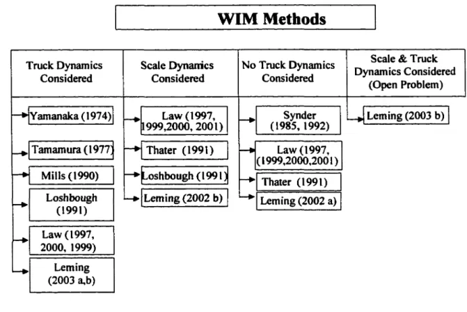
1.2 WIM Methods
The primary goal o f any WIM system is to accurately estimate axle weights and/or gross weights o f vehicles in motion. Therefore, while the structure o f the system is important, designing the hardware is not the only aspect to WIM. Developing an algorithm that accurately predicts these weights is also a necessary part o f solving the WIM problem. Several authors, as well as the inventors o f the systems described in the previous section, have worked to develop methods to determine truck characteristics from WIM data. A chart o f some o f the contributions in this area is given below in Figure 1.2. The methods used in many o f the in-service systems described above as well as work
Scale & Truck Dynamics Considered (Open Problem) No Truck Dynamics Considered Truck Dynamics Considered Scale Dynamics Considered Law (1997, (1999,2000,2001) |Loshbough(1991) Thater (1991) Leming (2002 a) Yamanaka (1974) Mills (1990) Leming (2002 b) Leming (2003 b) Tamamura (1977 Thater (1991) Synder (1985, 1992) Law (1997, 1999,2000, 2001) Loshbough (1991) Law (1997, 2000, 1999) Leming (2003 a,b)
W IM Methods
Figure 1.2 Force Identification Methods
To develop an algorithm to accurately predict truck characteristics from data acquired while the vehicle is in motion, it is necessary to first understand precisely what is being measured. As a vehicle moves along a real roadway or bridge, it does not apply a constant force over time. Irregularities in the road surface or interaction with a bridge or platform over which it travels can potentially excite the dynamics o f the vehicle’s suspension and tires, resulting in a time-varying force to be applied by the vehicle. Further details o f this tire force will be discussed in a later chapter, but to examine the problem o f moving force identification in regards to a truck, it is important to recognize that what is being measured is not necessarily a constant force.
Varying levels o f complexity in the models and algorithms used to predict static weight &om time-varying data exist in the literature and the in-service systems. Some
inventors, such as Ibanez and Muhs (Ibanez, 1985, Muhs, 1993) do not consider the dynamic nature o f the vehicle or the weighing device over which it travels, but rather make measurements over a short period o f time and ignore the time-varying aspect o f the tire force. Other inventors use a method o f averaging a very few measurements made of each axle over time to account for the time varying nature o f the tire force. The systems developed by Yamanaka (Yamanaka, 1974) and Mills (Mills, 1990) make two measurements at the leading and trailing edges o f the plate as an axle passes over and averages them to obtain an estimate o f the static weight. In a similar method, Tamamura (Tamamura, 1977) averages the force measurements obtained from a series o f 2-4 successive platforms to estimate the weight.
It could also be said that the dynamic properties o f the scale, whether it be a platform embedded in the pavement or a bridge structure, such as in Snyder’s work (Snyder, 1985, 1992), must be considered to obtain accurate measurements o f the tire force. Loshbough’s system (Loshbough, 1991) handles the problem o f scale platform dynamics by designing the platform to have a natural frequency far from that o f the truck’s so that the two do not interact and successive measurements o f tire force do not contain the effects o f the vibrating scale platform.
The system designed by Snyder (Snyder, 1985, 1992) uses a bridge structure as a scale platform. This means that the weighing platform is much larger and more flexible than the other systems discussed, and the vehicle remains on the platform for a much longer period o f time. Measurements o f the strain in the bridge girders are made continuously over time, so there are many measurements to work with. Each bridge is characterized by an influence line (the bending moment at a given measurement location
versus force position along the bridge for a unit load). This influence line can be approximated by the influence line o f a beam with equivalent geometry and bending properties as the sum o f the girders or by direct measurement. To obtain the influence line directly, a slowly moving truck passes over the bridge, and measurements are made at each o f the sensor locations. The truck travels across the bridge slowly enough that neither the bridge dynamics nor the truck dynamics are excited. The magnitude o f the line is then normalized by the weight o f the truck.
Axle sensors at the entrance and exit o f the bridge record the number and spacing o f the axles, and the speed is also calculated using this information. Assuming a constant speed, the position o f each axle is therefore known at every point in time. A system o f equations is generated at each time step that relates the measured strain to the product o f the appropriate value along the influence line for each axle and the unknown axle weights. To solve this system o f equations, it is necessary that there be at least as many measurement locations as axles o f the truck. The equations are then solved for the unknown axle weights at each time step. To account for the dynamic nature o f both the bridge and the truck, the axle weights obtained at each time step are then averaged to give an approximate static weight. The estimates o f axle weight reported by the author (Snyder, 1985) show errors up to 15%. Although Snyder does not speculate on the origin o f this error, recent studies in the literature indicate that this is approximately equal to the error found in simulating a bridge’s response to a dynamic truck crossing a bridge when the interaction between the truck and the bridge is neglected, as it is in Snyder’s model, (Green and Cebon, 1997).
Other authors in the literature are also working on the identification o f moving forces from bridge response information. Some o f the work involves attempting to eliminate the dynamic properties o f the measured signal to extract the only the static response. Thater et al. (Thater, et al., 1991) developed a method to filter the dynamic bridge response using the pre-determined response o f the bridge to a slowly moving vehicle (“static” response). They had previously determined that using conventional filtering methods were not effective for separating the dynamic and static responses o f the bridge. Working in the frequency domain, it was assumed that the static and dynamic responses o f the bridge at 0 Hz to the same truck were equal. An FFT was performed on both the static bridge response due to the calibration test truck and the measured dynamic response o f an unknown truck. The magnitude o f the dynamic response at 0 Hz was then scaled by the magnitude o f the static response to the calibration truck at 0 Hz to determine the unknown weight. While this method provided some improvement in weight estimates over the existing bridge WIM techniques, errors o f 5% using simulated data were still observed.
Another group. Law, et al. (Law, 1997, 1999, 2000, 2001) is also working on the moving force identification problem, although their goal is not to extract the static weight o f a simulated truck crossing a bridge, but rather to identify numerically the total force applied by the truck. Modeling the bridge as a simply supported Euler beam, two types o f moving forces are examined. First, a static point force moving at a constant speed along the beam is used to excite the bridge. Next, a simple vehicle model that includes interaction with the bridge due to the displacement o f the bridge under each contact point is used. Details o f this vehicle model wUl be discussed in a later chapter.
For both the moving point force and the vehicle model, the differential equation o f motion for the deflection o f an Euler beam (neglecting damping) is developed. For the point force analysis, a closed form solution is obtained for the deflection o f the beam as a function o f space and time, and expressions for the bending moment and acceleration are derived from this. Either the moment or acceleration at a given sensor location is used as the measured bridge response, and the number o f measurement locations is greater than or equal to the number o f point forces moving across the beam. A system o f equations for each point in time is then formulated based on the measured bridge response and the closed form solution with the magnitudes of the point forces assumed to be unknown. Solving these equations leads to an estimate of the magnitude o f each point force for each instant in time. In the point force case, these estimates are averaged to determine the magnitudes o f all point forces.
To determine the magnitude o f the moving vehicle model’s force, coupled differential equations o f the vehicle and the bridge are formulated. This formulation will be discussed in greater detail in a later chapter along with the model. To first obtain the “measured” (obtained through simulation) bridge response to the vehicle model, the coupled, nonlinear equations are numerically integrated to obtain deflection, moment, and acceleration profiles at the sensor locations over time. Using the same method as above, a system o f equations is formed for each time step using either bending moment or acceleration as the measured quantity. The equations are then solved for the magnitude o f the applied force at each time step. This method was not intended to determine axle weights, but rather to identify the magnitude o f the applied force at each instant. Random white noise o f various magnitudes was also added to the measured signal to determine the
performance. Using this method, errors in force magnitude estimates o f both the point force and the vehicle model ranged from 6-24% for the smallest noise level.
The goal o f our work is to develop an algorithm that relates a measured bridge response to a set o f truck parameters including axle weights, axle spacing and speed that produced the bridge response. In certain cases, speed is assumed to be known from an independent sensor. Different models o f both the truck and the bridge are examined which include both moving point forces and moving vehicle models. The effect o f the bridge dynamics on our ability to determine truck properties is also examined by first neglecting and then including the inertia o f the bridge. A simply supported Euler beam model is used to represent the dominant behavior o f the bridge, and both point force and one-dimensional axle models described in later chapters are used to simulate a truck. An optimization routine minimizes the least-squares difference between the measured profiles and the simulated ones and modifies relevant truck parameters to obtain the best approximation o f the truck characteristics. The different models and combinations o f models used as well as the optimization technique will be outlined throughout the remainder o f this work.
Chapter 2
Bridge Models
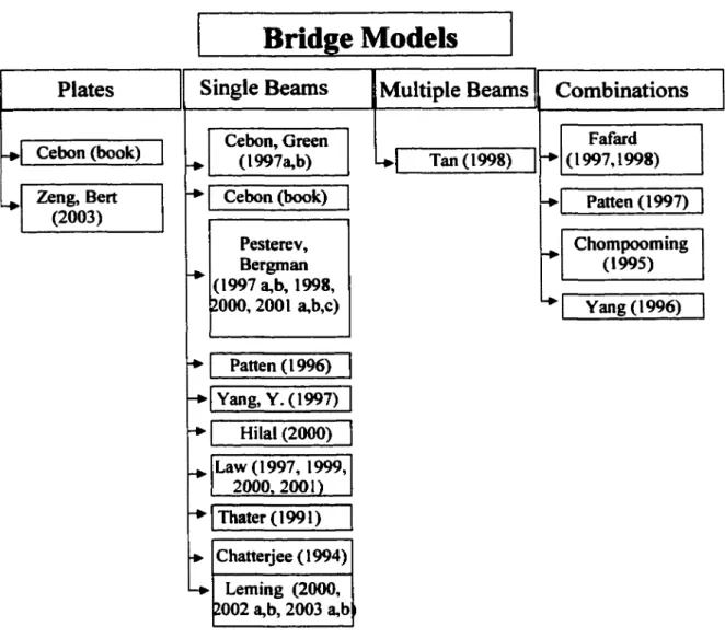
Examining the response o f bridges to different loadings is a large area o f research, focusing on a variety o f different driving forces. Response to wind, earthquake and vehicle loading comprise a significant portion o f the work in structural dynamics. A portion o f this work deals with modeling bridges to obtain their response to excitation by vehicles. Many authors are also working in this area and using a variety o f different types o f models. These models vary in structure as well as in level o f complexity. A chart outlining some o f the contributions in the area o f bridge model construction and solution is given below in Figure 2.1. The works have been categorized by the geometric properties o f the model.
Bridge Models
Plates Single Beams [ M ultiple Beams Combinations
Cebon(book) Cebon, Green (I997a,b) T an(1998) (1997,1998)Fafard Zeng, Bert
(2003)
Cebon (book) Patten (1997) Pesterev, Bergman (1997 a,b, 1998, 2000, 2001 a,b,c) Chompooming (1995) Yang (1996) Patten (1996) Yang, Y. (1997) Hilal (2000) Law (1997, 1999, 2000.2001) Thater (1991) Chatteqee (1994) Leming (2000, 2002 a,b, 2003 a,b
Figure 2.1 Flowchart o f Bridge Models in the Literature
2.1 Combination Models
Different authors use varying degrees o f complexity to model bridges, depending on their purpose. Some o f the most complex models are finite element representations o f a given bridge that include a variety o f elements, including plates, beam, solids, shells and bars. One such model developed by Patten and Sun (Sun, 1997) included the bridge’s superstructure and piers for use in the design o f a vibration mitigation system. It was a 4,800 degree o f freedom (DGF) model composed o f three types o f beam elements, thin shell, bar, and solid elements, and 811 nodes. The accuracy o f the model was
verified experimentally, and it was found that the first eight natural fiequencies matched those o f the actual bridge upon which the model was based to within 3%. Higher modes, up to the 14***, were also predicted with slightly less accuracy. To use this model more efficiently, a coarser meshing technique was used which resulted in only 225 DOF but maintained the accuracy in predicting the first ten modes o f the bridge (Patten, 1999).
The model was based on an in-service interstate highway bridge on 1-35 N near Purcell, Oklahoma. Since this bridge is the basis for other models used in the body o f this text, some important conclusions drawn from Patten’s work should be discussed here, although geometric and construction details will be given in the following section. First, the first two modes o f the bridge were found to be bending modes o f frequencies 2.5 and 3.0 Hz. Higher modes were torsion and combinations of torsion and bending (Sun, 1997). It was also found that standard trucks crossing this bridge excited only those modes below 10 Hz (the first fourteen modes for the actual bridge). An even simpler model o f this bridge was also used in much o f the practical application o f this group’s work. It was found that modeling this bridge as a simply supported beam with the appropriate mass, stiffriess, and damping properties gave sufficient performance and computational efQciency to design the authors’ vibration control system. Time domain measurements compared favorably with those from the actual bridge and the full-scale finite element model (FEM), making it attractive for estimating deflection. It is on this simplified beam model that the bridge models used in the following chapters are based.
Other authors have also constructed finite element models that are combinations o f a variety o f elements. One common method for doing this is to model the bridge deck using plate/shell elements and to model the girders independently using beam elements.
Fafard (Fafard et al., 1998, Fafard and Bermur, 1997) and Chompooming (Chompooming and Yener, 1995) both constructed this type o f model. Fafard’s model also included the parapet and a sidewalk on one side o f the bridge and modeled them using beam elements. The model also used a non-uniform set o f bending properties to more fully capture the cracks and irregularities in the concrete deck. This model was quite accurate in predicting the modal characteristics o f the first ten modes, but showed large variations o f up to 70% in the prediction o f strain along the bridge for various vehicle induced loadings. The authors attribute a significant portion o f this error to the fact that the surface roughness of the actual bridge is not included in the model, which would change the response o f the simulated vehicle model. Variations in the actual vehicle dynamics and the simulated one were also cited as a source o f error in these calculations. Chompooming’s model was very similar in structure to Fafard’s although it included only the deck and the girders and not the parapet or any other parts o f the bridge structure. The majority o f their work dealt with the influence o f vehicle parameters, which will be discussed in the following chapters.
Many o f these combination-type models most accurately predict the finer points o f the bridge response, including many modes and a variety o f mode shapes, but they can also be computationally intensive and time consuming to use. Simplified models that include important features o f the bridge response are often developed to predict specific aspects o f interest to the author. In Cebon’s book (Cebon, 1999), two simplified models were developed and compared to experiment and to each other. The first model was a mesh o f orthotropic plate elements mounted on flexible supports. To incorporate the effect o f the girders, the plate elements were given different stifftiesses along the
direction o f the girders than in the other direction. In the second model, the beam was approximated as a simply-supported beam with mass and stifhiess properties representative o f the deck and girder cross sections. The responses o f both models were then compared to measured data from the actual bridge. It was found that the beam model predicted only four o f the first eight modes while the plate model was relatively accurate for them all. However, in examining time domain data, it was found that both the plate and the beam model gave accurate and nearly identical deflection information when compared to the measured response to various loads. This was attributed to the fact that the two dominant modes o f this particular bridge were bending modes and were represented well by both models. The author concludes that either model would suffice for accurately obtaining deflection information for this bridge, but computation time and complexity would infiuence the choice o f model.
2.2 Multiple Beam Models
Other models of highway bridges that use only beams have also been examined. These models typically represent the bridge as either a single beam along the direction o f the bridge or as a grillage or mesh o f beams to include both transverse deflections and torsional effects. One such grillage model o f a bridge was constructed by Tan (Tan, et al. 1998). The model used beam longitudinal beam elements to represent the girders and transverse diaphragms to represent the torsional stiffness. The two types o f elements were pinned at their intersection to ensure equal deflections at these nodes. The stiffiiess and geometric spacings were tuned so that the static deflections measured fi-om an actual
bridge corresponded to ones simulated using the model, but does not compare the dynamic response o f the two.
2.3 Single Beam Models
One o f the simplest types o f models used to simulate a bridge’s response is a single or multi-span beam. As discussed previously, this type o f model captures the dominant behavior o f many types o f bridges (Cebon, 1999, Patten, et al. 1999), although it does not include the torsional effects o f the bridge deck. In terms o f computational efficiency, however, beam models are usually considered much more practical for actual use. Extensive work has been done using beam models to examine not only bridge response, but also interaction effects between vehicles and bridges. Different methods o f solving the coupled systems have also been proposed. Pesterev and Bergman (Pesterev and Tavrizov, 1994 a,b, Pesterev and Bergman, 1997 a,b, 1998, 2000, Pesterev et al, 2001 a,b) did extensive work developing efficient and accurate methods to solve the bridge-truck interaction problem using a beam model. Their emphasis, however, was on the solution rather than the model, and details o f their work will be discussed in the next chapter.
Many other authors also use beam models to study the interaction between vehicles and bridges. Yang (Yang, Y. 1995, 1997) used such a model to study the interaction between railway bridges and trains. They used regular beam elements o f appropriate cross-section and properties where the train was not in contact and proposed an “interaction” element where the train was in contact. This element included the mass, stiffiiess, and damping o f the combined beam/vehicle system. Hilal (Hilal and Zibdeh,
2000) used beam models with a variety o f boundary conditions to examine the effects o f acceleration, deceleration, and uniform motion o f a moving point force and obtained a closed form solution for the deflection profile. Chatteqee (Chatteqee et al., 1994) used a multi-span beam model that allowed torsion o f the beam due to eccentric loads. The bridge on which this model was based had much higher frequencies in torsion than in bending, meaning that it was torsionally stiff. This resulted in a negligible change in bridge deflection when torsional coupling was included, indicating that, for this bridge, the eccentricity o f the vehicle with respect to the center-line o f the beam had did not have an effect on bridge behavior. Results were not given for a less torsionally stiff bridge.
Because o f the computational efficiency, beam models were chosen to use in the rest o f this work. Single span, simply supported beams are used to determine the bridge response to a variety o f load conditions. We also examine the effect o f the inertia o f the beam on the response o f the bridge to a loading and on our ability to identify that load. Details o f these models are given in the following sections.
2.4 My Models
The goal o f this work was to identify the axle weights, axle spacing, and speed o f a truck passing over a bridge based on the deflection response of the bridge. To do this, it was necessary to develop a model o f the bridge that would be representative o f the principal behavior o f the bridge when subjected to vehicular loading. An in-service highway bridge spanning Walnut Creek on 1-35 N near Purcell, Oklahoma was the basis for the simplified beam models used in this work. The original bridge consisted o f a reinforced concrete deck and five steel I-beam girders spanning the entire length o f the bridge. The four-span bridge was supported by three equally spaced piers and two end
abutments. The right-hand traffic lane was centered over the second girder (near east) and the left-hand lane was centered between the fourth and fifth girders (near and far west) (Sun et al., 1997). For simplicity, a single span beam model based on the above described bridge was developed for this work. It is important to note that this model and the force identification method could easily be extended to include more lanes.
The general model consisted o f eight beam elements and nine nodes. It was found that this number o f elements was sufficiently large to accurately represent the displacement while still remaining computationally efficient. The use o f eight elements was also advantageous, because it provided nodes at locations that were desirable for measurements, the midpoint, the quarter-length point, and the three-quarter-length point. A diagram o f this model is given below with the potential sensor locations marked in Figure 2.2. A discussion o f these sensor locations will fjc given below in section 2.4.
E,I,p,A
Midpoint % Point
V* Point
Figure 2.2 Finite Element Model o f Bridge
Each node was given two degrees o f freedom (DOF), vertical displacement and in-plane rotation. The boimdary conditions o f the simply supported beam were such that the displacements at the first and last nodes were fixed. In total, this model had 16 DOF. The properties o f the beam were determined to correlate with the measured properties of the second span o f the Walnut Creek Bridge. These properties are given below in Table 2.2.1.
Table 2.2.1 Properties Used in Beam Model
L 30.48 m
El (product) 7.36x10'® Nm^
pA 3.35x10" kg/m
Two versions o f this beam model were used in this work. The first, termed the “static” model, did not include the inertia o f the beam, the solution o f which was a series o f static calculations through time. The second, the “dynamic” beam, included the inertia o f the beam and was solved continuously.
2.5 Static Beam
Three methods o f solving the static beam response were used, the finite element method, the direct solution of the differential equation o f motion o f the beam for a moving point force, and static beam bending equations. Details o f the solution for a moving vehicle model will be given in the Interaction chapter o f this work.
2.6 Finite Element Model
The first solution method used the finite element model and properties given above. The elemental stiffness matrix Kg was derived using the standard beam element equations and is given below in Equation (2.1). The global stiffiiess matrix was assembled using standard finite element method and will not be given here for the sake o f brevity. 12 6Z 6L AÛ - 1 2 - 6 L 6L 2Û - 1 2 6L - 6 1 21? 12 - 6 1 - 6 L AI? (2.1)
For the moving point force problem, a static calculation o f the beam deflection was performed at each time step to determine the displacement o f each node. Although the same beam model was used for a moving vehicle model, a slightly different solution method was employed and will be discussed in Chapter 4. In both cases, however, the governing equation o f the bridge deflection was given by
f ( r ) = K c x ( ( ) (2.2)
the solution o f which is given by
x ( ,) = K g - 'F ( ,) (2.3)
where Kc is the global stifhiess matrix o f the beam, x(t) is the deflection and rotation at each node, and F(t) is a vector o f the applied force at each node.
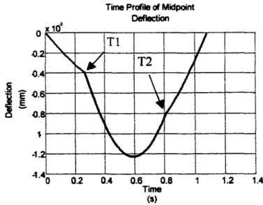
The term deflection profile’ will be used throughout this work to define the deflection as a function o f time at a given sensor location. An example of a profile using the static bridge finite element model is given below.
-0.: -0.4 - 10.0â 0 . 8 --1 r -1.2 --1.
Time Profile o f Midpoint
$ 0 2 0.4 0.6 0.8 1 1.2 1.4
Time
Figure 2.3Sample Deflection Profile o f the Static Bridge Midpoint Deflection
The measurement equation, giving the beam deflection at the sensor location is given by
ÿ = C g x “ [^3x3 2]
C B (1,8) = l for midpoint deflection (2.4)
C B (2,4) = 1 for quarter point deflection Cb(3,12) = 1 for three-quarter point deflection
for three sensor locations. For only one sensor located at the span midpoint, Cb is a 1x32
vector and Cb( 1,8)=1.
2.7 Solution of the Differential Equation
The second method for determining the deflection profile o f a static beam subjected to a moving force involves the solution o f the partial differential equation o f bending for a beam. This method o f solution assumed a moving point force, although it was expanded for use with a moving vehicle model. For this section, however, we will limit our discussion to moving point forces only.
The differential equation o f bending for a Bemoulli-Euler beam is given by
(2.5)
where w(x,t) is the vertical displacement o f the beam as a function o f time and horizontal distance along the length, x, P is the force, and x(/) is the location o f the force as a function o f time. A solution to this equation in terms o f the mode shapes o f the beam can be written as
w(x,r)=2^^.(x)F;.(/) (2.6)
/=i
For a simply supported beam, the mode shapes,^(5r), can be written as
Substituting Equations (2.6) and (2.7) into Equation (2.5) and multiplying both sides by sin ^ ^ ^ leads to
sin— s i n " ^ ^ . ( / ) = P ^ ( j c - x ( r ) ) s i n ^ (2.8)
If Equation (2.8) is integrated with respect to x from 0 to L, the right-hand side becomes zero except where x = x(f). The equation then becomes
The left-hand side o f Equation (2.9) is zero unless i=j, when it is undefined. Applying L’Hospital’s rule with respect to the quantity i-J, the left-hand side becomes
(2.10)
The above equation gives an expression for the time-dependent portion o f the solution to Equation (2.4). The complete solution to Equation (2.5) is therefore given by
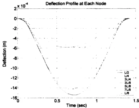
Evaluating Equation (2.11) at the sensor locations generated deflection profiles o f the same nature as in Figure 2.3. It was determined that using 4-5 terms o f the series expansion in Equation (2.11) gave the best approximation to the finite element deflection profiles. Equation (2.11) was evaluated at x=L/2, L/4, 3L/4 to measure the deflection profile.
The standard equations for static beam bending were also used to evaluate the deflection profiles o f the beam. The deflections due to each force at a given location are found using the standard expressions for the inverse o f beam stiffiiess and are given below (Gere, 1997). Ht is used if the x<b, and H2 is used if x>b, where x is the location
o f the applied force along the beam.
H (v- j ) - ~ ~
6EIL
(2.12)
where and ai+bi=L. The deflection o f the beam is given below in three different time frames which determine how many axles on the beam at a given time. The details o f the truck motion will be given in Chapter 3. Wi and fP? are the front and rear axle weights o f the truck, a is the spacing between the weights, and v is the truck speed. The subscripts / and j depend on the relative location o f the sensors and each applied force.
w{x,t)=-H.(x,b^ j(x,b^)W^ w { x ,t) = - H f^ x ,b ^ ^ when 0 < / < — V when — < t< — . L ^ ^ L - ¥ a when — < / < ---V V (2.13)
The sensors are located at the midpoint and/or the quarter-point and three-quarter- point (x=L/2, L/4, 3L/4). The deflections at these locations would be given by evaluating Equation (2.13) at these points.
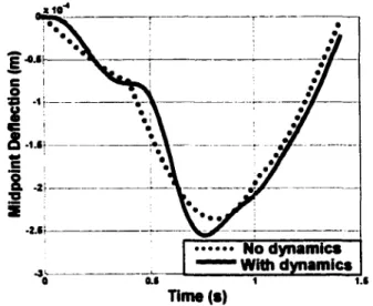
2.9 Dynamic Beam
The second version o f the beam model used in this work included the inertial effects o f the bridge and was termed the “dynamic” bridge model. The same eight
element, nine node geometric model o f the simply supported beam was used, but the mass of the beam was included in the development. The figure below illustrates a deflection profile o f the midpoint deflection o f the beam using this model compared with one firom the static model.
«10'
-2.t{
No dynamics With dynamics Time(s)
Figure 2.4 Sample Deflectlou Profile o f the Midpoint Deflection Using the Dynamic Beam Model
A consistent mass matrix for a beam element was developed using the parameters given in Table 2.2.1, and is given below in Equation (2.14). The same element stiffiiess matrix was used as in the static model. Equation (2.1). The global mass and stiffiiess matrices were assembled using the standard finite element method.
M pAL 420 156 22L 54 -1 3 L 22Z 4£? 131 -3 1 ? 54 131 156 - 2 2 L - \3 L -3Û - - 2 2 1 4Û-(2.14)
The damping in bridges is typically quite low (approximately 2% o f critical) (Cebon, book). The measured values o f the damping in the Walnut Creek Bridge are
quite close to 2% for the first eight modes o f the actual bridge. Using the 2% damping, the global damping matrix is therefore given by
Cc =0.04Mc(Mg- 'Kc)^ (2.15)
where Ma and Kc are the global mass and stiffiiess matrices respectively. The discretized equations o f motion for the beam becomes
M^xCr) + K j { t ) = F i t ) (2.16)
where x(t) is again the displacement and rotation o f the nodes, and F(t) is a vector of force applied at each node.
To conveniently integrate these equations, it is necessary to reduce the set of second order differential equations to a set o f first order ones
(2.17)
where Xg =[x x f and Ab and Bs(t) are given below ./(t) is the time force vector. This quantity will be discussed for individual truck models in later chapters. Cg varies depending on which o f the three potential sensor locations are being measured.
A g — 016x16- I
I
16x16 -1, BB 016x16 - 1 R(s,z) (2.18) Cg —[0 3^3 2] Cg(l,8) = l Cg(2,4) = l Cg(3,I2) = Ifor midpoint deflection for quarter point deflection for three - quarter point deflection
A " i t ' ^ ■
node i £ i node i+l
where R(s,z) describes the distribution o f the force and moment due to the load between the modes as described below.
2.10 R(s^)
For a force applied at a position z, 0<z<[., 0 < s ^ /8
For zeEj, and 0 < s ^ /8 , the 32x1 vector (or 32x2 for two axles) R(s^> is formed from an 36x1 (or 36x2) vector r(s^ ) whose elements are defined below. Each column o f R (s^) represents the location o f an individual axle.
r(5,z)2,_, = j^ { 2 s ^ - 3 s - L + û ) ris,z)„ = j ^ ( s ^ L - 2 s - Û + s ü )
ris, z)2t,2 = ^ ( - 2s^ + 3 f" A ) (2 .2 0 )
ris,z)2„.2 = - ^ { s ^ L - s ^ l} )
All other r(s,z)j = 0 for 2i -2 > j > 2i + 2
The boundary conditions are such that the deflections at the endpoints o f the span are zero. For this reason the 1®*, 17*, 19*, and 35* rows o f r(s«z) are removed (r(s,z)i=[ ], r(s,z)i7=[ ], etc.) to form R (s^).