Counting Human Flow with Deep Neural Network
Shing H. DoongShuTe University [email protected]
Abstract
Human flow counting has many applications in space management. This study applied channel state information (CSI) available in IEEE 802.11n networks to characterize the flow count. Raw inputs including mean, standard deviation and five-number summary were extracted from windowed CSI data. Due to the large number of raw inputs, stacked denoising autoencoders were used to extract hierarchical features from raw inputs and a final layer of softmax regression was used to model the flow counting problem. It is found that this deep neural network structure beats other popular classification algorithms including random forest, logistic regression, support vector machine and multilayer perceptron in predicting the flow count with attractive speed performance.
1. Introduction
Human flow counting has many applications in space management. For example, the flow count can be used to prevent over-crowdedness or to adjust HVAC settings accordingly. Mechanical units are commonly used to count human flow. However, they are inefficient and inconvenient. Image based solutions have been developed, but they require expensive camera devices and illumination and occlusion problems are unavoidable in image processing.
The average human being contains about 60~70% water which disrupts radio wave propagation. Research on intelligent space management has shifted from image based solutions to methods based on wireless technologies that are widely deployed in today’s smart societies. Wireless based solutions avoid the privacy invasion issue that often comes with image based approaches.
Lin et al. exploited radio irregularity in the Internet of Things to count people automatically [1]. The researchers used features extracted from received signal strength indicator (RSSI) to count the flow. RSSI, an aggregate power indicator resulting from the
multipath propagation of indoor wireless communication [2], is widely available in many devices. RSSI is coarse-grained and more detailed communication information called channel state information (CSI) has been defined in the IEEE 802.11n standard.
Using hardware fast Fourier transform, off-the-shelf network interface cards such as Intel WifiLink 5300 (IWL) can output channel frequency response (CFR) as 30 CSI data per communication channel [3]. CFR is to RSSI what a rainbow is to a sunbeam [2].
CSI has a finer resolution than RSSI regarding communication channels, and exhibits a more stable temporal feature as well. Using empirical data, Wang et al. showed that CSI amplitude had a greater stability than RSSI for continuously received packets at a fixed location [4]. The finer resolution comes with the price of higher dimensionality of CSI based features. Deep learning techniques were used in [4] to properly reduce the dimension and improve indoor localization accuracy.
Deep learning, a rejuvenated artificial neural network research subject, has caught the attention of many researchers in artificial intelligence. An essential part of deep learning is deep neural networks (DNNs) that automatically capture useful features from raw inputs for classification problems [5][6][7][8]. For example, with the high dimensional CSI data, a well designed DNN may be able to extract features that are helpful to the flow counting task.
In this study, we exploited the opportunity of rich CSI data embedded in 802.11n networks to count human flow automatically. The counting problem was defined as a classification problem, i.e., using patterns of CSI fluctuation to predict the corresponding flow size. With 3 receiving antennas and 1 transmitting antenna (i.e., 3 communication channels), each packet creates 90 CSI amplitude data. Over a window of n continuously received packets, these 90n data were summarized into 630 raw inputs for the flow counting problem. Principal component analysis (PCA) is often used to extract or select features from high dimensional inputs before a classification algorithm is applied to the training data [9]. Instead of PCA, we applied stacked
Proceedings of the 51st Hawaii International Conference on System Sciences|2018
URI: http://hdl.handle.net/10125/49987 ISBN: 978-0-9981331-1-9
denoising autoencoders (SdA) [10] to extract hierarchical features from our raw inputs. On top of the SdA, a softmax regression was used to classify the last encoded features into different flow sizes.
Our data set has a size of 16000 records. Though the volume by no means fits the definition of big data, the large number of raw inputs may create a complicated situation for traditional classification algorithms. Our goals of this study include (1) to empirically validate the acclaimed advantage of pre-training in DNN [11]; and (2) to compare the efficacy of DNN with that of other classification algorithms including multilayer perceptron, multinomial logistic regression [12], random forest [13] and support vector machine [14] in the human flow counting problem.
This paper is organized as follows. Section 2 is devoted to a literature review on CSI, autoencoders, DNN and various other classification algorithms. Methodology and experimental data sets are described in section 3 followed by experimental results and discussions in section 4. We conclude the paper with remarks in section 5.
2. Literature review
Automatic flow counting has been investigated by many research groups. Device-free approaches are preferred because they do not require people to carry specific devices such as RFID to do the job. Recent research tends to exploit radio irregularity patterns caused by human movement to predict the flow size. We first describe CSI data revealed by 802.11n networks, which are very popular in today's public or private space. Autoencoders are unsupervised neural networks that can be trained easily. We explain the goal and training of autoencoders next. When layers of autoencoders are stacked and a classification network such as the softmax regression is placed on top of the SdA, we obtain a DNN in deep learning. We explain the pre-training and fine-training stages of a DNN and regularization techniques used to prevent overfitting a DNN. Finally, we briefly discuss other classification algorithms used in this study to compare their efficacy with that of DNN.
2.1. Channel state information
Let h(t) denote a temporal linear filter, known as channel impulse response (CIR), that models the multipath propagation of a wireless communication channel. A channel is defined as a pair of a transmitting antenna and a receiving antenna. If s(t) is the transmitted signal, then the received signal r(t) =
s(t)⨂h(t) is the convolution of s(t) and h(t). Taking
the Fourier transform of both sides, we obtain R(f) =
S(f)H(f) where H(f), called CFR, is the Fourier
transform of h(t). It is known that environmental changes cause CIR to fluctuate only in a few time indices; on the other hand, diverse frequency spans make CFR a more responsive descriptor for such changes [2]. By modifying IWL's network driver, Halperin et al. [3] release 802.11n CSI tool that can output sampled values of CFR as CSI.
A subcarrier is a communication sub-band in the orthogonal frequency division multiplexing (OFDM) modulation scheme used by 802.11n networks. For a 20 MHz communication channel, OFDM divides the channel into 64 subcarriers each with 312.5 KHz space. Of these 64 subcarriers, 802.11n uses 52 subcarriers for data, 4 for pilot and 8 as null. IWL network driver further aggregates the 56 data and pilot subcarriers into 30 groups of which the modified driver in [3] reports the sampled CFR values as CSI. Thus, CSI of each communication channel contains data from 30 subcarriers.
Because IWL is a popular network card and CSI provides fine-grained channel information, recent exploitations of radio signals in indoor applications have been mostly based on CSI instead of RSSI. For example, CSI was used in [4] to infer indoor localization. Zhang et al. used CSI to identify an individual because different people have different walk gaits [15].
2.2. Autoencoders
Autoencoders are unsupervised networks used to extract internal patterns from data. A typical autoencoder has 3 layers: the input layer, the hidden layer and the output layer (Figure 1). The hidden layer serves the purposes of encoding inputs into more compact representations that may embed certain patterns of data. The output layer decodes codes in the hidden layer. The purpose of training an autoencoder is to obtain network weights so that outputs match inputs as closely as possible.
The decoding weights do not have to be related to encoding weights. In figure 1, we use tied weights to reduce the number of weights, i.e., the decoding matrix is the transpose of the encoding matrix. At the hidden layer and the output layer, each node gets its value from the activation of a weighted sum of inputs from the previous layer. We used the sigmoid function
1/(1 + e−s) as the activation function in this study.
The hidden layer does not have to be of a smaller size than the input layer. In order to avoid the learning of a trivial identity function, regularizing functions can be added to a loss function to guide the search of optimal weights. In this study, we used an L2
regularizer of network weights and mean squared errors to construct the loss function (equation 1). In equation 1, xi's are inputs from a data set, zi's are
corresponding outputs from the network with weight matrix W, and C is a tradeoff parameter that balances the effect of mean squared errors and network weights, i.e. ‖W‖2= �∑ wij ij2. Gradient decent based methods are used to adjust W iteratively so that loss(W) is as small as possible.
loss(W) =1n∑ ‖xni=1 i− zi‖2+ C‖W‖2 (1)
Vincent et al. considered denoising autoencoders to extract robust features from the original data [10]. To train a denoising autoencoder, inputs are first corrupted to simulate noise that may be embedded in the original data. Then corrupted inputs move forward the network to produce outputs as usual, and loss is obtained by comparing uncorrupted inputs with outputs from the corrupted inputs. Using a binomial distribution, we randomly set an input node to zero to produce a corrupted input.
Figure 1. An autoencoder network
2.3. Deep neural networks
After a denoising autoencoder is trained, we can remove its decoding layer and use its encoding layer to extract new features from the original inputs. Using outputs from the encoding layer as new inputs, we can train the next layer of denoising autoencoder. This procedure can be continued successively for a few layers of denoising autoencoders extracting hierarchical features from the original inputs. Eventually, we put a supervised layer on top of the last encoding layer. A typical supervised layer is the softmax layer where each output node represents the probability for the occurrence of a class.
When the loss function in equation 1 is measured by cross entropy instead of mean squared errors, the
softmax layer is equivalent to multinomial logistic regression in statistics [12]. Due to a neat expression, most software packages implementing multinomial logistic regression can optimize the loss function by using Newton's or quasi-Newton's algorithms. Newton's algorithms not only consider second derivatives of the loss function, but also invert a Hessian matrix. In short, Newton's algorithms take more efforts to conduct an epoch of training, but may also need fewer epochs to find the optimal solution. In the following, we will call multinomial logistic regression with Newton's or quasi-Newton's optimization the Logistic classifier. We reserve the term Softmax classifier for a softmax layer trained with gradient decent based methods.
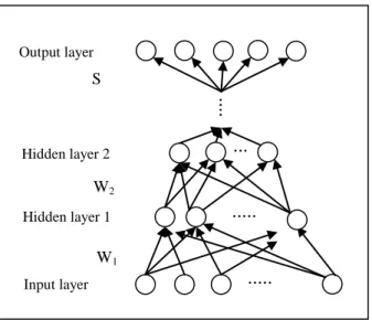
A typical DNN is shown in Figure 2, where the hidden layers (W1, W2, ...) are encoding layers of
successively trained denoising autoencoders, and the output layer (S) is a softmax layer. The pretraining stage of a DNN refers to the greedy layer-wise training step of SdA without the softmax layer, i.e. each denoising autoencoder is trained individually. The first denoising autoencoder is trained with the original inputs, the second autoencoder is trained with the encoded data from the first autoencoder, and so on. The fine-training stage of a DNN is to train the entire network as a whole, but layers of SdA are initialized with the weights from individually trained autoencoders. Erhan et al. showed that the unsupervised pretraining step helped a DNN to generalize better on test data [11].
A multilayer perceptron (MLP) in this study has the same network structure as a DNN except that its hidden layers are not pretrained with SdA. That is, during training, MLP initializes its weights with randomly selected numbers. MLP is a powerful learning tool when many hidden layers are used. Training MLP with random initial weights may lead to two problems: optimization and generalization. The optimization issue refers to the problem that solutions may be trapped in unwanted local optimal areas, and the generalization issue refers to the problem that the trained MLP does not perform well on test data [11].
...
...
...
Input layer Hidden layer Output layer W WTFigure 2. A deep neural network
2.4. Other classification algorithms
Multinomial logistic regression is a simple two layer structure where the activation function is the softmax function in equation 2. Since each node represents the probability of an output class, cross entropy (negative log-likelihood) is commonly used for the loss function. A weight regularizing term may be added to the loss function as in equation 1. Newton's algorithms are available to minimize the loss function.
σ(𝐳𝐳)𝑗𝑗 = 𝑒𝑒
𝑧𝑧𝑗𝑗
∑𝐾𝐾𝑘𝑘=1𝑒𝑒𝑧𝑧𝑘𝑘, 𝑗𝑗 = 1,2, … , 𝐾𝐾 (2)
As a powerful ensemble algorithm, random forest (RF) creates multiple decision trees in the training stage and aggregates decisions from these trees to make predictions in the operational stage [13]. Each decision tree is trained with data sampled with replacements from the training set. At a decision node, RF picks the best variable from a random subset of predictors by using entropy or Gini criterion. Using multiple decision trees in the operational stage may prevent the overfitting problem encountered in many machine learning algorithms.
Support vector machine (SVM) is a popular classification algorithm based on statistical learning theory. SVM uses a kernel trick to map inputs into a high dimensional feature space where data of different classes may be more easily separated. Commonly used kernels include radial basis kernels (equations 3) and polynomial kernels (equation 4). A separating hyperplane with the maximum margin is sought in the feature space. With kernel tricks, distances in the feature space may be easily computed by using the kernel function and the margin maximization problem
in the feature space is converted to a convex quadratic programming problem in the input space. SVM is best suited for binary classification problems where the maximum margin separating hyperplane can separate two classes in the feature space. When SVM is applied to multiclass classification problems, multiple one-over-rest or one-over-one binary classifiers are trained to predict outputs of multiple classes.
K(𝐱𝐱, 𝐳𝐳) = exp(−γ‖𝐱𝐱 − 𝐳𝐳‖2) (3)
K(𝐱𝐱, 𝐳𝐳) = (𝐱𝐱 ∙ 𝐳𝐳 + c)d (4)
3. Methodology
We describe our experimental scenario to collect CSI data. Raw inputs are summarized from a window of CSI data. These inputs are processed with a DNN to construct a human flow counting system. Network structure of the DNN is explained next.
3.1. Experimental scenario
In an experimental scenario, groups of one to five people were asked to walk through a corridor where two Linux systems were placed by the sides (Figure 3).
Figure 3. Experimental scenario
Systems T and R were Ubuntu systems installed with the modified IWL network driver from [3]. They were placed 6 meters apart and 75 centimeters above the floor. The groups were asked to walk in a row at about the same pace to pass the line of sight (LoS) between T and R. System T continuously transmitted packets with one antenna at the speed of 1000 packets per second. At the same time, system R received these packets with three antennas and recorded their CSI data for later processing. Thus, there were 3 communication channels in this scenario. For each group size (one to five), 20 walk-throughs were
T R Human flow LoS
...
...
...
W1 W2....
S Input layer Hidden layer 1 Hidden layer 1 Hidden layer 2 Output layerconducted, and each walk-through lasted about 8 seconds.
3.2. Input extraction
For each walk-through, we divided the collected data into 160 non-overlapping windows. Each window consisted of CSI data from 50 packets (50 milliseconds), and was summarized as follows.
Let zi,j,kdenote the CSI absolute value for the ith
receiving antenna, the jth subcarrier and the kth packet, where i = 1, 2, 3, j = 1, ..., 30 and k = 1, ..., 50. Then we used mean, standard deviation and five-number summary to summarize CSI data of these 50 packets.
For each combination of the 3 receiving antennas and 30 subcarriers, we computed the mean, standard deviation, first quartile, second quartile (median), third quartile, minimum and maximum of zi,j,k of the 50 packets in a window. In total, there are 16000 records equally divided into five classes of flow size. Each record has 630 inputs and one output. Table 1 lists the inputs extracted from a window of 50 packets.
Table 1. Inputs extracted from
windowed CSI data (i = 1, ...,3, j=1, ...,30)
Variable Meaning
mui,j Mean of zi,j,k across 50 packets
sdi,j Standard deviation of zi,j,k across 50 packets fqi,j First quartile of zi,j,k across 50 packets sqi,j Second quartile of zi,j,k across 50 packets tqi,j Third quartile of zi,j,k across 50 packets mini,j Minimum of zi,j,k across 50 packets maxi,j Maximum of zi,j,k across 50 packets
More specifically, a record in our data set has the following format: (mu11, sd11, fq11, sq11, tq11, min11, max11 , ..., mui,j, sdi,j, fqi,j, sqi,j, tqi,j, mini,j, maxi,j, ..., mu3,30, sd3,30, fq3,30, sq3,30, tq3,30, min3,30, max3,30, class) where the first 630 components are CSI descriptive statistics as in Table 1 and the last component is a class label. In order to reduce the dimension of raw inputs, we used SdA to extract hierarchical features.
3.3. Network structures
By a rough rule of halving the inputs and a trial and error approach, we designed a DNN with three hidden layers. The first hidden layer had 300 nodes, the second had 150 nodes, and the third had 60 nodes. On top of the third hidden layer, we had a softmax layer with 5 nodes each corresponding to the probability of a specific flow count. Each hidden layer was the encoding layer of a denoising autoencoder. These
autoencoders were trained layer by layer as in most SdA studies. The pretrained weights were used as initial weights in the fine-training stage of the whole network including the softmax layer which was randomly initialized.
Table 2 shows the settings of each hidden layer. Most of these parameters were obtained via a trial and error approach or adopted from the default setting of the used DNN training package. The corruption rate (noise) was used to randomly set that fraction of input nodes equal to 0 in denoising autoencoders training. The penalizing coefficient is the tradeoff coefficient C in equation 1.
A mini-batch approach was adopted to update network weights more frequently than the traditional epoch based network training. For each autoencoder training, after a batch of 100 records had been processed, network weights were updated with Adam gradient based optimization algorithm. Each autoencoder was trained with 20 epochs. The learning rate was set to 0.001.
Table 2. Properties of hidden layers
Layer Nodes Characteristics Autoencoder training 1 300 0.1 corruption rate, 0.01 penalizing coefficient 20 epochs, batch size 100 2 150 0.1 corruption rate, 0.01 penalizing coefficient 20 epochs, batch size 100 3 60 0.2 corruption rate, 0.01 penalizing coefficient 20 epochs, batch size 100
Even with the L2 weight regularization in SdA,
DNN still overfits training data easily. Thus, dropouts were introduced to each hidden layer. In the fine-training stage, a fraction of hidden nodes were randomly marked as nonexistent (dropouts) to prevent overfitting. On the other hand, every node was used to predict the class label of a test record in the operational stage [16]. The dropout rate was 0.2 for hidden layer 1, and 0.1 for hidden layers 2 and 3.
Cross entropy was used in the fine-training stage to guide the search of optimal network weights. In addition, an L2 weight regularizer was added to the loss
function with a penalizing coefficient of 0.01. Adam optimization algorithm was adopted for 300 epochs of network training with a batch size of 200.
The above network structure with pretraining will be denoted as DNN in the following report. Another neural network with the same structure without pretraining will be denoted as MLP. MLP used random numbers to initialize weights of hidden layers.
The third network will be denoted as Softmax in the following report. Softmax has two layers: the input layer of 630 nodes and the output layer of 5 nodes. The softmax function (equation 2) was the activation function of this network. In contrast to Newton's algorithm in multinomial logistic regression (Logistic), Softmax was trained with Adam gradient based optimization algorithm. The batch size and the number of epochs were the same as those of DNN and MLP.
All three neural networks were modeled and trained with the open source Tensorflow package from Google [17]. To minimize the programming efforts, we used the Keras framework [18] on top of Tensorflow. Inputs were normalized column-wise so that each predictor had a maximum value of 1.
3.4. Settings of the other classifiers
RF and Logistic classifiers were implemented with the Weka software [19]. The RF algorithm was set to use a forest of 300 decision trees and the number of randomly selected predictors at a decision node was set to 10. Regarding the logistic regression in Weka, we selected a ridge coefficient of 0 and a maximum iteration number of 300 to train the model. Weka used a quasi-Newton's method to minimize the loss function.
Since Weka had no built-in support for SVM, we turned to the scikit-learn python library [20] for SVM classifiers. Unlike other classifiers in this study, SVM is inherently a binary classification algorithm, and scikit-learn uses the one-over-one approach to handle multiclass classification problems. The following default settings were used with scikit-learn: radial basis kernels (equation 3) with regularizing coefficient C=1 and automatic setting of γ.
4. Experimental results and discussions
In this study, we have implemented 6 models to count human flows with the help of machine learning: DNN, MLP, Softmax, RF, Logistic and SVM. Before comparing their efficacy, we first describe how data analysis was conducted.4.1. Data analysis procedure
Cross validation (CV) is a powerful tool to assess classification accuracy in machine learning. For a k-fold CV, a data set at hand is first partitioned into k equal parts randomly. One part of the partition is reserved as the test set while the remaining parts are combined to form the training set. After a classification assessment is done with these training and test sets, the next part of the partition is reserved as the test set
while the remaining parts are combined to form the training set, and another classification assessment is conducted. This process of training and test continues until each part of the partition takes the role of test set exactly once. Then prediction rates from k assessments can be averaged to get a final result for this CV.
Obviously, the final result of a CV depends on its partition of the data set. Thus several runs of k-fold CV should be conducted to minimize the effect of data partitioning. Our data set has 16000 records, each with 630 predictors and one class label. We used 5-fold CV to evaluate the performance of the six models stated above. In addition, 20 runs of 5-fold CV were conducted with each run using a specific seed to initiate the partitioning step. In a training and test step of the 5-fold CV, there were 12800 training records and 3200 test records. Using random permutation, we ensured that each output class (1 to 5) was equally represented in the training set and the test set.
4.2. Result from RSSI based inputs
In order to appreciate the advantages provided by fine-grained CSI data in flow counting, we conducted a rough prediction analysis by using inputs from RSSI. As the modified driver in [3] also reports the RSSI value of each communication channel, we gathered 3 such values from our experimental setup. Like the CSI case, a window of 50 packets was used to summarize RSSI values in a very short period. The windowed RSSI values were summarized by the mean, standard deviation and five-number summary. Instead of 630 predictors, we had 21 predictors from RSSI values of 3 communication channels. A typical run of 5-fold CV with different algorithms (MLP, Softmax, RF, Logistic, SVM) yielded a prediction rate from 0.470 to 0.520. This result is much worse than the following result from CSI based inputs.
Though the above result seems very unattractive, we need to note that this is a 5-class prediction problem. Since each class is equally represented in test sets, a naive guess with one consistent class label yields a prediction rate of 0.2. Procedures with random guesses may yield even lower prediction rates.
4.3. Result from CSI based inputs
Table 3 summarizes prediction rates of the six models with CSI based inputs in Table 1. The mean column is the average rate from 20 runs of 5-fold CV. The Stand. Dev column represents the standard deviation of these 20 prediction rates, and the Run Time column indicates the number of seconds used to run a training and test step of a CV. All analyses were
done on a machine equipped with Intel i7-6700 CPU, 16GB of DDR4 memory and NVIDIA GTX 1050 GPU with 4GB of video ram.
Table 3. Prediction accuracy
Mean Stand. Dev Run Time
DNN 0.827 0.0027 56 s MLP 0.817 0.0032 46 s Softmax 0.709 0.0016 50 s RF 0.739 0.0016 41 s Logistic 0.746 0.0019 93 s SVM 0.780 0.0014 324 s
The run time column shows that SVM had the longest run time to conduct a training and test step of a 5-fold CV. This could be due to the fact that a large number of one-over-one binary classifiers needed to be trained. For a 5-class classification problem, 10 such classifiers need to be trained.
The Logistic model required the second longest run time to finish a training and test step of a CV. This can be expected because Weka implements the loss optimization procedure with a quasi-Newton's algorithm, which needs more derivative computations and inverts many large matrices.
The other models needed about the same time to finish a training and test step of a CV. The only unforeseen result was MLP ran faster than Softmax even though Softmax had a simpler network structure. This might be due to the dropout layers embedded in MLP. Dropouts reduce a network structure in the training stage.
In terms of prediction accuracy, DNN offered the highest performance among the six models considered in this study. MLP came next, followed by SVM, Logistic, RF and Softmax in turns. SVM was still a powerful classification algorithm except that it took much longer time than the other models to handle the data. The Logistic model beats its structurally equivalent Softmax model without a surprise, because Weka implements its Logistic regression with a quasi-Newton's algorithm while the Softmax model uses gradient decent based methods to optimize its loss function.
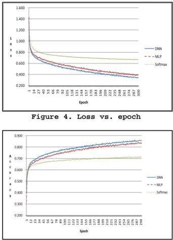
Figure 4. Loss vs. epoch
Figure 5. Accuracy vs. epoch
For the training of three gradient decent based models (DNN, MLP and Softmax), we plot the loss value and the accuracy rate epoch by epoch in Figures 4 and 5 respectively. These figures show that (1) the training procedure converged as more epochs of training were conducted; (2) the loss function based on cross entropy faithfully guided the search of optimal weights. When loss values went down, prediction rates went up; and (3) the comparison among the three models was consistent with the final result on test data.
RF was the fastest algorithm among the models considered in the study. However, its prediction accuracy was mediocre compared to the other models. On the other hand, MLP competed neck and neck with DNN in terms of accuracy and run time.
Is the 1% difference between DNN and MLP significant? Since all six models ran each of the 20 CVs with the same partition scheme, we conducted a paired t-test of prediction rates to check the statistical significance. The result shows that the 2-tail test statistic has a p-value of 3.46E-10, effectively p = 0.000 in most statistics textbooks. Thus, DNN has a significantly better performance than MLP. This result reaffirms Erhan et al.'s claim that pretraining helps a network's generalization power [11]. The 20 prediction rates from MLP seem to have a bigger standard
0.200 0.400 0.600 0.800 1.000 1.200 1.400 1.600 1 14 27 40 53 66 79 92 10 5 11 8 13 1 14 4 15 7 17 0 18 3 19 6 20 9 22 2 23 5 24 8 26 1 27 4 28 7 30 0 L o s s Epoch DNN MLP Softmax 0.200 0.300 0.400 0.500 0.600 0.700 0.800 0.900 1 1 2 2 3 3 4 4 5 5 6 6 7 7 8 8 9 1 0 0 1 1 1 1 2 2 1 3 3 1 4 4 1 5 5 1 6 6 1 7 7 1 8 8 1 9 9 2 1 0 2 2 1 2 3 2 2 4 3 2 5 4 2 6 5 2 7 6 2 8 7 2 9 8 A c c u r a c y Epoch DNN MLP Softmax
deviation (0.0032) than that of DNN (0.0027). However, the Levene's test for equality of variances does not reject the null hypothesis of equal variances (p = 0.211), thus this difference in standard deviation is not statistically significant. That is, we cannot conclude that DNN is more reliable in computing the prediction rate.
4.4. Effect of five-number summary
To investigate the effect of five-number summary on the prediction result, we conducted a second data analysis without five-number summary from CSI data. This result may reveal the impact of additional features summarized from windowed CSI data.
This time, only the mean and standard deviation were extracted from each window of 50 CSI data. The five-number summary was not included in the formation of raw inputs. Each record now has 180 predictors from the combination of 3 communication channels and 30 subcarriers.
Since the input data had a smaller dimension, we reduced the network structure accordingly. Instead of three hidden layers, we used only two hidden layers. The first hidden layer had 90 nodes and the second hidden layer had 30 nodes. A softmax layer was placed on top of the second hidden layer.
Six models were considered as before. The DNN model initialized its hidden layers with pretrained weights from SdA. Properties of the SdA are listed in Table 4. These parameters were chosen based on a trial and error approach or default values in the adopted software Keras [18]. The MLP model initialized its network weights randomly sampled from a uniform distribution.
Table 4. Properties of hidden layers
Layer Nodes Characteristics Autoencoder training 1 90 0.1 corruption rate, 0.01 penalizing coefficient 20 epochs, batch size 100 2 30 0.1 corruption rate, 0.01 penalizing coefficient 20 epochs, batch size 100
In order to prevent overfitting, dropouts were introduced for hidden layers of DNN and MLP. The dropout rate was 0.2 for hidden layer 1 and 0.1 for hidden layer 2. The supervised training of DNN, MLP and Softmax was conducted with 300 epochs and a batch size of 100. Settings for the other classifiers were the same as the previous analysis. Table 5 summarizes the prediction result of the six models.
Table 5. Prediction result
Mean Stand. Dev Run Time
DNN 0.759 0.0021 68 s MLP 0.752 0.0022 62 s Softmax 0.685 0.0012 47 s RF 0.721 0.0016 34 s Logistic 0.786 0.0013 30 s SVM 0.790 0.0011 56 s
This time, SVM was the champion in terms of prediction rate. Though 10 one-over-one binary classifiers were needed, its run time was not much different from that of the other models. This shows that when more predictors are used, it takes more time for SVM to have a convergent quadratic optimization solution.
Logistic model was the champion in terms of run time, and its predication performance was just a little bit worse than that of SVM. DNN was in the third place regarding prediction accuracy. However, its lead over MLP was still statistically significant (p = 0.000) though the absolute lead was only 0.7%.
For this second data analysis, the run time of DNN and MLP was longer than that of the corresponding network in the first analysis. This is due to the fact that we had a finer update schedule in this case (a batch size of 100 vs. a batch size of 200).
4.5. Discussions
Though both analyses reaffirm Erhan et al.'s claim that pretraining helps a network's generalization power [11], the absolute improvement of prediction rate (1% and 0.7% respectively) looks pretty small compared to results presented in most machine learning studies. In [11], Erhan et al. considered the MNIST data set which had 60000 training data and 10000 test data. Their results showed that the absolute improvement in prediction rate was less than 1% when 1 to 4 hidden layers were used. Thus, this range of improvement seems more like a norm for evaluations on data sets with 10000s of records.
By comparing Tables 3 and 5, we also observe the scalability and robustness of each prediction model in terms of the number of predictors. Though DNN and MLP failed to beat Logistic and SVM in the case of 180 predictors, they out-performed the latter in the case of 630 predictors. The results show that adding five-number summary to predictors increased prediction accuracy when right classifiers were used. Our analysis shows that Logistic and SVM did not scale well and robustly to the number of predictors. On the other hands, DNN and MLP scaled well and robustly to the
number of predictors. Part of the reason might be due to the fact that Tensorflow utilized NVIDIA GPU efficiently, while scikit-learn and Weka did not take advantages of the GPU.
In the experimental scenario, we only used one transmitting antenna to transmit packets. IWL allows the use of three transmitting antennas at the same time. With five-number summary included in the predictors, this will create a raw input of 1890 predictors. When more IWLs are placed in the field to collect CSI data, for example, two systems can be used to receive packets sent from a third system, raw inputs of more predictors will be created. From our experiments, it seems that DNN is a promising solution to handle large data sets with many predictors.
Hidden layers visualization may be useful for understanding the inner working of SdA in the field of computer vision. SdA was used to extract different levels of geometric features from the MNIST data set for the problem of digit recognition [21]. For example, the first layer may detect edges from raw input images, the second layer detects simple shapes composed of edges, and higher layers detect even more abstract geometric features suitable for automatic digit recognition. Because our raw data consist of the mean, standard deviation and five-number summary from windowed CSI data, it is probably difficult to visualize motifs discovered in different layers of SdA. This problem is similar to the construct explanation problem encountered in factor analysis.
5. Conclusions
Deep learning has revitalized artificial neural network research in machine learning. A typical DNN in deep learning has many hidden layers each pretrained with a denoising autoencoder. Literature has shown that pretraining can help DNN generalize better than an MLP without pretraining. The pretraining is efficient and effective because each autoencoder is trained individually, thus the bizarre explosion or vanishing of weights in a back-propagation training of MLP can be avoided.
We applied DNN to a human flow counting problem that may have many applications in space management. Though our data set by no means belongs to the category of big data, rich inputs extracted from IEEE 802.11n CSI data may confuse many popular classification algorithms to learn an efficient model.
Specific to the wireless based flow counting problem, we observed that CSI predictors yielded a better performance than RSSI predictors in predicting flow counts, no matter which classification algorithms were used to learn the model. This justifies the merits of fine-grained information embedded in CSI data, and
also explains recent trends of exploiting CSI data in various indoor applications.
Moving from RSSI to CSI, the number of predictors increases at least 30 times, because IWL outputs CSI data for 30 subcarriers. Each CSI entry is actually a complex number, and we only considered the modulus part (absolute value) of CSI in this study. With such fine-grained information of communication channels, high dimensional inputs provide more differentiation power for learning algorithms on the one hand, but produce the curse of dimensionality problem on the other hand. Traditional approaches to reduce input dimensions include PCA or hand-crafting domain specific features. In this study, we used SdA to automatically craft features useful for our flow counting model.
Our experiments showed that five-number summary could improve the flow counting accuracy when right algorithms were used. Overall, we found that DNN, an MLP with pretrained hidden layers, and the 630 predictors summarized from windowed CSI data in Table 1 provided the best performance.
Though DNN solves the high dimensionality problem and provides the best performance at the same time, it comes with several issues that are worthy of noting. First, many hyper-parameters need to be tuned properly in order to get a good performance, for example, the number of layers, nodes per layer, penalizing coefficients, corruption rates, epochs, batch sizes, dropout rates and so on. It seems that most studies today still rely on a trial and error approach to tune these parameters. Second, DNN inherits the black box learning characteristics of neural networks, thus it is difficult to explain the inner working of hidden layers in many application cases.
In the future, we plan to use the full capacity of IEEE 802.11n communication channels to capture CSI data. This will create raw inputs with a very high dimension. DNN will be carefully examined to investigate its learning power on such high dimensional data.
Acknowledgments. This work was supported in part by a grant from the ministry of science and technology (Taiwan) under the contract number MOST-105-2632-E-366-001. The author appreciates constructive comments from the anonymous reviewers.
6. References
[1] W. Lin, W. Seah, and W. Li, "Exploiting Radio Irregularity in the Internet of Things for Automated People Counting", IEEE International Symposium on Personal, Indoor and Mobile Radio Communications, 2011, 1015-1019.
[2] Z. Yang, Z. Zhou, and Y. Liu, "From RSSI to CSI: Indoor Localization via Channel Response", ACM Computing Surveys, 2013, 46(2), 25.
[3] D. Halperin, W. Hu, A. Sheth, and D. Wetherall, , "Tool release: gathering 802.11n traces with channel state information", ACM SIGCOMM Computer Communication Review, 2011, 41(1), 53-53.
[4] X. Wang, L. Gao, S. Mao, and S. Pandey, "CSI-based Fingerprinting for Indoor Localization: a Deep Learning Approach", IEEE Transactions on Vehicular Technology, 2017, 66(1),763-776.
[5] G. Hinton, and N. Srivastava, "Reducing the Dimensionality of Data with Neural Networks", Science, 2006, 313, 504-507.
[6] L. Deng, and D. Yu, "Deep Learning: Methods and Applications", Foundations and Trends in Signal Processing, 2014, 7(3-4), 197-387.
[7] I. Goodfellow, Y. Bengio, and A. Courville, Deep Learning, 2016, MIT Press: Cambridge, MA.
[8] Y. LeCun, Y. Bengio, and G. Hinton, "Deep Learning", Nature, 2015, 521(7553), 436-444.
[9] A. Malhi, and R. Gao, "PCA-based Feature Selection Scheme for Machine Defect Classification", IEEE Transactions on Instrumentation and Measurement, 2004, 53(6), 1517-1525.
[10] P. Vincent, H. Larochelle, Y. Bengio, and P. Manzagol, "Extracting and Composing Robust Features with Denoising Autoencoders", ACM International Conference on Machine Learning, 2008, 1096-1103.
[11] D. Erhan, Y. Bengio, A. Courville, P.-A. Manzagol, and P. Vincent, "Why Does Unsupervised Pre-training Help Deep Learning?", Journal of Machine Learning Research, 2010, 11, 625-660.
[12] S. Le Cessie, and J.C. van Houwelingen, "Ridge Estimatiors in Logistic Regression", Appl. Statist., 1992, 41(1), 191-201.
[13] L. Breiman, “Random Forests”, Machine Leaning, 2001, 45(1), pp. 5-32.
[14] C. Cortes, and V. Vapnik, "Support-vector Networks" Machine Learning, 1995, 20(3), 273-297.
[15] J. Zhang, B. Wei, W. Hum, and S. Kanhere, "WiFi-ID: Human Identification Using WiFi Signal", IEEE International Conference on Distributed Computing in Sensor Systems, 2016, 75-81.
[16] N. Srivastava, G. Hinton, A. Krizhevsky, I. Sutskever, and R. Salakhutdinov, "Dropout: A Simple Way to Prevent Neural Networks from Overfitting", Journal of Machine Learning Research, 2015, 15, 1929-1958.
[17] M. Abadi, and et al., "TensorFlow: Large-scale Machine Learning on Heterogeneous Systems", 2015, Software available from tensorflow.org.
[18] F. Chollet, "Keras", GitHub,
https://github.com/fchollet/keras
[19] E. Frank, M.A. Hall, and I.H. Witten, The WEKA Workbench. Online Appendix for "Data Mining: Practical Machine Learning Tools and Techniques", 2016, Morgan Kaufmann, Fourth Edition.
[20] F. Pedregosa, and et al., "Scikit-learn: Machine Learning in Python", Journal of Machine Learning Research, 2011, 12, 2825-2830.
[21] D. Erhan, Y. Bengio, A. Courville, and P. Vincent, "Visualizing Higher-Layer Features o a Deep Network", University of Montreal, 2009, 1341, 3.