Numerical methods for estimating linear econometric models

(1)

Numerical methods for estimating

linear econometric models

Paolo Foschi

A thesis submitted in fulfilment of the requirements for the degree of

Doctor of Philosophy

Institut d’informatique

Universit ´e de Neuch ˆatel

(2)

(3)

(4)

(5)

Abstract

The estimation of the Seemingly Unrelated Regressions (SUR) model and its variants is a core area of econometrics. The purpose of this thesis is the investigation and development of efficient numerical and computational methods for solving large scale SUR models. Specifically, its aim is twofold. Firstly to continue past successful research into the design of numerically efficient methods for estimating the basic SUR model. Secondly to extend these methods to variants and special cases of that model.

The basic computational formulae for deriving the estimators of SUR models involve Kro-necker products and direct sum of matrices that make the solution of the models computationally expensive even for modest sized models. Alternative numerical methods which substantially reduce the computational burden of the estimation procedures are proposed. Such methods successfully tackle the estimation of the basic SUR model, and that of SUR models derived from VAR(p) pro-cesses, SUR models with VAR disturbances, SUR models with unequal size observations and SUR models with orthogonal regressors. The proposed methods, are based on orthogonal transforma-tions, and thus, results to be numerically stable. Furthermore, they do not require the common assumption which is usually made in most theoretical analyses, that the disturbance covariance matrix be non-singular.

(6)

(7)

To Elisa

(8)

(9)

Acknowledgments

Firstly, I would like to thank my supervisor, Prof. Erricos J. Kontoghiorghes. He has engaged me for Ph.D. studies in Neuchˆatel which gave me the opportunity to work in the interface of Mathe-matics, Statistics, Economics and Computer Science. He gave me the flexibility to accomplish my research studies without disregarding my family needs. Further, he has always supported me and accustomed to my not always impeccable timing. Most important he has shown to be a real friend. Then my thanks, goes to Prof. Charles Broyden who, with his peculiar personality, introduced me to the beauty of numerical linear algebra and taught the importance of elegance in mathematics. I would also like to thank Prof. David A. Belsley (Boston College) who has always encouraged our research and frequently made constructive suggestions and corrections to our work.

I thank Prof. Aristide Mingozzi, Prof. Vittorio Maniezzo and Prof. Sergio Polidoro of the University of Bologna who have supported and provided me with the necessary infrastructure in Italy in order to continue my research.

I thank my friends and colleagues Cristian Gatu and Petko Yanev. Their help during my Ph.D. studies is very much appreciated. They have revealed to be splendid office mates and never refused to join me and Erricos for a coffee. I hope they will extend the research in this thesis in their specific domains.

I wish also to acknowledge the people who assisted me in accomplish the administration duties that are required by the University and State of Neuchˆatel. Specifically, I’m referring to Gianfranca Cerrito, Jaroslava Messerli, Prof. Hans-Heinrich Naegeli and Prof. Pierre-Jean Erard.

I could not avoid to acknowledge and thank the Swiss National Science Foundation which financially supported this research through the projects 21-54109.98 and 2000-061875.00.

(10)

(11)

Introduction

The estimation of Seemingly Unrelated Regressions (SUR) models have broad applicability in the analysis and estimation of econometrics models. The SUR model arise in the estimation Simul-taneous Equations (SE), Time Series and Panel Data models, to name just a few [4, 15, 58, 79]. Procedures that provide theoretically efficient estimators to SUR models with special properties and the theory of inference for SUR models have been an active research area in econometrics for more than forty years [80, 86, 89]. The computational and numerical aspects of the various proposed estimation procedures have been investigated only recently [16, 45, 46, 48, 50, 51, 53]. Eventhough, the most commonly used estimation procedures are based on the direct implementa-tion of theoretical formulae, which are computaimplementa-tionally expensive even for modest sized problems, and gives meaningless results for models with ill-conditioned matrices [6, 76]. For example, in the case of a SUR model of 10 equations with an average of 8 regressors and100 observations each, the estimation problem can be seen as equivalent to a General Linear Model (GLM) of1000

observations and80variables.

When the disturbance covariance matrix is known, the most commonly used estimator for the SUR model is the Generalized Least Squares (GLS) estimator. This estimator gives a Best Lin-ear Unbiased Estimator (BLUE). Otherwise, when the covariance matrix is unknown, the iterative Feasible GLS (FGLS) and Maximum Likelihood (ML) procedures are used. The FGLS and the ML estimators come from the solution of normal equations that involve Kronecker products, di-rect sums and with the unknown disturbance covariance matrix replaced at each iteration by an estimator until convergence has been achieved [3, 66, 69, 80, 83].

The equally important development of numerical and computational tools for solving SUR 1

(16)

models lags behind the theoretical advances made in econometrics. Algorithms for computing the BLUE of the SUR model usually require the disturbance covariance matrix to be non-singular, eventhough this is not the case in many economic applications [38, 84].

1.1 Linear Models

A common problem in statistics is that of estimating parameters of some assumed relationship be-tween one or more variables. A linear model is one relationship in which a dependent (endogenous, explained) variable y can be expressed as a linear function of independent (exogenous, explana-tory) variablesx1, . . . , xn. When there aremsamples observations this relationship can be written

as        y1 y2 .. . ym        =        x11 x12 · · · x1n x21 x22 · · · x2n .. . ... ... xm1 xm2 · · · xmn               β1 β2 .. . βG        +        ε1 ε2 .. . εm        .

whereεiis an error term for which specific values cannot be predicted. In compact form the latter

can be written as

y=Xβ+ε, (1.1)

where y, ε _∈ Rm, X _∈ Rm×n and β _∈ Rn. Additional assumptions should be specified to complete the linear model (1.1). The first assumption is that the expected value of εis zero, that is,E(ε) = 0. The second assumption is thatXis a non stochastic matrix, and thusE(XT_ε_{) = 0}_.

The final assumption is that the variance-covariance matrix ofεisσ2Ω, where Ωis a symmetric non negative definite matrix andσ is an unknown scalar. In summary the complete mathematical specification of the (general) Linear Model (GLM) is given by

y=Xβ+ε, ε_∼(0, σ2Ω), (1.2)

where the notation ε _∼ (0, σ2_Ω)_{means that the disturbance vector} _ε_{comes from a distribution}

having zero mean and variance-covariance matrixσ2Ω.

The notation used in this treatment is consistent with that used in [28, 46] and is here briefly resumed. Anm_×nmatrix with elementsai,j(i= 1, . . . , mandj= 1, . . . , n) will be denoted by

(17)

1.2. QR DECOMPOSITION AND THE ORDINARY LINEAR MODEL 3 colon-notation is used to denotes submatrices and subvectors [28]. Thekth column and row ofA are denoted by A:,k and Ak,:, respectively. The submatrix Ai:k,j:lhas dimension (k−i+ 1)× (l₋j + 1) and its first elements is given by ai,j. Similarly, vi:k is the subvector of v having (k₋i+ 1) elements and starting with vi. When the lower or upper index in the subscript is

omitted, then the default values will be one or an the upper bound of this subscript, respectively. A zero dimension denotes a null matrix or vector. For example, A_i_:_,_:_l is equivalent toA_i_:_m,_1:_l. The transpose ofAwill be denoted byAT and ifAm×m is non singular then its transpose inverse will be written asA−T_{. The}_m_×_m_{identity matrix and its}_i_{th column will be denoted by}_I

m andei,

respectively. Thus,Im= e1 e2 · · · em

. Furthermore,_·,_·Ωand

_·_F will denote the Euclidean, energy and Frobenious norms, respectively. That is,v2 ₌_vT_v_,_v2

Ω =vTΩvand

A2_F =P_im,n₌₁_,j₌₁a2_i,j, whereΩis positive definite.

1.2 QR Decomposition and the Ordinary Linear Model

The QR Decomposition (QRD) is one of the main computational tools in regression [8, 9, 11, 19, 28, 31, 57, 75]. It is mainly used in the solution of linear systems. It provides more accurate so-lutions than the LU and other similar decompositions, and involves fewer computations than the Singular Value Decomposition. The QRD is often associated with the solution of Least-Squares (LS) problems which arise in various applications, such as statistics, econometrics, optimization and signal processing to name but a few. The development of numerically stable and computation-ally efficient methods for solving LS problems has been an active research area for more than fifty years [29, 41, 57]. The QRD can be used efficiently to compute various diagnostic measures in regression [7].

The matrices might have special structures which need to be exploited. Often in econometrics and signal processing, the matrices have Toeplitz, Kronecker products and block-diagonal struc-tures [18, 58, 67]. Computationally efficient methods to solve the LS problems should exploit the non-dense structure of the information matrices and enacts non-literal computation on the Kro-necker products.

Consider the Ordinary Linear Model (OLM)

y=Xβ+ε, ε_∼(0, σ2Im), (1.3)

wherey, ε _∈ Rm is the response vector, X _∈ Rm×n is the full rank exogenous matrix, β _∈ Rn are the coefficients to be estimated andε_∈Rm is the vector of disturbances. The Ordinary Least

(18)

Squares (OLS) estimator of (1.3) is given byβˆ= (XT_X₎−1_XT_y_{, that is, it is the solution of the}

system of normal equationsXTXβ =XTy. Furthermore, ifρ=Xβˆ₋yis the residual vector of ρ, then the scalarσis estimated byσˆ2 ₌_ρT_ρ/₍_m₋_n₎_{. The OLS estimator is linear and provides}

an unbiased estimator, that isE( ˆβ) =β. Furthermore, ifβ˜is another linear unbiased estimator for β, thenE(( ˜β ₋β)( ˜β ₋β)T)₋E(( ˆβ ₋β)( ˆβ₋β)T) is non negative definite. Thusβˆis a Best Linear Unbiased Estimator (BLUE) for the linear model (1.3) [68].

Alternatively, let the QR Decomposition (QRD) ofXbe given by

QTX= R 0 ! n m−n and QTy = y1 y2 ! n m−n , (1.4)

whereQ_∈Rm×mis orthogonal, that isQTQ=Im, andR∈Rn×nis upper triangular. The OLS

estimator of β comes from the solution of the triangular systemRβ = y1 and σ is estimated by

ˆ

σ2 ₌_yT

2y2/(m−n).

1.2.1 Forming the QR decomposition

Them_×mHouseholder matrix (or Householder reflector or Householder transformation) is of the form

H =Im−2

hhT

h2,

whereh _∈ Rm is a non-zero vector. Householder matrices are orthogonal and symmetric. They can be used to annihilate specified elements of a vector or a matrix [9, 28]. Letx _∈ Rm be non zero, a Householder matrixHcan be chosen such thaty=Hxhas zero elements in positions2to mby settingh=x_±αe1, whereα=xTxande1denotes the first column of them×midentity

matrix.

Consider now the computation of the QRD (1.4) using Householder transformations. The orthogonal matrixQis defined as the product of thenHouseholder transformations

Q=H1H2· · ·Hn, whereHi=Im−2hihTi /(hTi hi)and hi = 0 ˜ hi ! i−1 m−i+1 .

(19)

1.2. QR DECOMPOSITION AND THE ORDINARY LINEAR MODEL 5 LetA(i)_≡_X_and A(i) =HiA(i−1)≡ i n−i ! R(₁₁i) R(₁₂i) i 0 Ae(i) _m₋_i , i= 1, . . . , n₋1, (1.5)

whereR(₁₁i) is upper triangular. The application of Hi+1 from the left of A(i) annihilates the last

m₋ielements of the first column ofAe(i). The transformation Hi+1A(i) affects onlyAe(i)and it

follows that

A(n) _≡ R

0

!

.

Anm_×mGivens rotation is a rank-two correction of the identity matrix and has the form

Gi,j = i ↓ ↓j                 Ii−1 0 0 0 0 0 c 0 s 0 ←i 0 0 Ij−i−1 0 0 0 ₋s 0 c 0 ←j 0 0 0 0 Im−j−1 ,

where c = cos(θ) and s = sin(θ) for some θ, that isc2 +s2 = 1[28]. It follows thatGi,j is

orthogonal. The transformationGi,j when applied to the left of a matrix can annihilate a specific

element in thejth row of the matrix. While the Householder reflections are useful for introducing zero elements on the grand scale, Givens rotations are important because they can annihilate the elements of a matrix more selectively.

IfA_∈Rm×nandAe=Gi,jA, then thepth row ofAeis given by

e Ap,:=          cAi,:+sAj,:, ifp=i, −sAi,:+cAj,:, ifp=j, Ap,:, otherwise.

Thus, if the (j, k)th element ofA, i.e. aj,k, is non zero, it can be annihilated using the Givens

(20)

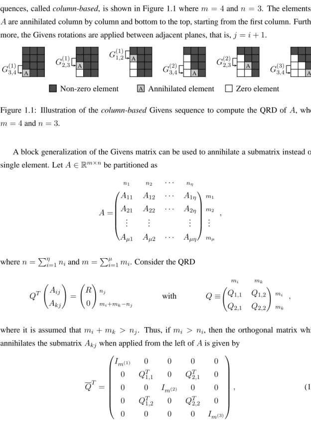
A sequence of Givens rotations can be applied to compute the QRD (1.4). One of such se-quences, called column-based, is shown in Figure 1.1 where m = 4andn = 3. The elements of Aare annihilated column by column and bottom to the top, starting from the first column. Further-more, the Givens rotations are applied between adjacent planes, that is,j =i+ 1.

A G(1)₃_,₄ G A (1) 2,3 A G(1)₁_,₂ A G(2)₃_,₄ G A (2) 2,3 A G(3)₃_,₄ Non-zero element A _{Annihilated element} _{Zero element}

Figure 1.1: Illustration of the column-based Givens sequence to compute the QRD of A, where m= 4andn= 3.

A block generalization of the Givens matrix can be used to annihilate a submatrix instead of a single element. LetA_∈Rm×nbe partitioned as

A= n1 n2 · · · nη             A11 A12 · · · A1η m1 A21 A22 · · · A2η m2 .. . ... ... ... Aµ1 Aµ2 · · · Aµη mµ ,

wheren=Pη_i₌₁niandm=Pµ_i₌₁mi. Consider the QRD

QT Aij Akj ! = R 0 ! nj mi+mk−nj with Q_≡ mi mk ! Q1,1 Q1,2 mi Q2,1 Q2,2 mk ,

where it is assumed that mi +mk > nj. Thus, if mi > ni, then the orthogonal matrix which

annihilates the submatrixAkj when applied from the left ofAis given by

QT =          I_m(1) 0 0 0 0 0 QT₁_,₁ 0 QT₂_,₁ 0 0 0 I_m(2) 0 0 0 QT₁_,₂ 0 QT₂_,₂ 0 0 0 0 0 I_m(3)          , (1.6)

(21)

1.3. GENERALIZED QR DECOMPOSITION AND THE GENERAL LINEAR MODEL 7 wherem(1)₌_m

1+m2+· · ·+mi−1,m(2)=mi+1+mi+2+· · ·+mk−1andm(3)=mk+1+

mk+2+· · ·+mη. Notice that in generalQis not a rotation matrix. The orthogonal matrices having

the form ofQin (1.6) are extensively used in this treatment to develop strategies which exploit the sparse block-structure of the various matrices which arise in the estimation of econometric linear models [20, 24, 25, 22, 46].

1.3 Generalized QR Decomposition and the General Linear Model

The variance-covariance matrix of the disturbances Ω of the GLM (1.2) is often assumed to be positive definite. In such cases the BLUE ofβin (1.2) comes from solving the Generalized Least Squares (GLS) problem

argmin β

y₋Xβ_Ω−1 which is equivalent to the normal equations

XTΩ−1Xβ=XTΩ−1y. (1.7)

This solution, however, can be unstable when the matrices are ill-conditioned and explicit matrix inversion are used [9, 57]. Furthermore, ifΩis singular, then the GLS estimator cannot be com-puted using (1.7) and the replacement ofΩ−1by the Moore-Penrose generalized inverse would not always give the BLUE ofβ[55].

To avoid problems associated with the singularity or ill-conditioning ofΩ, the GLM (1.2) can be formulated as the Generalized Linear Least Squares Problem (GLLSP)

argmin υ,β

υTυ subject to y=Xβ+Cυ, (1.8)

whereΩ _∈ Rm×m is non-negative definite with rankg,Ω = CCT,C _∈ Rm×g has full column rank, the randomg-element vectorυis defined asCυ=ε. That is,υ _∼(0, σ2_I

g)[55]. The

Gen-eralized QRD (GQRD) can be employed to solve GLLSP [2, 64]. Although the above formulation allows for singular Ω, without loss of generality consider the case whereΩis non-singular. The GQRD ofX andCis given by the QRD (1.4) and the RQD ofQT_C_{which can be written as}

(QTC)P =U _≡ n m−n ! U11 U12 n 0 U22 m−n , (1.9)

(22)

whereP _∈Rm×mis orthogonal andU _∈Rm×mis upper triangular and non-singular. The GLLSP (1.8) can be equivalently written as

argmin υ,β PTυ2 subject to QTy=QTXβ+QTCP PTυ or argmin υ1,υ2,β υ1 2 +υ2 2 subject to    y1 =Rβ+U11υ1+U12υ2, y2 =U22υ2, (1.10)

whereυT_P _{is conformably partitioned as}₍_υT

1 υ2T). In the second constraint of (1.10)υ2 comes

from solving the upper triangular system U22υ2 = y2, and in the first constraint the arbitrary

subvector υ1 is set to zero in order to minimize the objective function. Thus, the estimator ofβ

derives from the solution of the upper triangular systemRβ=y1−U12υ2. The variance-covariance

of the coefficients estimator is given by σˆ2R−1U11U11TR−T, where σˆ2 = υ2Tυ2/(m−n) is an

estimator ofσ2_.

1.4 The SUR model

The SUR model is a special case of the GLM. It is defined by the set of regressions yi =Xiβi+ui, i= 1, . . . , G,

whereXi ∈RT×kihas full column rank,yi∈RT and theT-element disturbance vectoruihas zero

mean, variance-covariance matrixσi,iIT and is contemporaneously correlated across the equations,

soE(uiuTj) =σi,jIT. In compact form the SUR model is written

       y1 y2 .. . yG        =        X1 0 · · · 0 0 X2 · · · 0 .. . ... . .. ... 0 0 _{· · ·} XG               β1 β2 .. . βG        +        u1 u2 .. . uG        or

Vec(Y) = _⊕G_i₌₁XiVec({βi}G) + Vec(U), (1.11)

where Y = y1. . . yG ∈ RT×G, ⊕Gi=1Xi = diag(X1, . . . , XG) ∈ RT×K denotes the direct

(23)

1.4. THE SUR MODEL 9 The disturbance termVec(U)has zero mean and variance-covariance matrixΣ_⊗IT, whereΣ = [σi,j]∈ RG×G is symmetric and non-negative definite and⊗denotes the Kronecker product [42,

50, 51, 70, 73, 78, 79, 86, 87]. That is,Vec(U)_∼(0,Σ_⊗IT)and

Σ_⊗IT =        σ1,1IT σ1,2IT · · · σ1,GIT σ2,1IT σ2,2IT · · · σ2,GIT .. . ... ... σG,1IT σG,2IT · · · σG,GIT       

Notice that(A_⊗B)(C_⊗D) =AC_⊗BDandVec(ABC) = (CT _⊗_A_{) Vec(}_B₎_.

The solution of the GLLSP (1.8) has also been discussed within the context of estimating SUR models and their variants [6, 14, 34, 52, 56, 71, 89]. This formulation and the use of the GQRD allows to desing computationally efficient methods by exploiting the special structure of the regressor and covariance matrices.

Often in econometric special cases or extensions of the SUR model are considered. The most common cases are here briefly reviewed:

• Heteroschedastic disturbances. In this extension the assumption of a spherical distributed

uiis relaxed. The covariance matrix ofuianduj is assumed to beE(uiuTj) =σi,jD, where

Dis a diagonal matrix of positive elements. Thus, the variance-covariance matrix ofVec(U)

is given byΣ_⊗D.

• Correlation Constraints. SUR models where the disturbances covariances are constrained

includes the SUR model with Correlation Constrains (SUR-CC) [48, 79, 88]. In this models the elements of the covariance matrix is constrained so that the variance of one disturbance is smaller than that of the disturbance in the successive equation. Furthermore, the correlation between the disturbances are between zero and one. That is,

σ1,1 ≤σ2,2 ≤ · · · ≤σG,G

and

0< ρi,j <1, i, j= 1, . . . , Gandi6=j,

whereρi,j = σi,j/√σi,iσj,j is the correlation betweenui,tand uj,t. This specification has

applications in the context of error components models, where the disturbance term is de-fined asui =Pij=1εj,εi∼(0, υiIT)andE(εiεTj) = 0fori6=j.

(24)

• Autoregressive disturbances. In the SUR model (1.11) the disturbances are assumed to

be uncorrelated across time. However, in several applications this is to much restrictive and correlation on time should be considered. In the SUR model with autoregressive (AR) disturbances, hereafter SUR-AR model, the errors are generated by the AR process

ui,t=αiui,t−1+εi,t, i= 1, . . . , G, t= 2, . . . , T,

and whereαiare the AR parameters, εi,t ∼ (0, σi,i),E(εi,tεj,t) =σi,j andE(εi,sεj,t) = 0

for s ₆= t and i, j = 1, . . . , G [26, 43, 65, 85]. This can be written in compact form as ui=αiZui+εi (i= 1, . . . , G), or

Vec(U) = (_⊕iαiZ) Vec(U) + Vec(E), Vec(E)∼(0,Σ⊗IT),

whereεi = εi,1 · · · εi,T

T

,E = ε1 · · · εG

andZdenotes theT _×T shift matrix

          0 0 _{· · ·} 0 0 1 0 _{· · ·} 0 0 0 1 _{· · ·} 0 0 .. . ... . .. ... ... 0 0 _{· · ·} 1 0           .

In this model the covariance matrix ofVec(U)is given by

⊕Gi=1(IT −αiZ)−1 Σ⊗IT ⊕Gi=1(IT −αiZ)−T

• Vector Autoregressive disturbances. A more general form of autocorrelation is given by

the Vector Autoregressive (VAR) process:

U =ZU AT +E, Vec(E)_∼(0,Σ_⊗IT),

whereA_∈RG×Gis the matrix of the AR parameters. In this case the covariance matrix of the SUR disturbances is given by

IGT −A⊗Z−1 Σ⊗IT IGT −A⊗Z−T.

Additional assumption regarding the disturbances of the first observation, that is ui,1 (i =

(25)

1.4. THE SUR MODEL 11 to include more that one lags in the autoregressive specification, that is the disturbances are follow the VAR(p) process

U =ZU AT₁ +Z2U AT₂ +_{· · ·}+ZpU AT_p +E, Vec(E)_∼(0,Σ_⊗IT),

whereA1, . . . , Ap ∈RG×Gare the matrices of the AR parameters.

• Unequal Size Observations. The formulation of the SUR model, as given in (1.11), assumes

that each regression has the same number of observations, however this might not always be the case [72, 74, 77, 79]. The SUR model with Unequal Size Observation (SUR-USO) assumes that the ith equation has ti observations and that the first ti observations for the (i+1)th regression match in time with those for theith regression. In this case the covariance matrices of the disturbancesuianduj, forj > iare given by

E(uiuTj) =σi,j

Iti 0ti×(tj−ti)

.

• Missing Observations. A generalization of the SUR-USO model, is given by the SUR

model with Missing Observations. There, the pattern of the observations which are missing is not fixed and the ti observations of theith equation does not necessarily match in time

with the first of(i₋1)th regression. The covariances in this case are given by

E(uiuTj) =σi,jSi,j,

whereSi,j isti×tj zero-one matrix with its(k, l)element being non zero if thekth andlth

observations of theith andjth equations, respectively, match in time.

• Common Regressors. In the SUR model with Common Regressors, the exogenous matrix

Xi = XdSi (i = 1, . . . , G), where Xd ∈ RT×k

d

denotes the matrix consisting of the Kd distint regressors andSi∈RK

d_×_k

i _{is a selection matrix that comprises the relevant columns} of the Kd_×Kd identity matrix. This is often the case because an exogenous factor can appear in more than one regressor matrix. For example such occurs when estimating the multivariate linear regression model

Y =XdB+U, Vec(U)_∼(0,Σ_⊗IT),

with the constraints

(26)

That is, nelements of the parameter matrixB _∈ RKd×G are restricted to zero, or, equiv-alently, the isth column of Xd is not included in the model to predict thejsth column of

Y.

• Triangular SUR models. Triangular SUR models are special cases of SUR models with

common regressor. In these models, the equations and the columns of each exogenous ma-trix can be reordered such that the ith regressor consists of a subset of the columns of the following one, that is,Xi= Xi−1 Xei

, whereXei∈RT×ki−ki−1.

1.5 Overview of the thesis

Each chapter of the thesis is self contained1. Chapter 2 considers the estimation of Vector Au-toregressive (VAR) processes with zero coefficient constraints. This estimation problem reduces to that of estimating a SUR model with common regressors, where the matrix of distinct regressors Xd has block Toeplitz structure. The analysis presented is extended to the VARX model, where exogenous factors, such as linear or polynomial trends in the data generation process, are included into the model. A procedure is detailed for reducing the size of model by efficiently computing the triangular R-factor in the QRD of the exogenous matrixXd. Then the estimation of SUR models with common regressors and that of the triangular SUR models are considered. These model derive from the estimation of VAR models with zero coefficient constraints or VAR model with Granger (non-causality) restrictions, respectively. This analysis extends the one that have been provided in [51] where a specific ordering on the equations was imposed and applies to situations where different Granger causality restrictions need to be imposed and tested.

In Chapter 3 methods for estimating the SUR model with AR and VAR disturbances (SUR-VAR) are presented. In that model the covariance matrix of the disturbances is dense and structured. When the number of observations is large the SUR-VAR model can be reduced to a GLM of smaller dimensions. Efficient strategies to solve the resulting GLLSP which exploit the structure of the Cholesky factor of the covariance matrix are derived.

The estimation of the SUR model Unequal Size Observations (SUR-USO) is considered in Chapter 4. Two algorithms which solve the GLLSP derived from the SUR-USO model are pro-posed. The first computes the GQRD of the regressor and Cholesky factor of the dispersion matrix. While, the second use a recursive approach to solve the GLLSP, where at each step a set of

obser-1

(27)

1.5. OVERVIEW OF THE THESIS 13 vations are added to the model. Furthermore, an estimator for the covariance matrix is proposed for the case of normally distributed disturbances. With respect to most of the existing estimators, this has the advantage of being always non-negative definite.

Chapter 5 presents existing direct methods for estimating the basic SUR model and proposes two new methods. The first is based on a recursive approach, while the second on the transforma-tion of the SUR model to a smaller SUR-USO model. The derivatransforma-tion of the algorthms is presented and their comparison based on their theoretical complexity and on computational experiments is given. Finally, the last chapter concludes and provides directions for future research.

(28)

(29)

Chapter 2

Estimation of VAR models

Abstract:

The Vector Autoregressive (VAR) model with zero coefficient restrictions can be formulated as a Seemingly Unrelated Regression Equations (SURE) model. Both the response vectors and the coefficient matrix of the regression equations comprise columns from a Toeplitz matrix. Efficient numerical and computational methods which exploit the Toeplitz and Kronecker product structure of the matrices are proposed. The methods are also adapted to provide numerically stable algo-rithms for the estimation of VAR(p) models with Granger–caused variables.

2.1 Introduction

The vector time serieszt∈Rnis a Vector Autoregressive (VAR) process of orderpwhen its data

generation process has the form

zt= Φ1zt−1+ Φ2zt−2+· · ·+ Φpzt−p+ut, (2.1)

whereΦi ∈ Rn×n are the coefficient matrices and the vectorsut ∈ Rn are serially uncorrelated

and identically distributed with zero mean and variance–covariance matrixΣ. That is,E(ut) = 0,

E(utuTt) = ΣandE(utuTτ) = 0, fort6=τ.

1

This chapter is a reprint of the paper: P. Foschi, E.J. Kontoghiorghes. Estimation of VAR models: computational aspects. Computational Economics, 21(1):3-22, 2003.

(30)

Given a sample z1, . . . , zM and a presample z1−p, . . . , z0 the VAR model (2.1) is efficiently

estimated by Ordinary Least Squares (OLS) estimation of the model

       z_MT zT M−1 .. . zT 1        =        z_MT ₋_p z_MT ₊₁₋_p _{· · ·} z_MT ₋₁ zT M−1−p zMT −p · · · zMT −2 .. . ... ... zT 1−p zT2−p · · · z0T               ΦT_p ΦT p−1 .. . ΦT 1        +        uT_M uT M−1 .. . uT 1        ,

which in compact form it can be written as

Y =XB+U, (2.2)

where Y, X, B and U are defined by the context. The variance–covariance matrix of Vec(U)

is Σ_⊗IM, whereVec(·) denotes the column stacking operator and ⊗is the Kronecker product

operator. The OLS and Generalized Least Squares (GLS) estimators of (2.2) are the same [58, 86]. LetT = X Yand its QR decomposition (QRD) be given by

T =Q R 0 ! = np n M−(p+1)n QT QY QN np p       RT RT Y np 0 RY p 0 0 M−(p+1)n , (2.3)

whereQ_∈RM×M is orthogonal andR_∈R(n+1)p×(n+1)pis upper triangular. The OLS estimator ofBin (2.2) is computed by

ˆ

B =R−_T1RT Y.

The residuals are given by

ˆ

U =QYRY,

and the covariance matrixΣis estimated by

ˆ

Σ =αUˆTUˆ =αR_YTRY,

whereα= 1/M orα= 1/(M ₋np).

AlternativelyR in (2.3) may be computed using the Cholesky factorization of TTT, but this is neither computationally efficient nor numerically stable due to the poor numerical properties of the matrixTTT. Efficient methods avoid this problem by computing the Cholesky factorization without forming that matrix explicitly.

(31)

2.1. INTRODUCTION 17 The matrix T is Block-Toeplitz with blocks of size 1_×nthat are constant along the diago-nals. Exploiting the structure ofT, a fast algorithm is possible for computing the upper triangular matrices in (2.3) and, thus, a fast estimation algorithm can be designed.

When other, possibly endogenous, factors such as deterministic trends are added, (2.1) becomes zt= Θwt+ Φ1zt−1+ Φ2zt−2+· · ·+ Φpzt−p+ut, (2.4)

where wt ∈ Rη and Θ ∈ Rn×η. The OLS estimates of (2.4) can be computed the same way as

those of (2.1). However, care must be taken in arranging the matrix of regressors (endogenous and exogenous) in (2.3) to minimize the loss of structure derived from the introduction of the endogenous variableswt. A good choice isM = W X Y

, whereWT = wM wM−1 · · · w1

. The complexity of the algorithms will be given in flops (floating point operations per second), where flop denotes a single scalar multiplication or addition. Throughout the paper, the following notation is used: the vectoreidenotes theith column of then×nidentity matrixInand then×n

shift matrix is denoted byZ = (e2 e3 · · · en0), that is

Z=           0 0 _{· · ·} 0 0 1 0 _{· · ·} 0 0 0 1 _{· · ·} 0 0 .. . ... . .. ... ... 0 0 _{· · ·} 1 0           .

A set of vectors v1, v2, . . . , vnis denoted by{vi}nand the direct sums of two or more matrices

A_⊕Band_⊕n_i₌₁Aiare equivalent to the block diagonal matrices

A 0 0 B ! and        A1 0 · · · 0 0 A2 · · · 0 .. . ... . .. ... 0 0 _{· · ·} An        ,

respectively [3, 30, 69]. For notational convenience the subscript n in the set operator _{·}n is

dropped and_⊕n_i₌₁will be abbreviated to_⊕i.

The purpose of this work is twofold. First, to exploit the structure of the Toeplitz matrix in (2.2) and provide a fast algorithm to compute the upper triangular matrixRand, consequently, an efficient estimation procedure for the VAR(p) models. Second, to design computationally efficient

(32)

methods to estimate VAR models with coefficient constraints by exploiting the Kronecker product structure of the Seemingly Unrelated Regression Equations (SURE) models.

In section 2.2 the Generalized Schur Algorithm (GSA) and its block version are presented. In section 2.3 the adaption of the algorithm to estimate the VAR models (2.1) and (2.4) is considered. In section 2.4 the estimation of the VAR model with Zero Coefficient Constraints (VAR-ZCC) and the resulting SURE model are investigated. Finally in section 2.5 the estimation of the VAR model with Granger–causality restrictions is presented. This model is considered as a SURE model with Proper Subset Regressors (SURE-PSS).

2.2 Structured matrices and the Generalized Schur Algorithm

LetA _∈ Rn×n be a positive definite matrix andF _∈ Rn×n be strictly lower triangular; that is, F = [fij]withfij = 0fori≤j. The displacement ofAwith respect to (w.r.t.)F is

∇FA=A−F AFT (2.5)

and its rankd= rank(_∇FA)is called the displacement rank ofA. The matrixAis said to have a

displacement structure or, more simply, be structured w.r.t. F if it has a small displacement rank. In this case

∇FA=GTJG, (2.6)

whereG_∈ Rd×n,J =Ik⊕(−Il)andk+l =d. The rows ofGare called the generators ofA

[39, 40].

Given F, the matrix A is uniquely defined by k, l and G. In fact, since F is strictly lower triangular,Fn_{= 0}_{, and from (2.5) and (2.6) it follows that}

A= n−1 X i=0 Fi(A₋F AFT)(Fi)T = n_X−1 i=0 FiGTJG(Fi)T, (2.7)

where it has been assumedF0=In. Consider for example the symmetric Toeplitz matrix

T =           t1 t2 t3 · · · tn t2 t1 t2 · · · tn−1 t3 t2 t1 · · · tn−2 .. . ... ... . .. ... tn tn−1 tn−2 · · · t1           .

(33)

2.2. STRUCTURED MATRICES AND THE GENERALIZED SCHUR ALGORITHM 19 This is a structured matrix and its displacement rank w.r.t. the shift matrixF = e2 e3 · · · en0

– the matrix with ones on the first sub-diagonal and zero elsewhere – is 2, k = l = 1, and the generators are G= √1 t1 t1 t2 t3 · · · tn 0 t2 t3 · · · tn ! .

A Generalized Schur Algorithm (GSA) can be used to compute the

Cholesky factorization A = RTR when A has displacement structure (2.6). At each iteration a row ofR is computed. Since the first column ofFi_G_{is zero for}_i_≥ ₁_{, it follows from (2.7) that}

the first row ofAis given by

a11 a12 · · · a1n = r11 r11 r12 · · · r1n = g11 g21 · · · gd1 JG. (2.8)

IfQis aJ-invariant matrix (a hyperbolic transformation), that isQJQT =J, then the rows of

˜

G=QT_G_{are again generators for}_A_{. If}_Q_{is chosen to annihilate the first column of}_G_{except for}

the(1,1)–element, then (2.8) is given by

˜ g11 ˜ g11 g˜12 · · · g˜1n ; that is,g˜T₁ = ˜g11 ˜g1n · · · ˜g1n

is the first row ofR. Consider now the partitioning

R= i−1 n−i+1 ! R1 R12 i−1 0 R2 n−i+1 , A= i−1 n−i+1 ! A11 A12 i−1 A21 A22 n−i+1 and define A(i)=A₋ R T 1 RT₁₂ ! R1 R12 = 0 0 0 S ! ,

whereS =RT₂R2is the Schur complement ofA11. IfA(i)has displacement structure

∇FA(i)=GTi JGi , (2.9) with Gi = i−1 1 n−i ! 0 u1 uT2 1 0 v1 V2 d−1 , (2.10)

(34)

andQiis aJ-invariant matrix that annihilates the elements ofv1, that is, ˜ Gi =QTi Gi= i−1 1 n−i ! 0 ρ u˜T 1 0 0 V˜ d−1 , (2.11)

then the first row ofR2 is given by ρu˜T. Now, ifriT = 0T ρ u˜T

, thenA(i+1) =A(i)₋ririT,

which has displacement given by

∇FA(i+1) = GTi JGi−ririT +F ririTFT = G˜T_i JG˜i−ririT +F ririTFT = GT_i₊₁JGi+1, where Gi+1 = rT_i FT 0(r−1)×i V˜ ! (2.12) has the same structure as (2.10), i.e., the firstielements ofF riare zero. Thus, given the generators

ofAin (2.6), the rows of the Cholesky factorRcan be computed by iterating equations (2.11) and (2.12). The algorithm may breakdown if

uT₁ vT₁ J u1 v1 ! <0.

At each step of the algorithm, aJ-invariant matrixQi should be computed to annihilate the

elements ofv1in (2.10). The computation of this matrix plays a key role in the numerical stability

of the whole algorithm [81]. In particular the number of hyperbolic transformations should be minimized. Here only one hyperbolic Givens rotation is used and this is in factored form [81].

Let (xT yT) = (uT₁ v₁T), where x _∈ Rk and y _∈ Rl. If Qx ∈ Rk×k and Qy ∈ Rl×l

are two orthogonal matrices, then Qx ⊕Qy is J-invariant. If Qx and Qy are the Householder

transformations such thatQT_xx=αe1andQTyy=βe1, andH∈R2×2is such that

H α β ! = ρ 0 ! and HT 1 0 0 ₋1 ! H= 1 0 0 ₋1 ! ,

(35)

2.2. STRUCTURED MATRICES AND THE GENERALIZED SCHUR ALGORITHM 21 then the matrix

Q= Qx 0 0 Qy !        h11 0 h12 0 0 Ik−1 0 0 h21 0 h22 0 0 0 0 Il−1       

isJ-invariant and satisfies

QT x

y

!

=ρe1.

Notice that if no breakdown occurs, then the matrixH can be always computed as the hyperbolic Givens rotation H= 1 c 1 s s 1 ! ,

wheres=₋β/αandc2 = 1₋s2. In factored form this is

H = 1 0 s c ! 1/c 0 0 1 ! 1 s 0 1 ! ,

which represents a stable implementation of the transformation H

[81].

Algorithm 1 summarizes the Generalized Schur Algorithm. It needs to store only the generators Giand the matrixR; the matrixA(i)is never computed explicitly. Supposing that the matrix–vector

multiplication involvingF is negligible (whenF is a shift matrix) and using Householder matrices forQx andQy, the computational cost of the algorithm is dominated by the steps 5 and 7, which

require4d(n₋i)and6(n₋i)flops, respectively [28]. Therefore, the complexity of the algorithm is(2d+ 3)n2.

For some applications a block version of the algorithm is more appropriate. That is, ifA, F _∈ RN n×N n are matrices with block–size n_×n, then F is block strictly lower triangular and A has displacement rank d w.r.t. F. A possible implementation of the Block Generalized Schur Algorithm (BGSA) is outlined in Algorithm 2. Steps 4–7 compute aJ-invariant transformationQi

such that QT_i X1 Y1 ! = Ri 0 ! . (2.13)

Notice that other implementations exist for computing (2.13) each of which has different numerical properties. In Algorithm 2 the only critical part, concerning numerical stability, is the computation

(36)

Algorithm 1 Generalized Schur Algorithm

Input: The matrix of generatorsGand the shift matrixFas in (2.5) and (2.6)

Output: R, the upper triangular Cholesky factor ofA

1: SetG(1)=G 2: fori= 1,2, . . . , n−1do 3: Let G(i)= i−1 1 n−i ! 0 x X k 0 y Y l .

4: Compute the Householder reflectionsQxandQysuch thatQTxx=αe1andQTyy=βe1, respectively.

5: ApplyQxandQytoXandY, respectively, such that:

˜

X =QTxX, Y˜=Q T yY.

6: Compute a hyperbolic Givens transformationHsuch that

HT α β

!

=ρe1.

7: ApplyHto the first rows ofX˜andY˜to obtainXˆ,Yˆ and

ˆ G(i)= 0 ρe1 Xˆ 0 0 Yˆ ! .

8: Store(0 · · · 0 ρ Xeˆ 1)in theith row ofR.

9: G(i+1)is defined byGˆ(i)after its first row has been multiplied byF.

10: end for

of the hyperbolic transformationHin Step 6. The breakdown of the block algorithm [27] is related to the non-existence or the singularity ofRiin (2.13).

If Householder transformations are used, then the computational complexity of Steps 4 and 5 is

4n2(N₋i)(d₋n)flops. The number of flops for Steps 6 and 7 using hyperbolic Givens rotations is given by n X j=1 j X h=1 6((N ₋i)n+h) _' n X j=1 6(j(N ₋i)n+1 2j 2₎ ' 4(N ₋i)n3.

(37)

2.2. STRUCTURED MATRICES AND THE GENERALIZED SCHUR ALGORITHM 23

Algorithm 2 Generalized Schur Algorithm – Block Version Input: The matrix of generatorsGand the shift matrixFas in (2.5) and (2.6)

Output: R, the upper triangular Cholesky factor ofA

1: LetG(1)=GandJ=Ik⊕ −Il. 2: fori= 1,2, . . . , Ndo 3: Let Gi= (i−1)n n (N−i)n „ ₀ _X « 1 X2 k 0 Y1 Y2 l . 4: Compute the QRDs X1=QX RX 0 ! and Y1=QY RY 0 ! . 5: Compute n k−n ˆ X2A ˆ X2B ! =QTXX2 and n l−n ˆ Y2A ˆ Y2B ! =QTYY2.

6: Compute a J-invariant matrixHsuch that

HT RX RY ! = Ri 0 ! . 7: Compute ˇ X2A ˇ Y2B ! =HT X_ˆˆ2A Y2B ! .

8: Store`0RiXˇ2A´in theith block–row ofR.

9: Compute in (N−i)n ` ´ 0 XˆA = (i−1)n n (N−i)n ` ´ 0 Ri Xˇ2A FT

and formGi+1as:

Gi+1= (i−1)n n (N−i)n 0 B B @ 1 C C A 0 0 XˆA n 0 0 X˜2B k−n 0 0 Yˇ2A n 0 0 Y˜2B l−n . 10: end for

Thus, the computational complexity of the whole procedure is given by

N X i=1 (N ₋i)n2(4n+ 4(d₋n)) _' N X i=1 4d(N ₋i)n2 ' 2dN2n2.

(38)

2.3 A fast algorithm for the OLS estimation of the VAR model

The BGSA shown by Algorithm 2 is designed to compute the Cholesky factorization of structured matrices. To compute the matrix R in (2.3) the algorithm should be applied to the matrixTTT. Consider the block Toeplitz matrixT _∈RM m×N ndefined by

T = [Ti−j]ji=1=1,...,M,...,N, that is, T =        T0 T−1 · · · T1−N T1 T0 · · · T2−N .. . ... ... TM−1 TM−2 · · · TM−N        , (2.14)

whereTk∈Rm×n. LetA=TTT, where the(i, j)th blockAij ∈Rm×nis given by

Aij = M X k=1 T_kT₋_iTk−j =YiT−1Yj−1 andYT i = T−TiT1T−i · · · TMT−i−1

is the(i+ 1)th block column ofT. IfY0has full column rank,

then the displacement rank ofAw.r.t.Zm=Z⊗Imis2(m+n)and the generators (see Appendix

1) are given byJ =Im+n⊕ −Im+nand

G= n n · · · n             R0 QT0Y1 · · · QT0YN−1 n 0 T−1 · · · T1−N m 0 QT₀Y1 · · · QT0YN−1 n 0 TM−1 · · · TM+1−N m , (2.15)

whereY0=Q0R0,R0 ∈Rn×nis upper triangular andQ0∈RM m×nis orthogonal.

IfM = W T, whereW _∈RM m×η, then the displacement equation forA¯ = MTM w.r.t. the shift matrixZ¯= 0η×η ⊕Zmis

∇_Z¯A¯= 0 0 0 _∇ZmTTT ! + W T_W _WT_T TT_W ₀ ! ,

(39)

2.4. VAR MODELS WITH ZERO COEFFICIENT CONSTRAINTS 25 so that the generators are given byJ =Iη+m+n⊕ −Iη+m+nand

G= η n n · · · n                       RW QTWY0 QTWY1 · · · QTWYN−1 η 0 R0 QT0Y1 · · · QT0YN−1 n 0 0 T−1 · · · T1−N m 0 QT WY0 QTWY1 · · · QTWYN−1 η 0 0 QT 0Y1 · · · QT0YN−1 n 0 0 TM−1 · · · TM+1−n m . (2.16)

The computational complexity of (2.16) can be approximated by4n2((n+mM/2)N+η). Notice that if the generators are given by (2.15), or by (2.16), then Steps 4–7 of Algorithm 2 are not needed for the first iteration.

In the specific case of the estimation of VAR modelsm = 1, N = p+ 1, Tk = yTM−N−k,

Y_iT = yM+i−p · · · y2+i−p y1+i−p and the displacement rank ofA and A¯are 2(n+ 1)and 2(n+η+ 1), respectively. Thus, the computation of the Cholesky decomposition ofA¯TA¯using Algorithm 2 requires2(n+η)n2p2flops, and the computation of the generators requires a further

4n2₍₍_n₊_M/₂₎_p₊_η₎_flops.

2.4 VAR models with Zero Coefficient Constraints

The VAR model (2.2) can be written as the SURE model

Vec(Y) = (In⊗X) Vec(B) + Vec(U),

whereVec(U)has zero mean and variance–covariance matrix given byΣ_⊗IM. Often zero

coeffi-cient constraints (ZCC) are imposed to VAR models, hereafter called VAR-ZCC model [58]. Thus, some elements ofBare zero. Letβi∈Rki the vector of nonzero elements in theith column ofB.

The VAR-ZCC model can be written as the SURE model

Vec(Y) = (_⊕n_i₌₁Xi) Vec({βi}n) + Vec(U), (2.17)

whereXi =XSiandSi ∈Rnp×kiis a selection matrix. Notice that the SURE model has common

(40)

The Best Linear Unbiased Estimator (BLUE) ofVec(_{βi})is obtained from the solution of the

General Least Squares (GLS) problem

argmin β1,...,βn Vec(Y)₋Vec(_{Xiβi}) Σ−1_⊗_I_M (2.18) which is given by Vec(_{βˆi}) = (⊕iXiT)(Σ−1⊗IM)(⊕iXi) −1 (_⊕iXiT) Vec(YΣ−1). (2.19)

The computation of (2.19) has poor numerical properties and does not allow for a singular dis-persion matrixΣ. Therefore, it is preferable to formulate (2.18) as the Generalized Linear Least Squares Problem (GLLSP)

argmin V,{βi}

V_F subject to Vec(Y) = (_⊕iXi) Vec({βi}) + Vec(V CT), (2.20)

where_k·kF denotes the Frobenious norm,Σ =CCT, the upper triangularC∈Rn×nhas full rank

and the random matrixV is defined as(C_⊗IM) Vec(V) = Vec(U). That is,V CT =U, which

implies thatVec(V)has zero mean and variance-covariance matrixInM [50, 55, 61, 63]. Without

loss of generality it will be assumed thatΣis non-singular. Consider the Generalized QR decomposition (GQRD)

QT (_⊕iXi) = ⊕i Ri 0 ! (2.21a) and QT(C_⊗IM)P = K nM−K ! W11 W12 K 0 W22 nM−K , (2.21b)

where K = Pn_i₌₁ki, Ri ∈ <ki×ki and W22 are upper triangular, and Q,P ∈ RnM×nM are

orthogonal [2, 64]. Using (2.21) the GLLSP (2.20) can be written as

argmin {viA}, {viB},{βi} G X i=1 kviAk2+kviBk2 subject to Vec (_{yiA}) Vec (_{yiB}) ! = ⊕iRi 0 ! Vec(_{βi}) + W11 W12 0 W22 ! Vec (_{viA}) Vec (_{viB}) ! , (2.22)

(41)

2.4. VAR MODELS WITH ZERO COEFFICIENT CONSTRAINTS 27 where QTVec(Y) = Vec ({yiA}) Vec (_{yiB}) ! K nM−K and PT Vec(V) = Vec ({viA}) Vec (_{viB}) ! K nM−K .

From (2.22) it follows that Vec (_{viB}) = W22−1Vec ({byi}) and Vec ({viA}) = 0. Thus, the

solution for the SURE model comes from solving the triangular system

Vec (_{yiA}) Vec (_{yiB}) ! = ⊕iRi W12 0 W22 ! Vec(_{βi}) Vec (_{viB}) ! . (2.23)

The matrix_Qin (2.21) is defined as

Q=_⊕_iQiA ⊕iQiB , where QT_i Xi = Ri 0 ! , with Qi = ki M−ki QiA QiB , is the QRD ofXi(i= 1, . . . , G).

The computation of (2.21b) occurs in two stages. The first stage computes

QT(C_⊗I)_Q= K nM−K ! f W11 Wf12 K f W21 Wf22 nM−K , (2.24)

whereW˜ij (i, j = 1,2) is block upper triangular. Furthermore, the main block–diagonals ofW˜12

andW˜21are zero, and theith (i= 1, . . . , G) blocks of the main diagonal ofW˜11andW˜22are given

byCiiIkiandCiiIM−ki, respectively. The second stage computes the RQD

f W21 fW22 e P =0 W22 (2.25a) and f W11 fW12 e P =W11 W12 . (2.25b)

(42)

Thus, in (2.21b)_P =_Q_P˜. Sequential and parallel strategies for computing the RQD (2.25) have been described in [44, 46].

The computations of (2.24) and (2.25) are the most expensive operations – their computational cost is in the order ofn3M3– and they become quite important when computing the feasible GLS (FGLS) estimators, that is, when computed at each iteration for differentC. However, the common regressors that exist in the SURE model can be used to reduce the computational complexity of the iterative estimation procedure [54].

Consider the QRD given in (2.3). Premultiplying (2.17) from the left by

¯ QT = In⊗QT In⊗QY In⊗QNT gives     Vec(RT Y) Vec(RY) 0    =     ⊕iRSi 0 0    Vec({βi}) +     Vec(UT) Vec(UY) Vec(UN)    , where QTU = n       UT np UY n UN M−(p+1)n .

The covariance matrix ofVec( UT UY UN)is given by

    Σ_⊗Inp 0 0 0 Σ_⊗In 0 0 0 Σ_⊗IM−n(p+1)    .

Thus the estimator of the SURE model (2.17) arises from the solution of the reduced size model

Vec(RT Y) = (⊕iRTSi) Vec({βi}) + Vec(UT), (2.26)

where the covariance matrix ofVec(UM)is given byΣ⊗Inp. The estimator ofΣis now given by ˆ Σ = 1 M ˆ U_TTUˆT +RTYRY ,

whereUˆ is the residual matrix estimated from (2.26). Notice thatRT_YRY does not depend on the

(43)

2.5. VAR MODELS WITH GRANGER CAUSALITY RESTRICTIONS 29

2.5 VAR models with Granger causality restrictions

Consider partitioning the time seriesztand the coefficient matricesΦlin (2.1) as

zt= zAt zBt ! Φl = ΦAAl ΦABl ΦBAl ΦBBl ! .

IfΦBAl = 0forl= 1,2, . . . , p, then the serieszAtdoes not Granger–causezBt; that is,zAtis not

linearly informative about the future of the time serieszBt[32, 58]. This concept can be

general-ized. Define the permutation(π1, . . . , πn)of the indices(1, . . . , n), and letΠ = eπ1 eπ2 · · · eπn

be the associated permutation matrix. Now, if there exists a permutation(π1, . . . , πn)such that

ΠTΦlΠ∼ h1 h2 · · · hs             × × · · · × k1 0 _{× · · · ×} k2 .. . ... . .. ... ... 0 0 _{· · · ×} ks , (2.27)

forl= 1,2, . . . , p, then the serieszπjdoes not Granger–causezπlwhen the(i, j)th element of the matrix in (2.27) belongs to the block lower triangular part.

When the Granger causality restrictions are known a priori, the variables can be ordered so that the matricesΦlhave the structure given in (2.27). In this case the model is equivalent to a triangular

SURE model [79, 51]. Conversely, if different models with different causality restriction have to be estimated, then a reordering is not convenient since the Toeplitz structure ofXis destroyed. In this case the VAR model is equivalent to a SURE model with proper subset regressors [79].

Multiplying (2.2) on the right byΠgives

˜

Y =XB˜+ ˜U ,

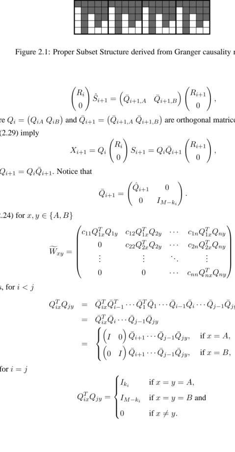
whereY˜ =YΠ,U˜ =UΠandB˜ =BΠ. Figure 2.1 shows an example of the structure ofB˜T. The matrixB˜is characterized by the property that if the(j, i)th element is zero, then also the(j, i+1)th element has to be zero. That isB˜ = S1β1S2β2 · · · Snβn

, whereSi=Qik=1Sˆk=Si−1Sˆiand ˆ

Skare selection matrices. The regressor matrices of the SURE model are defined asXi =XSi =

Xi−1Sˆi. Consider the QRDs Xi= QiA QiB _R_i 0 ! (2.28)

(44)

Figure 2.1: Proper Subset Structure derived from Granger causality restrictions. and Ri 0 ! ˆ Si+1= ¯ Qi+1,A Q¯i+1,B _R_i₊₁ 0 ! , (2.29)

whereQi = QiAQiBandQ¯i+1 = ¯Qi+1,AQ¯i+1,Bare orthogonal matrices. The QRDs (2.28)

and (2.29) imply Xi+1 =Qi Ri 0 ! Si+1 =QiQ¯i+1 Ri+1 0 ! ,

andQi+1 =QiQ¯i+1. Notice that

¯ Qi+1 = ˆ Qi+1 0 0 IM−ki ! . In (2.24) forx, y_{∈ {}A, B_} f Wxy =        c11QT1xQ1y c12QT1xQ2y · · · c1nQT1xQny 0 c22QT2xQ2y · · · c2nQT2xQny .. . ... . .. ... 0 0 _{· · ·} cnnQTnxQny        . Thus, fori < j QT_ixQjy = Q¯TixQ¯iT−1· · ·Q¯T1Q¯1· · ·Q¯i−1Q¯i· · ·Q¯j−1Q¯jy = Q¯T_ixQ¯i· · ·Q¯j−1Q¯jy =      I 0 ¯ Qi+1· · ·Q¯j−1Q¯jy, ifx=A, 0 I ¯ Qi+1· · ·Q¯j−1Q¯jy, ifx=B, (2.30) and fori=j QT_ixQjy =          Iki ifx=y=A, IM−ki ifx=y=B and 0 ifx₆=y. (2.31)

(45)

2.5. VAR MODELS WITH GRANGER CAUSALITY RESTRICTIONS 31 From (2.30) and (2.31) it follows thatWfBA= 0, since

QT_iBQjA = 0 IM−ki−1 ¯ Qi+1· · ·Q¯j−1Q¯jA ∼ ki−1 M−ki−1 0 _× kj−1 ! × kj−1 0 M−kj−1 (2.32)

andki−1 > kj−1. The matrix in (2.24) has an block upper triangular form and thus the RQD (2.25)

is not needed, i.e.,Wf=W and_P =_Q.

Letyidenote theith column ofY and note that

yiA

yiB

!

=QT_i yi = ¯QTi Q¯Ti−1· · ·Q¯T1yi.

The vectorsyiAandyiB can be computed from the recursion

yjA yjB y_j(j₊₁) _{· · ·} y(nj) ! = ¯QT_j y_j(j−1) y_j(j₊₁−1) _{· · ·} yn(j−1) ,

or, in a more compact form,

yjA yjB Y(j) ! = ¯QT_jY(j−1), (2.33) whereY(0) ₌ _y(0) 1 y (0) 2 · · · y (0)

n = Y. Notice that the multiplication byQ¯Tj in (2.33) affects

only the firstkj−1 rows ofY(j−1).

Consider the case ofn= 4. The triangular matrix in (2.23) is

        R1 0 0 0 0 c12(I0) ¯Q2B c13(I0) ¯Q2Q¯3B c14(I0) ¯Q2Q¯3Q¯4B 0 R2 0 0 0 0 c23(I0) ¯Q3B c24(I0) ¯Q3Q¯4B 0 0 R3 0 0 0 0 c34(I0) ¯Q4B 0 0 0 R4 0 0 0 0 0 0 0 0 c11I c12(0I) ¯Q2B c13(0I) ¯Q2Q¯3B c14(0I) ¯Q2Q¯3Q¯4B 0 0 0 0 0 c22I c23(0I) ¯Q3B c24(0I) ¯Q3Q¯4B 0 0 0 0 0 0 c33I c34(0I) ¯Q4B 0 0 0 0 0 0 0 c44I        

and rearranging the terms of (2.23) gives,

      y1A y1B y2A y2B y3A y3B y4A y4B      =      R1 0 0 c11I 0 c12 ¯ Q2B 0 c13Q¯2Q¯3B 0 c14Q¯2Q¯3Q¯4B 0 0 R2 0 c220I 0 c23Q¯3B 0 c24Q¯3Q¯4B 0 0 0 0 R3 0 c330I 0 c34Q¯4B 0 0 0 0 0 0 R4 0 c440I             β1 v1B β2 v2B β3 v3B β4 v4B        .

(46)

Algorithm 3 Recursive solution of the SURE model with proper subset regressors Input: The matrixRT Y, the upper triangular matrixRT and the selection matricesS2, . . . , Sn Output: The vectors of parametersβ1, . . . , βn.

1: Compute the QRD (2.3). 2: SetR1=RTandY˜ =RT Y. 3: fori= 2, . . . , ndo 4: Compute the QRD:Ri−1Si= ˆQi Ri 0 ! . 5: ComputeY˜1:ki₋₁,i:n= ˆQ T iY˜1:ki₋₁,i:n. 6: end for 7: fori=n, n−1, . . . ,1do 8: SolveRiβi= ˜Y1:ki,i. 9: ComputeviB= ˜Yki+1:,i/cii. 10: forj=i−1, i−2, . . . ,1do 11: ifj=i−1then 12: Computev˜i= ¯QiBviB. 13: else 14: Computev˜i= ¯Qj˜vi. 15: end if 16: Computey˜j= ˜yj−cjiv˜i. 17: end for 18: end for Conversely, fori= 1, . . . , n yiA yiB ! = Ri 0 0 ciiI ! βi viB ! + n X j=i+1 cij Q¯i+1Q¯i+2· · ·Q¯j−1Q¯jBvjB.

This system is solved by a back-substitution without forming the matricesWABandWBBas shown

by Algorithm 3.

In order to optimize the memory access and exploit cache effects, the access to the matricesQ¯i

of Steps 12 and 14 of Algorithm 3 should be reorganized [82]. Updating the vectorsyjis done in

one step for eachiand the vectorsv˜iare computed recursively by the formulae ˜ vi_i = 0 viB ! and ˜vi_j−1 = ¯QT_i v˜_ji.

2.6 Conclusions

Algorithms for solving VAR models have been proposed and analyzed. The VAR models with zero coefficient constraints or Granger–caused variables have been considered as SURE models

(47)

2.A. DISPLACEMENT STRUCTURES DERIVED FROM LS PROBLEMS 33 with common or proper subset regressors, respectively. The numerically stable algorithms have efficiently exploited the Toeplitz, Kronecker, and other structures of the matrices in these models. Furthermore, the proposed algorithms can handle ill-conditioned problems.

The implementation of the algorithms needs to be investigated. Block versions of the algo-rithms which are suitable for conventional hight performance computers need to be designed [17]. The adaptation of the numerical methods to tackle other models that have similar matrix struc-tures as those proposed here needs to be considered. Currently the Vector Error Correction Model (VECM) and the Johansen procedure for estimating cointegrated systems are investigated. The VECM has a structure similar to that of (2.4), while the Johansen procedure requires the OLS estimation of a linear system having a block Toeplitz structure [36, 37, 58].

2.A

Displacement structures derived from LS problems involving block

Toeplitz matrices.

Consider the block Toeplitz matrixT _∈RM m×N ndefined by T = [Ti−j]j_i₌₁=1_,...,M,...,N, that is T =        T0 T−1 · · · T1−N T1 T0 · · · T2−N .. . ... ... TM−1 TM−2 · · · TM−N        ,

whereTk ∈ Rm×n. Let define A = TTT = [Aij]_ij ∈ RM m×M m, having blocks Aij ∈ Rm×m

and given by Aij = M X k=1 T_kT₋_iTk−j =YiT−1Yj−1, (2.34) whereYT i = T−Ti T1T−i · · · TMT−i−1

is the(i+ 1)th block column ofT.

The displacement ofAw.r.t.Zm =Z⊗Imis given by∇ZmA=M1+M2, where

M1 =        A11 A12 · · · A1n AT 12 .. . AT 1n 0       

(48)

and M2=        0 0 0 Aij −Ai−1,j−1        .

From (2.34) it follows that

Aij −Ai−1,j−1 = M X k=1 T_kT₋_iTk−j− M X k=1 T_kT₋_i₊₁Tk−j+1 = T₁T₋_iT1−j−TMT+1−iTM+1−j, fori, j = 2,3, . . . , n, and M2 = GT2G2−GT4G4, (2.35) whereG2 = 0T−1 · · · T1−N andG4 = 0TM−1 · · · TM+1−N . IfY0has full column rank and its QRD isQ0R0, then

M1 = GT1G1−GT3G3, (2.36)

where G1 = R0 QT0Y1 · · · QT0YN−1 and G3 = 0 QT0Y1 · · · QT0YN−1. From (2.35) and

(2.36) it follows that the displacement ofAis given by

∇ZpA= GT₁ GT₂ GT₃ GT₄        In 0 0 0 0 Im 0 0 0 0 ₋In 0 0 0 0 ₋Im               G1 G2 G3 G4        .

(49)

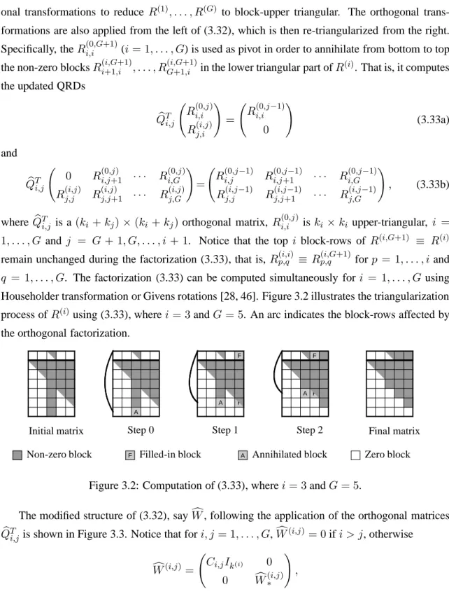
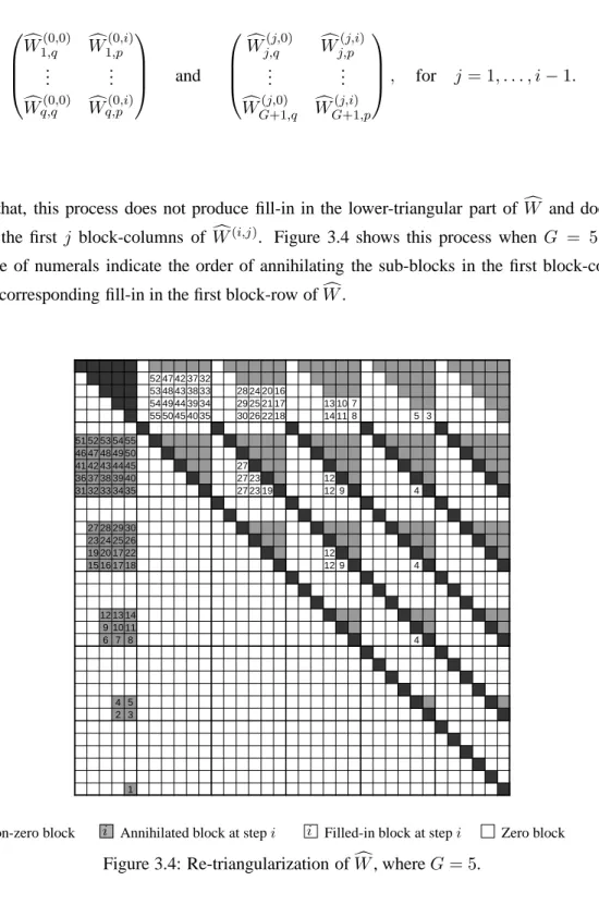
Chapter 3

Estimating seemingly unrelated

regression models with vector

autoregressive disturbances

Abstract:

The numerical solution of seemingly unrelated regression (SUR) models with vector autoregres-sive disturbances is considered. Initially an orthogonal transformation is applied to reduce the model to one with smaller dimensions. The transformed model is expressed as a reduced-size SUR model with stochastic constraints. The generalized QR decomposition is used as the main computational tool to solve this model. An iterative estimation algorithm is proposed when the variance-covariance matrix of the disturbances and the matrix of autoregressive coefficients are unknown. Strategies to compute the orthogonal factorizations of the non-dense structured matrices which arise in the estimation procedure are presented. Experimental results demonstrate the com-putational efficiency of the proposed algorithm.

1

This chapter is a reprint of the paper: P. Foschi, E.J. Kontoghiorghes. Estimating seemingly unrelated regression models with vector autoregressive disturbances. Journal of Economics Dynamics and Control, 2003 (In press).

(50)

3.1 Introduction

The seemingly unrelated regression (SUR) model is given by

yi =Xiβi+ui, i= 1,2, . . . , G, (3.1)

whereyi ∈RM is the endogenous vector,Xi ∈RM×ki is the exogenous matrix with full column

rank,βi ∈Rki are the coefficients andui ∈RM is the disturbance vector having zero mean. The

covariance matrix of ui and uj is given by σijIM (i, j = 1, . . . , G). In compact form the SUR

model can be written as

Vec(Y) = _⊕G_i₌₁XiVec({βi}G) + Vec(U), (3.2)

whereY = y1 · · · yG

,U = u1 · · · uG

,_⊕G_i₌₁Xi= diag(X1, . . . , XG),{βi}Gdenotes the set

of vectorsβ1, . . . , βGandVec(·)is the vector operator which stacks one column under the other of

its matrix or set of vectors argument. The disturbance termVec(U)_∼(0,Σ_⊗IM), i.e., it has zero

mean and dispersion matrixΣ_⊗IM, whereΣ = [σij]∈RG×Gis symmetric and positive definite

[3, 30, 69]. The subscriptGin the set operator{·}is dropped and⊕G

i=1is abbreviated to⊕i.

Often the SUR model has vector (VAR) or scalar (AR) autoregressive disturbances [26, 38, 43, 58, 65, 67, 79, 85]. In such cases the disturbance matrixU in (3.2) satisfies

U₋ZU AT =E (3.3a)

or, equivalently,

(IGM −A⊗Z) Vec(U) = Vec(E), (3.3b)

whereA_∈RG×Gis the matrix of the AR coefficients, theM_×M shift matrixZ is defined as

Z =           0 0 _{· · ·} 0 0 1 0 _{· · ·} 0 0 0 1 _{· · ·} 0 0 .. . ... . .. ... ... 0 0 _{· · ·} 1 0          

andE _∈RM×G. The dispersions ofVec(E)andVec(U)are given, respectively, byΣ_⊗IM and (IGM −A⊗Z)−1(Σ⊗IM) (IGM −A⊗Z)−T, (3.4)

(51)

3.1. INTRODUCTION 37 where₋T denotes the transpose of the inverse.

Now, premultiplying the SUR with VAR disturbances (hereafter SUR-VAR) model (3.2) by

(IGM −A⊗Z)it gives

Vec(Y ₋ZY AT) = (IG⊗X−A⊗ZX) (⊕iSi) Vec ({βi}) + Vec(E), (3.5a)

or the general linear model (GLM)

Vec(Ψ) =FVec (_{βi}) + Vec(E), (3.5b)

whereX _∈RM×Kd denotes the matrix comprising theKd distinct regressors of the SUR model and Si is aKd×ki selection matrix such that Xi = XSi (i = 1, . . . , G). The matricesΨand

F are defined by context. Notice that in the case where there are no common regressors, X and Si are given by X = X1 X2 · · · XG and Si = 0 Iki 0

, respectively. Furthermore, the matrixF in (3.5b) is full rather than block-diagonal as in the case of the conventional SUR model. The estimator of the SUR-VAR model (3.2) derives from computing the generalized least squares (GLS) estimator

Vec (_{βˆi}) = FT(Σ−1⊗IM)F−1FT Σ−1⊗IMVec(Ψ). (3.6)

In the case whereΣandAare unknown, an iterative procedure is used to derive the feasible GLS estimator. Initially,Vec (_{βˆi})is computed from (3.6) based on some initial estimates ofΣandA.

The residuals provide new estimates forΣandA, which are then used in (3.6) to derive a new GLS estimator. This procedure is repeated until convergence.

The existing methods for computing the GLS, or the feasible GLS, estimator of the SUR-VAR model solve the normal equation (3.6) explicitly by computing Kronecker products and inverses of matrices [43, 79]. This results in computationally expensive and numerically unstable estimation procedures [76]. The purpose of this work is to provide computationally efficient algorithms for computing the GLS estimator for the SUR-VAR model. These algorithms use non-literal Kronecker operations and for numerical stability use orthogonal factorizations [28].

In the next section the numerical solution to the SUR-VAR model is considered and an itera-tive algorithm to compute the feasible GLS estimator is proposed. Section 3.3 considers various strategies for computing the matrix factorizations arising in the estimation procedures of the model. Computational results are shown in section 3.4. Finally conclusions and future research are pre-sented.

(52)

3.2 Numerical solution of SUR-VAR models

Consider the QRD Kd _G _Kd _G ZX ZY X Y = K∗ K∗ M∗ Q∗A Q∗B Q∗C K∗ K∗       e R∗A RAe K ∗ 0 RBe K∗ 0 0 M∗ , (3.7) whereK∗ ₌_Kd₊_G_,_M∗ ₌_M ₋₂_K∗_,_R_e∗

AandRBe are upper-triangular defined by

e R∗A = Kd _G R∗ A YA∗ , RAe = Kd _G RA YA , RBe = Kd _G RB YB

and the orthogonal matrixQ∗_∈RM×M is partitioned as Q∗=Q∗

A Q∗B Q∗C

. (3.8)

Pre-multiplying (3.5) by the orthogonal matrix IG⊗Q∗A IG⊗Q∗B IG⊗Q∗C

_T gives     Vec(ΨA) Vec(YB) 0    =     IG⊗RA−A⊗R∗A IG⊗RB 0    (⊕iSi) Vec ({βi}) +     Vec(EA) Vec(EB) Vec(EC)    , (3.9) where ΨA =YA−YA∗A T _(3.10) and     Vec(EA) Vec(EB) Vec(EC)    ∼    0,     Σ_⊗IK∗ 0 0 0 Σ_⊗IK∗ 0 0 0 Σ_⊗IM∗        . (3.11)

From (3.11) it follows that (3.9), and consequently the SUR-VAR model, can be written as the SUR model