Eddie Gerba and Klemens Hauzenberger
Estimating US fiscal and monetary
interactions in a time varying VAR
Discussion paper
Original citation:
Gerba, Eddi and Hauzenberger, Klemens (2013) Estimating US fiscal and monetary interactions in a time varying VAR. School of Economics discussion paper , KDPE 1303. University of Kent, Canterbury, UK.
Originally available from the University of Kent
This version available at: http://eprints.lse.ac.uk/56393/ Available in LSE Research Online: April 2014
© 2013 The Authors
LSE has developed LSE Research Online so that users may access research output of the School. Copyright © and Moral Rights for the papers on this site are retained by the individual authors and/or other copyright owners. Users may download and/or print one copy of any article(s) in LSE Research Online to facilitate their private study or for non-commercial research. You may not engage in further distribution of the material or use it for any profit-making activities or any commercial gain. You may freely distribute the URL (http://eprints.lse.ac.uk) of the LSE Research Online website.
University of Kent
School of Economics Discussion Papers
Estimating US Fiscal and Monetary Interactions
in a Time Varying VAR
Eddie Gerba and Klemens Hauzenberger
March 2013
Estimating US Fiscal and Monetary Interactions in
a Time Varying VAR
Eddie Gerba and Klemens Hauzenberger
∗Abstract
We contribute to the growing empirical literature on monetary and fiscal in-teractions by applying a sign restriction identification scheme to a structural TVP-VAR in order to disentangle and evaluate the policy shocks and policy transmissions. This in turn allows us to study the Great Recession in a con-sistent fashion. Four facts stand out from our findings. We observe significant differences in the endogenous responses to shocks in particular between the Volcker period and the Great Recession, and find that monetary policy reacts more aggressively during Volcker chairmanship and fiscal policy during the Great Recession to stabilize the economy. Second, impulse responses confirm that there is a high degree of interactions between monetary and fiscal policies over time. Third, in the forecast error variance decomposition we find that while government revenues largely influence decisions on government spend-ing, government spending does not influence tax decisions. Fourth and final, our analysis of the fiscal transmission channel reveals that tax cuts, because of their crowding-in effects, are more effective in expanding output than govern-ment spending rises, since the tax multiplier is higher and more persistent. In light of the current recession and the zero lower bound of the interest rate, tax cuts can, by providing the right incentives to the private sector, result in high and very persistent growth in output if private agent expectations regarding the length and the financing structure of the fiscal expansion are delicately managed jointly by the two authorities.
JEL: C11, C32, E52, E61, E62, E63
Keywords: time varying parameter VAR, sign restrictions, Markov-Chain Monte Carlo, US economic structure, fiscal transmission channel
∗Gerba: School of Economics, University of Kent, Canterbury, CT2 7NZ, England
(email: [email protected]). Hauzenberger: Macroeconomic Analysis and Projection Divi-sion, Deutsche Bundesbank, Wilhelm-Epstein-Strasse 14, 60431 Frankfurt/Main (email: [email protected]). We would like to thank Jagjit Chadha for his advice and support, and Keisuke Casey Otsu for his useful comments. The views expressed in this paper are solely ours and should not be interpreted as reflecting the views of the Deutsche Bundesbank.
1
Introduction
Locating the appropriate degree of interaction between fiscal and monetary policy plays an important role in ensuring economic stability. This has been most evident during the Great Recession in the US, when on one hand, the Fed reduced the Federal Funds rate by more than 500 basis points from August 2007 and injected a vast amount of liquidity into the financial system through the three quantitative easings (the first announced in November 2008, the second in November 2010, and the third in September 2012). Worried additionally by the persistently high long-term yields, the Fed launched moreover two ‘Operation twists’ (first running between September 2011 and June 2012, and the second from July to December 2012) whereby the Fed exchange their shorter-dated liabilities for longer-term Treasuries in order to bring the prices of longer-term bonds up, and the yields down, while generating the opposite effect on the short-term bonds. In parallel, the US Congress passed two fiscal packages, the Economics Stimulus Act of 125 billion dollar in 2008, and the American Recovery and Reinvestment Act of 787 billion dollar in early 2009, and one fiscal reform, the Jump-Start Our Business Start-Ups Act in March 2012, a law intended to encourage funding of small businesses by easing a number of securities regulations. Their joint economic impact is, however, still unclear. The theoretical and empirical literature on fiscal-monetary interactions is equally inconclusive and points in multiple directions. It goes so far that there is no consensus to whether a (systematic or regular) coordination between fiscal and monetary policy ever existed in the US.
Against this background, our interest lies in examining in-depth the actual policy interactions over the past three decades (1979-2012). We allow for changes in the US economic structure, and jointly study the effectiveness of monetary and fiscal policy in stabilizing the economy. Further, we will examine the fiscal transmission mechanism and monetary pass-through over time and provide empirical evidence on the structural shocks that have been most important in explaining the fluctuations of the US economy over this period.
There is a richer theoretical literature on fiscal-monetary interactions compared to the empirical.1That is an outcome that has evolved from the difficulty of
com-1They find that it is very important to jointly study the fiscal and monetary policy in order to determine the equilibrium. Chadha and Nolan (2007) find that Taylor-like monetary and fiscal rules are a good representation of US and UK stabilization policies. Neglecting the role of automatic stabilizers in designing the optimal policies has immediate effects for the optimal monetary policy. So, for instance, a passive fiscal policy requires a large long-run response of the policy rate to
paring theoretical and empirical results. When appropriate care is taken for the diverse complications inherent in macroeconomic time series, such as unit roots, and in the case of policy decisions, real time versus revised data, then results from standard theoretical and empirical models strongly diverge (Reade and Stehn, 2008, and Juselius, 2007). As a consequence, the empirical models have departed from their theoretical counterparts.
Several interesting insights have emerged from the empirical fiscal-monetary models. Fragetta and Kirsanova (2007) model policy interactions in the UK, Sweden and the US. Using Leeper’s (1991) definition of leader and follower they investigate whether one or the other authority has acted as a leader. They find no evidence for dominance in the US, and suggest that the two authorities ignore each other. On the other end, Muscatelli et al. (2004), using generalized methods of moments, estimate a forward-looking new-Keynesian model for the US. They find that depending on the shocks considered, the nature of fiscal-monetary interactions has been different. For business cycle shocks, monetary and fiscal policies act as compliments, meaning that when monetary policy is tightened, so is fiscal policy. However, for a monetary shock, a tighter monetary policy results in a relaxed fiscal policy, hence acting as substitutes. Reade and Stehn (2008) also find evidence for policy interactions in the US, since both policies are countercyclical, and each of them takes into account the actions of the other. Conversely, Melitz (2002) finds that monetary and fiscal policies move in opposite directions, thus behave as substitutes. On the economic effects of the two policies, Melitz (2002) and Muscatelli et al. (2004) find that spend-ing responds in a destabilizspend-ing manner to current output, while taxes behave in a stabilizing fashion.2For monetary policy, Muscatelli et al. (2004) detect a
stabiliz-inflation for the previous optimum to be reached (Chadha and Nolan (2007), Annicchiarico et al (2012)). Davig and Leeper (2010) estimate Markov-switching policy rules for the US and find that the monetary and fiscal policy fluctuate between active and passive behavior. In a New-Keynesian model, this results in positive spending multipliers, but the intensity of the multiplier depends on the degree of crowding out in private consumption and investment that the policy causes. Moreover, Annicchiarico et al (2012) argue that the fiscal expansions tend to generate an intertemporal trade-off. The positive fiscal shocks are expansionary in the short-run, but depending on the monetary policy rule pursued, are likely to generate persistent adverse effects in the medium-run. Baxter and King (1993), and Davig and Leeper (2010) find that the negative effects of fiscal policy result from the higher tax burden in the future. Finally, Gali and Monacelli (2008) show that in a currency union with country-specific shocks and nominal rigidities, inflation should be stabilized at the union level, while the countercyclical fiscal policy should be country-specific when the latter seek to limit the size of the domestic output gap and inflation differentials resulting from idiosyncratic shocks.
2Muscatelli et al. (2004) find, however, that spending responds in a stabilizing manner to lagged output.
ing role of the interest rate relative to output, and Reade and Stehn (2008) show that monetary policy has a stronger impact on economic activity compared to fiscal policy.
In short, the empirical results are inconclusive, and depend strongly on the methodology used. Nevertheless, the majority of them point at least toward an im-plicit coordination between monetary and fiscal authorities, and indicate a greater effectiveness of monetary policy in dampening output volatility.
We use the recently established structural time varying parameter VAR (hence-forth TVP-VAR) to examine US policies between 1979:I-2012:II. The structural TVP-VAR was put forward by Cogley and Sargent (2005) and Primiceri (2005) to establish and examine the different monetary policy regimes that the US has under-gone since the post-war period. While they observe some deviation in the impulse responses during the oil-shocks and early Volcker period, for the remaining sample, they find insignificant time-variation. Moreover, they note that most of the variation is attributed to the variance of the residuals, and not to the coefficients. Separately, Kirchner et al. (2010) and Pereira and Lopes (2010) have used a TVP-VAR to ex-amine the effect of fiscal policy shocks. While the former has employed a recursive assumption to identify spending shocks, the latter use the method of Blanchard and Perotti (2002) to identify tax and spending shocks.3More recently, Hauzenberger (2012) has performed a similar analysis for a fiscal TVP-VAR with a special focus on debt dynamics but which does not include the monetary side.
The study closest to ours is Rossi and Zubairy (2011).4They jointly consider
mon-etary and fiscal shocks in their analysis of the US economy, and find that conditioning monetary policy and fiscal policy on each other is crucial for producing unbiased estimates of the business cycle drivers. Additionally, by means of variance decom-positions, they find that monetary policy shocks are most important for explaining business cycle fluctuations in output, consumption and hours, while fiscal policy shocks are most important for explaining cyclical volatilities over the medium-term. Nevertheless their study was performed using a fixed-coefficient structural VAR and so the contribution of each shock is invariant during that sample period. In the same manner, the fiscal transmission channel is not allowed to alter with changing
3See also Fatas and Mihov (2001) for recursive assumptions.
4Mountford and Uhlig (2009) falls to a certain extent into this category. They identify both monetary and fiscal shocks, but concentrate their analysis on the effects of fiscal policy and not the interaction between the two policies. Monetary policy is identified in order to isolate its effects from fiscal policy.
economic conditions. Our TVP-VAR will correct for this omission by allowing the shocks and the fiscal transmission to vary over time.
Our empirical approach is based on a five variable version of the Bayesian TVP-VAR technique with stochastic volatility. The variables we include are output, gov-ernment spending, net taxes, a short-term interest rate and inflation. We identify four shocks—business cycle, monetary policy, spending, and taxes—through theo-retically robust sign restrictions. There is a fifth shock in this model (a residual shock), but because the shock is activated by innovations in one of the other model variables, it is not identified and therefore does not have a structural interpretation. Moreover, the sign restrictions are a partial identification method and there is there-fore no necessity to identify as many fundamental shocks as variables in our model (see, e.g., Uhlig, 2005). Further, identifying a business cycle shock jointly with the other shocks is crucial to separate automatic effects of output fluctuations from dis-cretionary policy measures (Mountford and Uhlig, 2009). In the context of policy interactions, the sign restrictions framework does not oblige us to impose timing assumptions regarding the fiscal-monetary interaction, since the interactions can be contemporaneous or lagged, thus implying more adequate empirical results. Lastly, allowing the volatility of errors to vary over time is becoming increasingly impor-tant in macroeconomics, not only because the volatilities of many macroeconomic variables have changed over time (e.g. going from the 1970’s to the Great Modera-tion in mid-80’s.), but also because many issues of macroeconomic policy hinge on error variances of, amongst other, price and output levels. For these reasons, we wish to capture these volatility variations in our model, and study the responses of monetary and fiscal policies to these shifts in the economy.
The paper makes four principal contributions. First, we observe significant time variation in the model parameters (and volatilities of residuals) between 1979 and 2012. All our results confirm that there are three regimes in the US economy: the Volcker chairmanship (1979-84), the Great Moderation (1985-2007), and the Great Recession (2008-12). More specifically, we observe significant differences in the en-dogenous responses to shocks in particular between the Volcker period and the Great Recession, and find that monetary policy reacts more aggressively during Volcker chairmanship and fiscal policy during the Great Recession to stabilize the economy. Second, impulse responses show that there is a high degree of interactions between monetary and fiscal policies over time. Whereas for a tax shock, the policies act as substitutes, we note significant time variation for the other shocks. On one hand,
the two policies behave as substitutes for both the monetary policy and govern-ment spending shocks during the Volcker era, while on the other, they behave as compliments during the Great Recession. Moreover, both the monetary and (net) fiscal policy has a stabilizing effect on output, albeit government spending behaves in a destabilizing fashion. Third, decomposition of forecast error variance of gov-ernment spending shows that spending itself is largely acyclical, indicating strong inertias and path-dependencies in spending decisions. In addition, we find that while government revenues largely influence decisions on spending, spending does not influence tax decisions. Along the same lines, we observe a significant degree of coordination between monetary and fiscal authorities in the decomposition exercise where both authorities take into account the decisions of the other. Fourth and final, our analysis of the fiscal transmission channel reveals two things. Tax cuts, because of their crowding-in effects, are more efficient in expanding the economy than government spending rises, since the tax multiplier is higher and more persis-tent, in particular during the Volcker regime. The second thing we note is that fiscal shocks are more quickly transmitted onto prices than the monetary policy shock. This suggests there might be frictions in the US monetary transmission channel, such as financial market frictions (banking, credit, leverage) that cause a delayed response of prices to monetary policy shocks.
The remainder of the paper is outlined in the following way. Section 3.2 de-scribes the econometric framework, including data, the identification scheme, the model specification, and the Bayesian technique used (further details on Bayesian inference including the sampling algorithm and the convergence diagnostics of the Markov chain are explained in Appendix I). We go on by discussing our first results from the impulse responses in section 3.3, where we also try to identify different fiscal-monetary regimes in the US. In addition, we identify and analyze the fis-cal multipliers in the same section, and compare our findings to a fixed coefficient structural Bayesian VAR. In section 3.4, we establish the importance of fiscal and monetary shocks as drivers of output and the other variables in our model. Section 3.5 concludes.
2
Econometric Methodology
The method we use is a structural time varying vector autoregressive model (TVP-VAR) with sign restrictions estimated on quarterly US data from 1979:I to 2012:II.
We allow for variation over time in the estimated coefficients of the model and in the variance-covariance matrix of the residuals. This is a strong advantage over fixed-parameter VARs as it allows us to capture any gradual structural shifts that might occur in the economy att= 1, . . . , T. Our results are derived from analyzing (structural) impulse response functions and forecast error variance decompositions. The flexibility of a TVP-VAR does not come without costs. The computational burden increases rapidly with the number of endogenous variables, lags and the set of identifying restrictions. To keep the amount of parameters and restrictions manageable, we will restrict ourselves to five variables and two lags.5Moreover, we identify the shocks randomly distributed only once within three specific regimes. The first regime corresponds to the Volcker chairmanship (1979-1984); the other two somewhat loosely to the Great Moderation (1985-2006) and Great Recession (2007-2012). Although focusing on a few regimes instead of everyt slightly restricts the flexibility of the time varying approach but, on the other hand, such a focus can be thought as a more elaborate subsample strategy. Primiceri (2005) has implicitly taken and defended a similar route.
2.1
Model Specification
Thek-vector of quarterly variables {yt}Tt=1 includes government spending, net taxes,
output, inflation and a short-term interest rate in that order. We assume yt =
(yg,t, yt,t, yx,t, yπ,t, yi,t)
0
evolves according to the TVP-VAR(p) process,
yt=Ct+B1,tyt−1+· · ·+Bp,tyt−p+ut, (1)
in whichCt is a k×1 vector of time varying intercepts,Bi,t (i= 1, . . . , p) is a k×k
matrix of time varying coefficients andut are possibly heteroscedastic reduced-form
residuals with variance-covariance matrix Ωt. Iterating on (1) yields the
correspond-ing infinite movcorrespond-ing average representation, i.e.
yt =µt+
∞
X
h=0
Θh,tut−h. (2)
5Primiceri (2005), and Cogley and Sargent (2005) employ a 3-variable monetary TVP-VAR. Kirchner et al. (2010), Pereira and Lopes (2011), and Hauzenberger(2012) use a 4-variable fiscal TVP-VAR. All these papers use two lags.
Θ0,t =Ik, or a k dimensional identity matrix, µt =
P∞
h=0Θh,tCt and Θh,t =JB˜thJ
0
in which ˜Btis the corresponding TVP-VAR(1) companion form of the TVP-VAR(p)
in (1) andJ denotes a selector matrix:6 ˜ Bt= " Bt Ik(p−1) : 0k(p−1)×k # and J = Ik : 0k×k(p−1) . (3)
The parameters Θh,t for h= 1, . . . , H represent the reduced-form impulse response
functions. To transform these responses into ones with a structural interpretation we proceed in two steps. First, we decompose the reduced-form variance matrix Ωt
in a standard triangular fashion and then, in a second step, we identify the structural shocks through sign and other restrictions on the impulse responses. Specifically,
ut=A−t1ΣtGtεt (4)
in which εt are the normalized structural shocks (i.e. εt ∼ N(0, Ik)), At is lower
triangular with ones on the main diagonal;
At= 1 0 0 0 a21,t 1 0 0 .. . . .. . .. ... an1,t · · · ann−1,t 1, (5)
Σt is a diagonal matrix with entries σi,t (i = 1, . . . , k), or a matrix of uncorrelated
variances; Σt= σ1,t 0 0 0 0 σ2,t 0 0 .. . . .. ... ... 0 · · · 0 σk,t, (6)
andGtis an orthonormal rotation matrix. Given the properties ofGt andεt we can
write the decomposition of the reduced-form variance-covariance matrix as
Ωt=A−t1ΣtΣ
0
tA
−10
t . (7)
6We will see in just a short while thatI
This is the first step in our transformation into structural impulse responses. There-fore, combining 4 with the reduced-form impulse response function on the right-hand side of 2, the structural impulse responses follow then from:
Φt= Θ00,t :· · ·: Θ
0
H,t
0
A−t1ΣtGt, (8)
in which we rotate the orthonormal matrix Gt until Φt satisfies all the imposed
restrictions, and the forecast error variance decomposition of yt can be extracted
from the diagonal elements of
Ω(y)h,t = H
X
h=0
Θh,tΩtΘ0h,t. (9)
This is the second step. We have now identified the complete structural impulse responses, including the forecast error variance decomposition. Let us continue by re-writing the TVP-VAR (p) model 1.
For the estimation it will be practical to collect the slope coefficientsBt= (B1,t:
· · ·:Bp,t) in a k×kp matrix and to transform it together with the constant into a
k(kp+ 1) vector of VAR coefficients by stacking the columns, i.e. βt= vec (Bt:Ct).
The model in (1) can now be rewritten as
yt=Xt0βt+At−1ΣtGtεt, (10) Xt0 = y0t−1 :· · ·:y 0 t−p : 1 ⊗Ik,
in which the operator⊗ denotes the Kronecker product. Like the VAR coefficients, we bring the non zero and one elements of the covariancesAtand volatilities Σt into
vector form: αt = (α21,t, α31,t, α32,t· · · , αk1,t,· · · , αkk−1,t)0 and σt = (σ1,t,· · · , σk,t)0
where the corresponding dimensions arek(k−1)/2 andk. This way of decomposing the variance-covariance matrix in 10 is not unique to the TVP-VAR literature, but is also widely applied in the literature considering the problem of efficiently estimating covariance matrices.7
The vectors αt, βt, and σt summarize all the time varying parameters of the
model.8We have in effect transformed the TVAP-VAR(p) expression 1 into 10. In 7See Pourahamadi (2000), or Smith and Kohn (2002).
8In Cogley (2003), and Cogley and Sargent (2005), α is time invariant, meaning that an innovation in the i-th variable has a time invariant effect on the j-th variable. However, our purpose is to model time-variant simultaneous interactions of equations, which means thatαmust be allowed to vary over time.
effect, the new strategy is to model the coefficient processes in 10. As in Primiceri (2005) we let the coefficients αt and βt evolve as random walks and the standard
deviationσt follows a geometric random walk:
αt=αt−1+ζt (11)
βt=βt−1+νt, (12)
logσt= logσt−1+ηt. (13)
The specification for σt falls into the class of models known as stochastic volatility.
While in infinite samples a random walk hits an upper or lower bound for sure, the use of finite samples makes it possible to maintain the random walk assumption. A great advantage as we do not have to estimate additional parameters, although, in principle, we could extend (11), (12) and (13) to represent more general autoregres-sive processes.9
The innovations εt, ζt, νt, and ηt are mutually uncorrelated Gaussian white
noises with zero mean and variances defined by the identity matrix Ik and the
hyperparameters Q, S and W.10Summarized in the variance-covariance matrix V
we have: V = Var εt νt ζt ηt = Ik 0 0 0 0 Q 0 0 0 0 S 0 0 0 0 W , S = S1 0 · · · 0 0 S2 . .. ... .. . . .. ... ... 0 · · · 0 Sk−1 , (14)
S1 = Var([∆α21,t]0) and Si−1 = Var([∆αi1,t,· · · ,∆αii−1,t]0) for all i = 3, . . . , k. All
matrices here, besides the identity matrix Ik, are positive definite. The rather
specific assumptions on the structure of V and S are standard in the literature (see, e.g., Primiceri, 2005, and Canova and Gambetti, 2009) and are not essential to keep the estimation feasible. The structure of V and S offers, however, numerous advantages: most important for our purpose is that the block diagonality ofS with 9Primiceri (2005) does extend the framework as a robustness check, and allows the coefficients and log standard errors to follow a more general AR process (varying the AR coefficients between 0.5 and 0.95). He does, however, not find any significant differences for the model performance compared to the random walk hypothesis. The only minor change is that the model captures, apart from the permanent, many temporary variations in parameters. The temporary changes are, nevertheless, irrelevant for the overall analysis.
10The priors for the model coefficients in 10 and hyperparameters are outlined and explained in Appendix II.
blocks corresponding to parameters in separate equations of the TVP-VAR enables us to model [α21,t], [α31,t, α32,t] , . . . , [αk1,t,· · · , αkk−1,t] in linear state space form.
The advantage of linearity will become clear when we lay out the Bayesian estimation strategy for our model. Also, assuming all off-diagonal elements to be zero does not further exaggerate the curse-of-dimensionality problem (i.e. a very large number of parameters) inherent in all time varying parameter models.
2.2
Identification
We use sign restrictions, summarized in Table A.1, to identify jointly four orthogonal shocks: a business cycle shock which increases output and taxes; a monetary policy shock which increases the interest rate and decreases inflation and output; a spend-ing shock which increases spendspend-ing and output; and a tax shock which increases taxes and decreases output. In addition, there is a residual shock in this model.11 However, because it is not identified, it does not have a structural interpretation, and therefore we do not report it. Moreover, sign restrictions are a partial identification method and there is therefore no necessity to identify as many fundamental shocks as variables in our model (see, e.g., Uhlig, 2005). All restrictions must hold for one quarter, except for the responses of the variables which are directly associated to the shock (e.g. tax shock on taxes), they must hold for two quarters. Having some-what longer restrictions here rules out transitory effects. The signs of the restricted responses are relatively uncontroversial and consistent with most dynamic general equilibrium models and Keynesian aggregate supply and demand diagrams.12
Of course, such a strong view on the sign of the responses discards, at least on impact, more controversial phenomena such as expansionary fiscal contractions (see, e.g., Giavazzi et al., 2000) or the price puzzle. With our strong view we avoid however some issues often criticized in the structural VAR literature, for example the missing link between theory and a simple Choleski decomposition (i.e. a causal ordering of the variables) or the weak information provided by sign restrictions if one takes a too agnostic view on the identification of shocks (see, e.g., Canova and Pina, 2005, and Canova and Paustian, 2011). Being too agnostic may have especially severe consequences if the relative variance of the shock of interest delivers a weak
11The residual shock can be viewed as innovation to inflation in u t.
12Canova and Pappa (2007), Mountford and Uhlig (2009), and Pappa (2009) apply a similar identification scheme through sign restrictions to study the effects of fiscal policy, and Chadha et al (2010) apply a similar scheme to a monetary policy framework.
signal. The usual suspect here is the monetary policy shock. So the relatively large number of theory driven restrictions and our rich shock structure should a-priori lead to a good performance and reliability of our approach.
Although it is not of our primary interest, identifying a business cycle shock is crucial to adequately track the source behind the fiscal shocks, especially on the tax side (see, e.g., Blanchard and Perotti, 2002, and Mountford and Uhlig, 2009). In this way we can disentangle whether a change in taxes comes from fluctuations in output or a tax shock. Just as a remark, we do not differentiate between a demand driven or supply driven business cycle shock; the results will, however, provide us with an indication of the relevant driver in a particular regime.
In addition to restricting the signs we also impose magnitude restrictions. First, we narrow down the elasticity of taxes to output in the matrix of contemporaneous effects G0tΣ−t1At. Most papers in the tradition of Blanchard and Perotti (2002)
predetermine this elasticity, the one which essential separates tax and business cycle shocks, at values somewhere around (minus) 2. Hauzenberger (2012) estimates time varying elasticities over the last 45 years and finds values larger than zero but lower than 3. Accordingly, we limit the respective coefficient in the G0tΣ−t1At matrix to
that range and in the same way we restrict the spending and tax multipliers to be lower than 3 on impact. Such an upper restriction on the impact multiplier is relatively liberal and captures most of the values found in the literature (e.g., Ramey, 2011, Romer and Romer, 2012, and Favero and Giavazzi, 2012). Kilian and Murphy (2012) show how imposing plausible bounds effectively reduces the number of admissible but empirically implausible models. Second, in certain cases it is not possible to fully disentangle the four shocks by the restrictions in Table A.1. When the candidate response for a spending shock implies an increase in taxes, it could also represent a business cycle shock. Rather than discarding, and essentially imposing a negative sign on the response of taxes to a spending shock, we disentangle the two shocks through a relative magnitude restriction: a business cycle shock that increases output by one-dollar must have a larger effect on taxes in absolute terms than a one-dollar spending shock. The relative magnitude restriction must hold for two quarters.13This procedure further helps in reducing the number of implausible models (see, e.g., Dungy and Fry, 2009).
13Two quarters is a reasonable assumption since cyclical movements have a longer lasting impact on taxes than spending. However, the results do not significantly change if the relative magnitude restriction is applied only for one quarter. In any case, this assumption is much less restrictive than the negative tax response restriction.
We have started the project with the ambitious goal of identifying jointly the four shocks in every periodt. As it turned out, such a goal is computationally too demanding and we therefore opted for a different strategy, identifying the shocks only once within the three specific regimes of the Volcker chairmanship (1979-1984), the Great Moderation (1985-2006) and the Great Recession (2007-2012).14Formally,
defineS as the set of sign and magnitude restrictions, and letG(tr) be one orthonor-mal rotation matrix in (8).15Then, to find one representative impulse response for
the Volcker Chairmanship,
ΦV = Θ00,t :· · ·: Θ 0 H,t 0 A−t1ΣtG (r) t , (15)
we randomly pick a quartert from TV, TV + 1, . . . , TM −1 and rotate G
(r)
t overr =
1,2, . . . , Runtil there is oner such thatS ⊂ΦV; and in the same way we search for
ΦM and ΦG in the Great Moderation and Great Recession witht∈(TM, . . . , TR−1)
and t∈ (TR, . . . , T). The specific dates defining the three regimes are TV ≡1979:I,
TM ≡ 1985:I and TR ≡ 2007:I. If we fail to find an admissible impulse response
within the maximum numberR of allowed rotations, we pick a different t and start our search again.
As a robustness check of our identification procedure we also run a recursive scheme. It will be a pseudo recursive identification, to be precise, because we keep rotating the two-by-two block of taxes and output to separate the tax and business cycle shocks. Unlike spending and monetary policy shocks, which can be identified by ordering spending first and the short-term interest rate last (see, e.g., Perotti, 2007, and Christiano et al., 2005) the other two shocks cannot be identified by a simple causal ordering. Therefore, to have a better comparison with our main identification procedure we keep the sign restrictions on the tax-output block.
2.3
Estimation
We estimate our TVP-VAR using Bayesian methods on quarterly data from 1979:I to 2012:II for our five variables: government spending, net taxes, output, the in-flation rate and a short-term interest rate. To keep our results comparable with 14Since our sample includes over 130 quarters, identifying all sign restrictions in each quarter is computationally very demanding and results in many unstable draws. We therefore opt for the alternative strategy outlined below, which moreover is standard in the TVP-VAR literature.
15G(r)
t comes from a QR decomposition of a k×k standard normal matrix with the upper triangular part normalized to be positive.
Blanchard and Perotti (2002) and other studies in their tradition, we define the fiscal variables in the same way: government spending includes both government consumption expenditures and gross investment, and net taxes are the current re-ceipts less net transfers and net interest paid. Note that these are not expressed as ratios to GDP, but directly in levels (in order to facilitate the interpretation of these variables to the various shocks). On the nominal side we measure inflation as the quarterly change of the output deflator and use the 3-month T-bill rate as our short-term interest variable; both are expressed in percent per quarter.16The three variables on the real side of the economy enter the TVP-VAR as the logarithm of their real, per-capita values.17The TVP-VAR is estimated in levels.18
Since we do not have a closed form solution for the posterior distribution of the structural parameters we use a Markov chain Monte Carlo (MCMC) algorithm for the numerical evaluation. Taking the Bayesian route together with somewhat informative priors effectively deals with the large dimensionality of the TVP-VAR compared to maximum likelihood techniques where it is hard to rule out peaks in the likelihood in uninteresting regions of the parameter space. Estimation further exploits the fact that it is typically easier to draw from a lower dimensional distribu-tion, conditional on a set of parameters. Specifically, conditional sampling requires to treat the VAR coefficients βt, the covariances αt and the volatilities σt as
sepa-rate blocks in a Gibbs sampler.19 Appendix B has a detailed exposition of our prior choice and the sampling strategy.
The Gibbs sampler does not ensure that every single βt from a draw of the
sequence {βt}Tt=1 leads to a stable VAR representation. Cogley and Sargent (2005)
discard a draw as soon as they find aβtwith eigenvalues larger than one in modulus.
Such a strict rule may not be practical here for two reasons: one is policy related 16Using the Federal Funds rate instead of the T-bill does not change the results.
17The data sources are the National Income and Product Accounts (NIPA) from the Bureau of Economic Analysis (BEA) and the Federal Reserve Economic Data (FRED). Specifically, NIPA tables 1.1.4 (line 1), 1.1.5 (lines 1 and 21), 3.1 (lines 1, 9, 11, 15 and 22), 7.1 (line 18), and FRED series TB3MS for the 3-month T-bill rate. All variables were downloaded on September 1, 2012.
18Mixing the I(0) and I(1) data for the Bayesian TVP-VAR estimation is not unusual in the literature and has been applied by, amongst others, Kirchner et al (2010), and Nakajima (2011). Another example is Christian et al (2005) who estimate their New-Keynesian model using Bayesian methods and a mix of I(0) and I(1) data. We deal with it by imposing a mild stability condition on the first differences. Specifically, we check the roots of the associated VECM polynomial of the VAR and discard every draw that has more than k = 4 roots in or on the unit circle. See Hauzenberger (2012) for more details on this transformation of the level TVP-VAR(p) in 1 and for checking the roots.
19Gelman et al. (1995, Chap. 11) show that the stationary distribution of the Markov Chain generated by the Gibbs sampler is the joint distribution one is looking for.
and the other one is of statistical nature. Unlike monetary policy the objective of fiscal policy does not necessarily lie in stabilization, and the use of spending, taxes and output in levels basically rules out stability. It is therefore more practical to impose a relatively weak condition on a quasi differenced version of the model in which we transform the autoregressive coefficients in the spending, tax and output equations to represent a specification in first differences.20
After a burn-in period of 50,000 iterations we start saving every third draw from the joint posterior distribution until a total of 20,000. The “thinning” helps to break the autocorrelation of successive draws; Appendix B.3 provides satisfactory conver-gence diagnostics of the MCMC chains. All of the 20,000 saved draws must satisfy the sign, magnitude and stability restrictions. Specifically, for each of the 20,000 draws we randomly pick a quarter from the Volcker period, the Great Moderation and the Great Recession and generate the impulse responses from (15). As a result, we get three distributions of impulse responses that are representative for the effects, interactions and the transmission of fiscal and monetary policy in our three episodes. In the discussion we will focus on the median as a summary measure. The median is not uncontroversial: Fry and Pagan (2007) criticize the lost orthogonality prop-erty of the shocks when the summary measure mixes different draws of admissible models. Their remedy to restore orthogonality suggests to use the single model that comes closest to the median. Canova and Paustian (2011) dig a little deeper into the issue and find the median to be an acceptable summary measure, performing reasonably well compared to Fry and Pagan’s (2007) close-to-median rule.
3
Fiscal and Monetary Interactions
We organize the discussion of the results in the following way. Section 3.1 discusses the time variant volatility pattern of the estimated model coefficients. We continue by analyzing the endogenous responses to business cycle, government spending, tax and monetary policy shocks. A business cycle shock is defined as a shock that jointly moves output and taxes in the same direction. This is an important assumption because when output and taxes move in the same direction, we essentially assume that this must be due to some improvement (deterioration) in the business cycle generating the increase (fall) in taxes, not the other way around. Moreover, the 20See Hauzenberger (2012) for more details about imposing a weak stability rule on variables in levels with an obvious trend.
effect of the business cycle shock on taxes (in absolute terms) must be larger than the effect of a spending shock for two consecutive quarters following the shock. Identifying a business cycle shock is crucial to adequately track the source behind the fiscal shocks, especially on the tax side (see, e.g., Blanchard and Perotti, 2002, and Mountford and Uhlig, 2009). In this way we can differentiate between automatic stabilizers and active policy decisions.21In addition, there is a fifth shock in this
model, a residual shock. However, because it is not identified, it does not have a structural interpretation, and therefore we do not report it. Moreover, the sign restrictions are a partial identification method and there is therefore no necessity to identify as many fundamental shocks as variables in our model (see, e.g., Uhlig, 2005).
Our main interest is in detecting possible structural shifts in the economy, as well as shifts in the application of both monetary and fiscal policy. In addition, we hope to find sufficient evidence to determine when and whether the three policies (monetary, spending, and tax) have stabilizing or destabilizing effects on output. We compare our findings with the key results in the literature.
However, before we begin the discussion, we would also like to introduce some key concepts that we will be making use of throughout the subsequent sections. The first one refers to interaction and coordination of the two policies. Following the large literature on policy interactions, if the two policies exhibit a positive or neg-ative correlation (or a common cyclical pattern) implying that one policy responds strategically to the actions of the other (in whatever direction), we say that the two policies interact, or coordinate their responses. Going one level deeper and following Muscatelli et al (2004), if the interaction has a positive correlation, we define the two policies as being compliments. In contrast, if the two policies have a negative correlation, then the two policies act as substitutes. Finally, the last level of policy analysis regards the responses of the two policies to innovations in output, as in Melitz (2002) and Muscatelli et al (2004). If the interest rate rises after a business cycle shock, we say that the monetary policy acts in a stabilizing fashion. Likewise, if taxes rise, or government spending falls following the same business cycle shock, we equally say that the fiscal policy acts to stabilize output. Since we superimpose via our identification scheme that taxes will always rise following a positive business cycle shock, the final outcome on the fiscal side will therefore depend on the sign 21While we only consider the movements in total government revenues, and not in the marginal tax rate textitper se, Baxter and King (1993) show that since the end of the war (1944-45), the two have moved tightly together and thus can be viewed as the same thing.
and the magnitude of responses of government spending.
3.1
Time Variant Volatility Patterns
Looking at Figure II.1, we can identify at least two periods of exceptionally high volatility in the residuals of the TVP-VAR equations. The first one is at the be-ginning of our sample period (1979-1984) which falls under the early Volcker period (in line with the findings of Primiceri, 2005), when the interest rate and inflation experienced their highest peak, as well as output and spending.22The second period is during the Great Recession (2007-2012), when the volatility of taxes increased, and that of output and spending to a certain extent. In the two decades preceding it, the volatility of the two variables was maintained at a constant level. We should therefore expect to see more volatility in impulse responses during those two peri-ods compared to the Great Moderation (1985-2006). This is interpreted as a first indication that there are these three regimes in our data.
3.2
Impulse Response Analysis
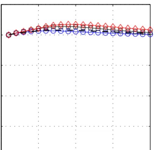
The impulse responses are reported for the three distinct periods in Figures II.2 to II.5. The blue line with circles corresponds to the median response during the Vol-cker era (1979-1984). The second represents the median response during the Great Moderation (1985-2006), while the third is the median impulse response during the Great Recession (2007-2012). We initially performed a fully flexible and time-variant scheme, allowing the shocks to be identified in every quarter, but detected that most time-variation occurred between the three regimes. Since minimal variation was ob-served within those three regimes, and in order to keep our discussions focused, we follow the approach by Primiceri (2005) and Kirchner et al. (2010), and in the same figure report the representative (i.e. median) response for each regime.
The reader will notice that some impulse responses are reported in terms of “percent or percentage deviations from trend”, while others are reported in terms of “dollar deviations from trend”. The responses of output, spending and taxes to a business cycle, spending and tax shock are therefore reported in terms of (non-cumulative) multipliers (see Blanchard and Perotti, 2002, and Kirchner et al., 2010). 22Since output and spending are specified in levels in the estimations, we observe the increase in volatility as an increase in level. Another possibility would have been to express the two variables in quarterly growth rates, just as the interest rate and inflation, whereby we would observe a similar peak in the former like we observe in the latter two.
In other words, we convert the initial estimates of the variables we use in log-levels output, spending and taxes from elasticities into derivatives by multiplying it with the prevailing ratio of the responding and shocked variables. For the spending mul-tiplier we can write this conversion as (the same conversion applies to the remaining two variables): ∆Yt+h ∆Gt+h = Yt Gt ∂logYt+h ∂logGt+h , h= 0,1, ..., H (16) in whichYt and Gt are the levels of output and spending,H defines the impulse
response horizon, and the log-derivatives follow from (8). The prevailing ratio (Yt
Gt in this case) is independently calculated for each regime by randomly selecting a quarter within a regime (Volcker Chairmanship, Great moderation, and Great Recession separately). Once a quarter in each regime which satisfies all the sign restrictions has been located, the ratio is calculated based on the values obtained in that quarter. Thus, the ratio is also time varying. The size of all shocks are normalized and represent, depending on the units of the shocked and the response variable, either a one dollar, percent or percentage point innovation.
The first thing to note is that there is significant time variation in the impulse responses. The magnitudes in the responses differ considerably between the regimes. Moreover, for government spending and monetary policy shocks, we observe a qual-itative difference in responses besides the quantqual-itative. This confirms our selection of the three regimes (or economic structures) in our sample. This is in stark con-trast to the findings of Cogley and Sargent (2005), Primiceri (2005), and Koop and Korobilis (2009) who find the majority of the time variation in the variance of the residuals, but not in the TVP-VAR coefficients.23We believe that the disparity in our results reflect the fact that we have included fiscal variables and shocks in our model, thereby studying much richer dynamics. This explanation is supported by the findings of Rossi and Zubairy (2011) described in the introduction. Also, Kirchner et al. (2010) and Pereira and Lopes (2010) find significantly higher time variation in the impulse responses in their fiscal TVP-VAR compared to a monetary one.
Second, we observe minor differences between our sign-restriction approach and the recursive. In most cases, there are only minor differences in magnitudes of the responses, but qualitatively they are the same. The only exception is the monetary policy shock, where we observe some differences between the two methods. There 23More recently, Kim and Yamamoto (2012) have found statistically significant evidence of time varying coefficients in a simple monetary model.
are two reasons for that. The first is related to the weak impact of the monetary policy shock. The literature on sign restrictions has found that without imposing the restrictions on some of the variables in the model, the impact of the shock is marginal. Therefore in order to generate the impact in line with the theoretical literature, you need to impose plenty of sign restrictions on the model (Canova and Paustian, 2011). In our case, we impose restrictions on three variables: output, inflation, and the interest rate. This is of course absent in the recursive approach. The second is related to the fact that in the recursive approach, the interest rate is ordered last in the model, resulting in a lag on the impact of the monetary policy shock on the remaining variables. This is, however, inconsistent with the theoretical literature, which finds an immediate impact of monetary policy on the economy. In this sense, our framework is more appropriate since we observe contemporaneous effects of the monetary policy.
To summarize, our method comparison shows that our identification scheme is consistent and robust. For most shocks, we only observe some minor differences in the magnitudes of the impulse responses, which, taking into account that our shocks are well identified, means that our results are reliable. Further, the advantages derived from applying sign restrictions for a monetary policy shock indicate that our method is preferred to the recursive. Let us now have a more detailed look at each shock.
3.2.1 Business Cycle Shock
Figure 5 reports the impulse responses of each variable to a business cycle shock. We do notex ante differentiate between demand-side and supply-side business cycle shocks. The responses of output, spending and taxes are expressed as dollar for dollar (or level responses). Interest rate and inflation, on the other hand, are re-ported in the standard form of percentage point changes. Recall that inflation and the interest rate are expressed in quarterly growth rates. To get them into annual growth rates, the impulse responses of those two variables should be multiplied by 4.
We observe significant variation in impulse responses over the three regimes. Following an expansion in output, the interest rate is more responsive during the Volcker period. The interest rate responds by 5 basis points (or 20 in annualized terms) more compared to the Great Moderation, or 10 basis points (or 40 in annu-alized terms) more than during the Great Recession, resulting in a lower inflation.
Hence, we also observe the more expansionary monetary policy during the most re-cent episode in our results. The fiscal policy is in relative terms more expansionary during the Volcker era. While spending rises by more than in the two other peri-ods, taxes rise by, on average, 0.1 dollar less. The business cycle shock is also very persistent, and the responses of output continue to rise 3 quarters after the initial shock in all three regimes.
As Muscatelli et al. (2004), we observe a complementarity between monetary and fiscal policies. In all three regimes, the monetary policy is tightened as a response to an expansion in output, and in parallel the fiscal policy is tightened, via higher taxes.24Spending also increases, but the increase in taxes is much higher, hence
the overall impact is a tighter fiscal policy. Moreover, both the monetary and the fiscal side react in a stabilizing way to contemporaneous output. However, as Melitz (2002) we find that government spending (contrary to taxes) reacts in a destabilizing fashion to innovations in output. Net stabilization of the fiscal side therefore only occurs because of a larger reaction of taxes than expenditures.25
3.2.2 Government Spending Shock
We wish to examine two things in this section. First, we wish to establish possi-ble structural shifts in the economy, and whether the government spending shock changes over time. Second, we wish to understand the degree of policy interactions under a government spending shock. The responses of output, government spending and taxes are reported as dollar (or level) responses to a one-dollar spending shock. As guidance in interpreting our results in Figure 5, we use the findings from Rossi and Zubairy (2011) on the effects of a government spending shock in a time-invariant VAR framework. They find that an increase in government spending leads to a minor increase in output (by approximately 20 percent of the size of the initial shock), a fall in interest rate, and a fall in the inflation rate. Our time varying exercise suggests that the expansion is similar, by between 1 and 1.25 dollars to a one dollar increase in spending for much of the sample period. Taxes also rise to finance the increase in public spending, but by less than the initial increase in 24The relative magnitude restriction may partially be responsible for this response. Nevertheless, since we do not impose a restriction on the reaction of spending, nor a full restriction on magnitude restriction on taxes, we largely allow the data to guide us in the interpretation.
25The magnitude restriction on taxes following a business cycle shock is very broad, which means that the magnitude of tax response to an innovation in output has been fully data driven. Therefore the final result we get for the fiscal side can be seen as empirically driven.
public spending. In contrast to Rossi and Zubairy (2011), our inflation rate increases marginally, by between 0.01 and 0.05 percentage points (0.04 to 0.1 in annualized terms), which triggers a reaction of the monetary authority. They increase the rate by approximately 0 to 0.01 percentage points (0 to 0.04 in annualized terms) for most of the sample period. During the Volcker period, however, the response was stronger, with a rise of up to 0.035 percentage points (or 0.14 in annualized terms). As a result of the stronger monetary policy reaction during the Volcker era, the inflation was slightly negative, despite the initial expansion on the fiscal side. On the other hand, the relative laissez-faire attitude of the latest regime results in the highest inflation rate for the entire sample period.
One explanation for the slight expansionary monetary policy during the Great Recession is that because spending policy is less effective during this period, the monetary policy needs to provide the initial stimulus in order to sustain the impact of the fiscal expansion, and prevent a more drastic fall of output to trend. Hence, both the fiscal and monetary policies were coordinating their actions in order to prevent a rapid contraction in output.
Turning to the nature of policy interactions, we observe two things. During the Volcker period and the Great Moderation, the monetary policy and government spending act initially as substitutes, meaning that when government spending in-creases, the interest rate is increased. 3 quarters after the initial shock, the interest rate starts to fall, while spending decreases. On the other hand, during the Great Recession, the two policies have acted as compliments. A fiscal expansion has been accompanied by a monetary policy expansion.
3.2.3 Tax Shock
Let us next examine a positive one-dollar tax shock. Similar to the government spending shock, we wish to both uncover structural shifts as well as examine the level of policy interactions during our sample period. Figure 5 reports the relevant impulse responses. The responses of output, government spending and taxes are expressed as dollar for dollar (or level responses). Interest rate and inflation, on the other hand, are reported in the standard form of percentage point changes.
To guide the interpretation of our results, we will contrast our findings to Mount-ford and Uhlig (2009), which in many aspects is similar to our framework. In re-sponse to a 2 percent tax increase which lasts for a year after the initial shock, they find that output decreases by 0.6 percent 11 quarters out, government spending falls
by 0.7 percent after 7 quarters, while (counter-intuitively authors admit) price levels increase by up to 0.3 percent until quarter 10, and the interest rate rises by around 0.3 percentage points before it start falling after 7 quarters.. Our findings are strik-ingly similar to Mountford and Uhlig (2009). For most of the sample period, the decrease in taxes leads to an rise in output between 0.9 and 1.3 dollars. Spending also rises by up to 0.2 dollars. Analogous to Mountford and Uhlig (2009), inflation goes down by between 0.02 and 0.025 percentage points.26The interest rate initially
rises by 0.01 percentage points (0.04 in annualized terms), but starts falling imme-diately thereafter to −0.02 percentage points (−0.08 percent in annualized terms) in order to correct for the falling inflation. Since these responses are similar to the endogenous responses to a positive technology shock in a standard New-Keynesian model, this suggest that a tax reduction improves the supply side efficiency in pro-duction, possibly via a lower tax-burden on profits, leading to higher re-investment, and lower production costs. In all regimes, we observe a very persistent response of output to a negative tax shock, even in the medium-run (or 20 quarters after the shock).
Nevertheless, we see significant variations in the medium/long-run responses between the three regimes. Whereas the impact response of output is between 0.9 and 1 in all three periods, 5 quarters after the initial shock, they deviate remarkably. During the Great Recession, the medium-run response of output is persistent, but only 1.2 dollars. For the Great Moderation, it is 1.4 dollars, while for the Volcker period, it is considerably higher at 1.8 dollars. At the same time, the impact on spending is the least during the Volcker period, with an increase of only 0.1 dollars, while it is twice as high during the Great Recession. Taking into account that the fall in inflation was the highest during Volcker period, of 0.025 percentage points (0.1 percent in annualized terms), and lowest during the Great Recession, this implies that the tax reforms, would have been the most efficient during the Volcker regime, and in relative terms the least efficient during the most recent recession. Our first results point in the direction that the tax cuts, for one reason or another do not have the same strong impact if implemented today. We will explore this point in more detail below when we discuss the multipliers.
Looking into policy coordination, the two policies behave as substitutes. Con-trary to all the other shocks, however, both fiscal policies are substitutes to the monetary policy. An initial fall in taxes is accompanied by a rise in spending, which
leads the monetary authority to increase the interest rate. As soon as the expansion-ary fiscal policy reverts, and taxes start to rise and spending to fall, the monetexpansion-ary policy is loosened, and 1 year after the initial shock, it turns below its trend.
3.2.4 Monetary Policy Shock
To conclude our impulse response section, let us analyze the responses to a positive monetary shock. Figure 5 reports the results. In a time invariant VAR model with both fiscal and monetary variables, Rossi and Zubairy (2011) find that a positive monetary shock leads to a contraction in output of almost the same magnitude as the initial shock, a rise in government spending of less than 10 percent of the initial shock, and initially a rise in inflation, but then after 4 quarters a fall (indicating a transmission friction to prices). While our results point in the same direction, there are some differences. The contraction in output is significantly smaller at around 0.05 dollars for a 1 percent rise in the interest rate. Similarly, government spending falls in our responses, while they rise in the case of Rossi and Zubairy (2011). Lastly, the transmission friction does not appear in our results since the inflation is very responsive to the interest rate rise, and falls immediately.
Nevertheless, we observe considerable time variation in the responses. During the Volcker period, the fiscal side does (almost) not react to the contractionary effects of the interest rate rise, resulting in a much longer recovery of output than in the other regimes. This is in line with the change in policy of the Fed in 1982, from targeting M1 to implicit inflation targeting, when their priority was to bring the inflation under control, which they succeeded better than in any other regime, from our impulse responses.
On the other end, we have the most recent regime. The rise in interest rate is followed by a contractionary (but very active) fiscal policy, since the fall in gov-ernment spending is higher than the fall in taxes (the similar is true for the Great Moderation). The result is a stronger reduction on the demand side, leading to a more enhanced fall in output, and inflation compared to the other two regimes. The fall in inflation during the Great Recession is almost twice the fall of the Great Moderation, or 4 times the fall of the Volcker period. Nonetheless, the monetary au-thorities revert their decision after the third quarter, and the interest rates start to sharply fall, ending at (negative) 0.75 percentage points (or 3 in annualized terms) below the trend. The consequence is that output recovers more quickly from the initial contraction in Great Recession compared to the previous regimes.
Regarding the nature of interactions between monetary and fiscal authorities, we observe differences over time. While for the Great Moderation, and (to a smaller extent) the Great Recession, a contractionary monetary policy is followed by a net contractionary fiscal policy (fall in spending is higher than the fall in taxes), during the Volcker period, we observe the opposite. Hence, the two policies are substitutes during the Volcker regime, while they became compliments ever since. Muscatelli et al. (2004) find the two policies to be compliments under a monetary shock.
3.3
The Fiscal Multipliers
The second thing we wish to examine in the paper is the fiscal transmission chan-nel. One of the advantages with our framework is that we are able to disentangle monetary policy from our fiscal policy, which permits us to study the impact of fiscal spending on economic cycles. In addition, we allow for the fiscal transmission channel to vary over time. Finally, we separate the government spending multiplier from its’ tax counterpart.
3.3.1 The (Government) Spending Multiplier
Figure 5 depicts the (government) spending multiplier for the 1979:I-2012:II period. Because the impulse responses of output, government spending and taxes are already reported as dollar (or level) responses to a one-dollar government spending shock, we can directly interpret the response of output as the (non-cumulative) spending multiplier.
2 periods after the initial one-dollar spending shock, we find the (peak) multiplier to reach 1.25 dollars. These results are identical to Rotemberg and Woodford (1992), who for the postwar period find the multiplier to be 1.25. Blanchard and Perotti (2002) find very similar values in their SVAR analysis with spending ordered first. Cavallo (2005), Eichenbaum and Fisher (2005), Perotti (2007), and Pereira and Lopes (2010) find it to be above 1. The slight difference with the latter might be due to the fact that we include both fiscal and monetary variables in our analysis.
Following the one dollar spending increase, taxes rise to under 0.2 dollars for 2 periods, but start sharply falling thereafter. In a theoretical model of Baxter and King (1993), Smets and Wouters (2007), or Davig and Leeper (2010) government spending can significantly crowd out the private spending and investment if higher taxes are expected in the future, in particular income taxes, which on the demand
side create strong negative wealth effects, and on the supply side induce less private capital investments and lower labor inputs. In such instances, output can even fall in response to higher government purchases. However, since taxes in our sample only marginally rise at the beginning and sharply fall thereafter, the crowding out is small (or negligible), and therefore we see a spending multiplier closer to the Keynesian ones, as in Romer and Bernstein (2009).
However, the largest difference in time lies in the medium-term impact of the multiplier. Whereas in the Great Recession and Great Moderation, the fiscal mul-tiplier decays after 2 quarters, and the spending effects are neutralized after 10 to 12 quarters, during the Volcker regime, the multiplier is much more persistent. 20 quarters after the initial shock, the multiplier is around 0.7, implying a long-lasting impact of government spending in the early 1980’s. In terms of the model out-comes of Baxter and King (1993), this would imply that the government purchase program in early 1980’s was permanent and/or investment (rather than purchase) oriented. They find that permanent changes in government spending are associated with larger and longer-lasting output effects because of higher long-run labor input on the steady-state capital stock, and that permanent increases in public invest-ment induce long-run increases in private consumption and investinvest-ment, since the marginal product schedules for private labor and capital change over time (stimu-lating increases in labor input and private capital).
To sum up, the US impact multiplier has overall lied somewhere between 1.1 and 1.25 dollars, decaying 2 quarters after the initial spending increase. Our results are very similar to the findings of Rotemberg and Woodford (1992) and Blanchard and Perotti (2002), and also in line with Perotti (2007) and Pereira and Lopes (2010), who find the multiplier to be above one. One reason for why we find a high multiplier in our data is the very small crowding out effects of future taxes on private consumption and investment, which indicates that our multiplier is closer to the Keynesian estimates. During the Volcker regime, however, the multiplier was much more persistent, and even 20 quarters after the spending shock, the multiplier was around 0.7. This means that the government spending in early 1980’s was long-run- and/or investment-oriented.
3.3.2 The Tax Multiplier
Figure 5 depicts the (non-cumulative) tax multiplier for the 1979:I-2012:II period. Just as before, the impulse responses of output, government spending and taxes are
reported as dollar for dollar (or level) responses to a tax shock, meaning that we can directly interpret the response of output as the (non-cumulative) tax multiplier.
For all three regimes, the impact multiplier is between 0.9 and 1 dollar, with the lower end appearing during the most recent crises. This is significantly lower than the Romer and Romer (2010) tax multiplier, who find as high value as 3, but Favero and Giavazzi (2012) show that when you perform the same analysis in a multivariate framework, the tax multiplier becomes considerably lower.
However, a closer look at the delayed multiplier reveals a much richer dynamics. While for all periods, the multiplier is persistent and rises, the magnitudes are con-siderably different. In particular, during the Volcker period, the delayed multiplier reaches 1.8 dollars 4 years after the initial shock. On the other end, the multiplier rises to ‘just’ 1.2 dollars 4 years after the initial shock during the Great Recession. Therefore we conclude that the efficiency of the tax policy varies significantly over time. Nevertheless, the tax multiplier is more persistent than the spending multi-plier, and does not only have significant immediate impact, but its medium-term effects are far-reaching. These results match the conclusions made by Mountford and Uhlig (2009). Using a range of policy-based scenario studies, they find that the deficit-financed tax cuts are most efficient in expanding the economy, with a maximal present value multiplier of 5 dollars of total additional output per each dollar of the total cut in government revenue 5 years after the shock.
One reason for why we find the tax cuts to be more efficient can be the crowding-in effects that such a policy creates. Cuts crowding-in taxes, crowding-in particular crowding-income taxes, result in higher private consumption and investment, independent of the purchase policy that the government pursues. This is because there is a ‘supply-side multiplier’ at work, by which decreases in tax rates rise the labor input, resulting in a n increase in output, which in turn relaxes the tax burden on private agents in the subsequent period. The velocity of the ‘supply-side multiplier’ will depend on the labor-supply and tax elasticity (Baxter and King, 1993).
In terms of the medium/long-run multipliers (spending and taxes) during reces-sions (with respect to expanreces-sions), we do not get a clear pattern. While we only identify the multiplier once within every regime, we can still contrast the Great Moderation as a regime with a mainly expansionary economy to the mainly re-cessionary of the Volcker Chairmanship, and the Great Recession.27We find that
27We do not have a clear-cut multiplier in recessions versus expansions, since each regime iden-tified in the paper contains periods of expansions and recessions. Nevertheless the Volcker
chair-whereas both multiplier have been the highest during the Volcker chairmanship, they have been the lowest over the Great Recession.28Since both multipliers show
the same difference over time and taking into account that during the latest reces-sion, the policy rate has been at its zero lower-bound for most of the regime, it might mean that the efficiency of the current government policies has been reduced since private agents might expect that the reversal of government might occur very soon (Corsetti et al, 2010).29 Alternatively, the government expansion (and subsequent
government contraction to finance it) is not perceived as temporary and therefore is expected to remain after the interest rate rise (Woodford, 2010), or because the economy is in a liquidity trap which means that the private agents believe that the economy is in a worse state than it really is (Mertens and Ravn, 2010).30Another
possible explanation for the relatively lower fiscal multiplier during the Great Re-cession might be structural. Since the structure of the economy has shifted since the Volcker chairmanship, the government purchase and tax-reduction programs which were effective then might be, in relative terms, less effective today since they cause higher crowding-out effects, or the current fundamental problems are financial rather than demand/supply-side which implies that government spending increases/tax re-ductions have a smaller biting effect on the economy. Note, however, that this observation is simply in relative terms between the three regimes, which suggests that tax reductions are more effective in expanding output than spending increases still holds.
3.4
The Time Invariant Model
The dashed lines superimposed in Figures 5 to 5 represents the time invariant esti-mates for each shock, i.e. the median impulse response over the entire sample period. They are calculated using a fixed parameters structural Bayesian VAR (BVAR), where the coefficients βt and the volatility A−t1ΣtGt in 10 are time-invariant.
Tak-manship (1979-1984) and the Great Recession (200t-2012) can be considered regimes of recession, since a large share of that regime was characterized by recessions, while the Great Moderation can be considered as mainly an expansionary regime. This division is however, only indicative.
28Drautzburg and Uhlig (2011) go as far as finding a negative long-run multiplier (-0.42) from the American Recovery and Reinvestment Act of 2009.
29Since the size of the expansionary package in 2009/10 has been so high, the private agents expect a much higher reduction in spending, or increases in taxes very soon, which means that the initial effects of fiscal expansion are reduced, since agents anticipate this.
30There is however no consensus in the theoretical and empirical literature regarding the efficacy of the fiscal stimulus under a zero-lower bound. For a good overview of the debate, please see Auerbach et al (2010).