Risk Assessment for Banking Systems

Risk Assessment for Banking Systems

∗

Helmut Elsinger

University of Vienna

Department of Business Studies

Alfred Lehar

University of British Columbia

Faculty of Commerce

Martin Summer

Oesterreichische Nationalbank

Economic Studies Division

First version February 2002

This version January 2003

∗_{We have to thank Ralf Dobringer, Bettina Kunz, Franz Partsch and Gerhard Fiam for their help and support}

with the collection of data. We thank Michael Boss, Elena Carletti, Michael Crouhy, Phil Davis, Klaus Duellmann, Craig Furfine, Hans Gersbach, Charles Goodhard, Martin Hellwig, Eduard Hochreiter, George Kaufman, Elizabeth Klee, Markus Knell, David Llewellyn, Tom Mayer, Matt Pritsker, Gabriela de Raaij, Olwen Renowden, Isabel Schnabel, Hyun Song Shin, Johannes Turner, Christian Upper, Birgit Wlaschitz, and Andreas Worms for helpful comments. We also thank seminar and conference participants at OeNB, Technical University Vienna, Board of Governors of the Federal Reserve System, the IMF, University of Mannheim, the London School of Economics, the Bank of England, the FSA, the 2002 WEA meetings, the 2002 European Economic Association Meetings, the 2002 European Meetings of the Econometric Society, the 2002 CESifo workshop on Financial Regulation and Financial Stability, and the 2003 American Finance Association Meetings for their comments. The views and findings of this paper are entirely those of the authors and do not necessarily represent the views of Oesterreichische Nationalbank.

†_{Br¨unner Strasse 71, A-1210 Wien, Austria, e-mail: helmut.elsinger@univie.ac.at, Tel: +43-1-4277 38057,}

Fax: +43-1-4277 38054

‡_{2053 Main Mall, Vancouver, BC, Canada V6T 1Z2, e-mail: alfred.lehar@commerce.ubc.ca, Tel: (604) 822}

8344, Fax: (604) 822 4695

§_{Corresponding author, Otto-Wagner-Platz 3, A-1011 Wien, Austria, e-mail: martin.summer@oenb.co.at, Tel:}

Risk Assessment for Banking Systems

Abstract

In this paper we suggest a new approach to risk assessment for banks. Rather than looking at them individually we try to undertake an analysis at the level of the banking system. Such a perspective is necessary because the complicated network of mutual credit obligations can make the actual risk exposure of banks invisible at the level of individual institutions. We apply our framework to a cross section of individual bank data as they are usually collected at the central bank. Using standard risk management techniques in combination with a network model of interbank exposures we analyze the consequences of macroeconomic shocks for bank insolvency risk. In particular we consider interest rate shocks, exchange rate and stock market movements as well as shocks related to the business cycle. The feedback between individual banks and potential domino effects from bank de-faults are taken explicitly into account. The model determines endogenously probabilities of bank insolvencies, recovery rates and a decomposition of insolvency cases into defaults that directly result from movements in risk factors and defaults that arise indirectly as a consequence of contagion.

Keywords: Systemic Risk, Interbank Market, Financial Stability, Risk Management JEL-Classification Numbers: G21, C15, C81, E44

1

Introduction

Risk management at the level of individual financial institutions has been substantially improved during the last twenty years. These improvements have been very much spurred by the pres-sure to cope with a more volatile and dynamic financial environment after the breakdown of the Bretton Woods system compared to the postwar period. Pressure has however not only come from the markets. Regulators have undertaken great efforts since the eighties to impose new risk management standards on banks. To gain public support for these measures it has frequently been argued that they are necessary to attenuate dangers of systemic risk and to strengthen the stability of the financial system. But is current regulatory and supervisory practice designed ap-propriately to achieve these goals? There are reasons to doubt this. Regulators and supervisors are at the moment almost entirely focused on individual institutions. Assessing the risk of an entire banking system however requires an approach that goes beyond the individual institution perspective.

One of the major reasons why the individual institutions approach is insufficient is the fact that modern banking systems are characterized by a fairly complex network of mutual credit exposures. These credit exposures result from liquidity management on the one hand and from OTC derivative trading on the other hand. In such a system of mutual exposures the actual risk borne by the banking system as a whole and the institutions embedded in it may easily be hidden at the level of an individual bank. The problem of hidden exposure is perhaps most easily seen in the case of counterparty risk. Judged at the level of an individual institution it might look rather unspectacular. By the individual institution perspective it can however remain unnoticed that a bank is part of a chain of mutual obligations in which credit risks are highly correlated. Its actual risk exposure thus might indeed be quite substantial. Another example of hidden exposure has been pointed out in the literature by Hellwig (1995). In Hellwig’s example the network of mutual credit obligations makes substantial exposure of the system to interest rate risk invisible at the level of an individual bank because the individual maturity transformation looks short, whereas the maturity transformation of the system as a whole is rather extreme. To uncover hidden exposure and to appropriately assess risk in the banking system, rather than looking at individual institutions, risk assessment should therefore make an attempt to judge the risk exposure of the system as a whole. A ’system perspective’ on banking supervision has for instance been actively advocated by Hellwig (1997). Andrew Crockett (2000), the general manager of the BIS, has even coined a new word - macroprudential - to express the general philosophy of such an approach.1

The open issue then of course is: What exactly does it mean to take a ’system perspective’ or a macroprudential viewpoint, for the risk assessment of banks? In our paper we provide an answer to this question. We develop a methodology to assess the risk of a banking system taking into account the major macroeconomic risk factors simultaneously as well as the complex

network of interbank dealings. The method is designed in such a way that it can be applied to data as they are usually collected at a central bank. So rather than asking what data we would ideally like to have, we want to know how far we can get with data already available.

Our basic idea is to look at cross sections of individual bank balance sheet and supervisory data from the perspective of a network model describing bilateral interbank relations in some detail. The model allows us to assess the insolvency wrisk of banks for different scenarios of macroeconomic shocks like interest rate shocks, exchange rate and stock market movements as well as shocks related to the business cycle. Therefore the contribution of our paper is a risk management model that thinks about the risk exposure of banks at the level of the banking system rather than at the level of individual institutions. Our approach can thus be seen as an attempt to assess ’systemic risk’.2

1.1

An Overview of the Model

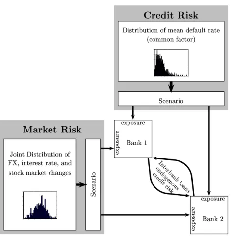
The basic framework is a model of a banking system with a detailed description of the structure of interbank exposures. The model explains the feasible payment flows between banks endoge-nously from a given structure of interbank liabilities, net values of the banks arising from all other bank activities and an assumption about the resolution of insolvency in different states of the world. States of the world are described as follows: We expose the banks financial posi-tions apart from interbank relaposi-tions to interest rate, exchange rate, stock market and business cycle shocks. For each state of the world, the network model uniquely determines endoge-nously actual interbank payment flows. Taking the feedback between banks from mutual credit exposures and mutual exposures to aggregate shocks explicitly into account we can calculate default frequencies of individual banks across states. The endogenously determined vector of feasible payments between banks also determines the recovery rates of banks with exposures to an insolvent counterparty. We are able to distinguish bank defaults that arise directly as a consequence of movements in the risk factors and defaults which arise indirectly because of contagion. The model therefore yields a decomposition into fundamental and contagious de-faults. Our approach is illustrated in Figure 1 which shows the various elements of our risk assessment procedure.

The main data source we use for our model are bank balance sheet data and supervisory data reported monthly to the Austrian Central Bank (Monatsausweis, MAUS). In particular these data give us for each bank in the system an aggregate number of on balance sheet claims

2_{Note that though the term systemic risk belongs to the standard rhetoric of discussions about banking regulation}

it does not have a precise definition (see Summer (2003) for a discussion). We invoke the term here because we think that our approach captures some of the issues frequently discussed under this header, in particular the problem of contagious default.

−6 −4 −2 0 2 4 6 0 5 10 15 20 25 30 ! "#%$&!'(*) +-,.%"/0 "/1 324"/.%2*65 !8739;:<2 "9/=73>62%?/1 @BAC D E F GH 0 1 2 3 4 5 67 8 9 10 0 5 10 15 20 25 N! "#%$&!'O):</02P5&/=)Q2$%RS 324!/ T 7=:<:U;)Q27L! LV W 7=/062* ! XY2*69KZ [!\]&^1_a`b[ cd e fg hi c XY2*69kj ["\]&^0_a`b[ cd e fg hi c lnmLoBp qBrts mu%v w s max p m0y wz p m wQ{ x | q p y} o q } x u

Figure 1. The graph shows the basic structure of the model. Banks are exposed to shocks from credit risk

and market risk according to their respective exposures. Interbank credit risk is endogenously explained by the network model.

and liabilities towards other banks in the system banks abroad and the central bank.3 _From

this partial information we estimate the matrix of bilateral exposures for the entire system. For the estimation of bilateral exposures we can exploit information that is revealed by the sectoral organization of the Austrian banking system.4 _{Scenarios are created by exposing the positions}

on the balance sheet that are not part of the interbank business to interest rate, exchange rate, stock market and loan loss shocks. In order to do so we undertake a historic simulation using market data, except for the loan losses where we employ a credit risk model. In the scenario part we use data from Datastream, the major loans statistics produced at the Austrian Central

3_{Note that these data cover only the on balance sheet part of interbank transactions and do not include off}

balance sheet items.

4_{The sector organization has mainly historic roots and partitions the banks into joint stock banks, savings}

banks, state mortgage banks, Raiffeisen Banks, Volksbanken, construction savings and loans associations and special purpose banks. The system is explained in detail in Section 3.

Bank (Großkreditevidenz, GKE) as well as statistics of insolvency rates in various industry branches from the Austrian rating agency Kreditschutzverband von 1870. For each scenario the estimated matrix of bilateral exposures and the income positions determine via the network model a unique vector of feasible interbank payments and thus a pattern of insolvency. It is the analysis of these data that we rely on to assess the risk exposure of all banks at a system level.5

Using a cross section of data for September 2001 we get the following main results: The Austrian banking system is very stable and default events that could be classified as a ”systemic crisis” are unlikely. We find that the median default probability of an Austrian bank to be below one percent. Perhaps the most interesting finding is that only a small fraction of bank defaults can be interpreted as contagious. The vast majority of defaults is a direct consequence of macroeconomic shocks.6 Furthermore we find the median endogenous recovery rates to be 66%, we show that the Austrian banking system is quite stable to shocks from losses in foreign counterparty exposure and we find no clear evidence that the interbank market either increases correlations among banks or enables banks to diversify risk. Using our model as a simulation tool, we show that market share in the interbank market alone is not a good predictor of the relevance of a bank for the banking system in terms of contagion risk.

1.2

Related Research

To our best knowledge this is the first attempt in the literature to design a framework for the assessment of the risk exposure of an entire banking system taking into account the detailed micro information usually available in central banks.7 _{For the different parts of the model we}

rely on some results in the literature. The network model we use as the basic building block is due to Eisenberg and Noe (2001). These authors give an abstract analysis of a static clearing problem. We rely on these results in the network part of our model. For our analysis we extend this model to a simple uncertainty framework. The idea to recover bilateral interbank exposures using bank balance sheet data has first been systematically pursued by Sheldon and

5_{Why do we treat the vector income positions apart from interbank dealings as state contingent whereas we}

treat the matrix of bilateral exposures as uncontingent? First of all note that the actual interbank payments are in fact not uncontingent because they are determined by the network model and thus interbank payments vary across states of the world. Treating bilateral exposures as state contingent directly with respect to risk factors would mean to have all of them in present values and then to look at consequences of changes in risk factors such as interest rate risk. Such an analysis is not possible - or only at the cost of a set of strong and arbitrary assumptions - for the data we have at the moment. We therefore treat bilateral interbank exposures by looking at given nominal liabilities and claims as we can reconstruct them from the balance sheet data. As shown in Figure 1 we think of this as a model where the income risk of non-interbank positions is driven by exogenous risk factors whereas interbank credit risk is endogenously explained by the network model.

6_{This confirms some of the conclusions drawn in a paper by Kaufman (1994) about the empirical (ir)relevance}

of contagious bank defaults.

7_{There have however been various theoretical attempts to conceptualize such a problem. These papers are Allen}

Maurer (1998) for Swiss data on a sectorally aggregated level. They use an entropy optimization procedure to estimate bilateral exposures from partial information. Upper and Worms (2002) analyze bank balance sheet data for German banks. Applying modern techniques from applied mathematics8_{they are able to deal with a much larger problem than Sheldon and Maurer (1998)}

and estimate bilateral exposures on a entirely disaggregated level.9 _{We use similar methods}

for reconstructing bilateral exposures for the Austrian data. Using disaggregated data has the advantage that much of bilateral exposures can be exactly recovered by exploiting structural information about the banking system under consideration.10 _{The estimation procedure has}

then to be applied only to a relatively small part of exposures for which structural information does not give any guidelines. The credit risk model we use is a version of the CreditRisk+ model of Credit Suisse (1997). We have to adapt this framework to deal with a system of loan portfolios simultaneously rather than with the loan portfolio of a single bank.

There is a related literature that deals with similar questions for payment and banking sys-tems. Humphery (1986) and Angelini, Maresca, and Russo (1996) deal with settlement failures in payment systems. Furfine (2003) and Upper and Worms (2002) deal with banking systems. What is common to all of these studies is that they are concerned with the contagion of de-fault following the simulated failure of one or more counterparties in the system. Our study in contrast undertakes a systematic analysis of risk factors and their impacts on bank income. Bank failures and contagion are studied as a consequence of these economic shocks to the en-tire banking system. Thus while the studies cited above are based on a thought experiment that tries to work out the implications of the structure of interbank lending on the assumed failure of particular institutions our analysis is built on a fully fledged model of the banking system’s risk exposure. The consequences of this exposure are then studied systematically within the frame-work of the netframe-work model. The main innovation of our model is therefore the combination of a systematic scenario analysis for risk factors with an analysis of contagious default. We can of course use our framework to undertake similar simulation exercises as the previous literature on contagious default by letting some institution fail and study the consequences for other banks in the system. Complementing our analysis by such an exercise is interesting because all of the studies cited above get rather different results on the actual importance of contagion effects due to simulated idiosyncratic failure of individual institutions.11

8_{These techniques are outlined in Blien and Graef (1997) as well as in a book by Fang, Rajasekra, and Tsao}

(1997).

9_{Upper and Worms (2002) rely on a combination of exploiting structural information and entropy optimization}

for the reconstruction of bilateral exposures.

10_{This structural information is of course dependent on the country specific features of the reporting systems.}

While we can make use of the fact that many banks have to decompose their reports with respect to certain counterparties (see section 4) Upper and Worms (2002) can use the fact that in Germany banks have to break down their reports between sectors and within this information also with respect to maturities. Since many banks only borrow or lend in the interbank market at specific maturities these authors can identify many bilateral positions.

11_{The study by Humphery (1986) found the contagion potential from settlement failures in the payment system}

to be rather significant. Angelini, Maresca, and Russo (1996) studying settlement failures in the Italian payment system find a low incidence of contagious defaults. Sheldon and Maurer (1998) conclude from their study that

The paper is organized as follows: Section 2 describes the network model of the banking system. Section 3 gives a detailed description of our data. Section 4 explains our estimation procedure for the matrix of bilateral interbank exposures. Section 5 explains our approach to the creation of scenarios. Section 6 contains our simulation results for a cross section of Austrian banks with data from September 2001. Section 7 demonstrates how the framework can be used for thought experiments and contrasts our empirical findings with other results in the literature. The final section contains conclusions. Some of the technical and data details are explained in an appendix.

2

A Network Model of the Interbank Market

The conceptual framework we use to describe the system of interbank credits has been intro-duced to the literature by Eisenberg and Noe (2001). These authors study a centralized static clearing mechanism for a financial system with exogenous income and a given structure of bilateral nominal liabilities. We build on this model and extend it to include uncertainty.

Consider a finite setN ={1, ..., N}of nodes. Each nodei∈ N is characterized by a given incomeeiand nominal liabilitieslijagainst other nodesj ∈ N in the system. The entire system

of nodes is thus described by anN ×N matrixLand a vectore ∈_RN_{. We denote this system}

by the pair(L, e).12

We can interpret the pair(L, e)as a model of a system of bank balance sheets with a detailed description of interbank exposures: Each node i ∈ N in the system corresponds to a bank. The income positions resulting from each bank’s activities is decomposed into two parts: The interbank positions, described byL, and the net wealth position resulting from other activities of the bank.13

Let us illustrate this interpretation of the network model by an example: Consider a system with three banks. The interbank liability structure is described by the matrix

failure propagation due to a simulated default of a single institution is low. Furfine (2003) finds low contagion effects using exact bilateral exposures from Fedwire. Upper and Worms (2002) find potentially large contagion effects once loss rates exceed a certain threshold, estimated by them at around45%.

12_{Note that the liabilities of one nodei∈ N are the claims of some other nodej∈ N.Thus rows are liabilities}

of the nodes whereas columns are claims.

13_{Note that the network description is quite flexible and also allows for a richer interpretation. Some banks in} N could for instance describe the central bank or the world outside the banking system. One could also append to the system a node that Eisenberg and Noe (2001) call the ”sink node”. It has aneiof zero and no obligations to other banks. Liabilities of banks to employees, to the tax authorities etc. can then be viewed as claims of this node to the system.

L=   0 0 2 3 0 1 3 1 0   (1)

In our example, bank3has - for instance - liabilities of3with bank1and liabilities of1with bank2. It has of course no liabilities with itself. The total interbank liabilities for each bank in the system is given by a vector d = (2,4,4). With actual balance sheet data the components of the vectordcorrespond to the position due to banks for bank1, 2and3respectively. If we alternatively look at the column sum ofLwe get the position due from banks. Assume that we can summarize the net wealth of the banks that is generated from all other activities by a vector e = (1,1,1). This vector corresponds to the difference of asset positions such as bonds, loans and stock holdings and liability positions such as deposits and securitized liabilities.

To determine feasible payments between banks we have to say something about situations where a bank is not able to honor its interbank promises. To make liabilities and claims mutually consistent a simple mechanism to resolve situations of insolvency is in place. This clearing mechanism is basically a redistribution scheme. If the total net value of a bank - i.e. the income received from other banks plus the income position of non interbank activities minus the bank’s own interbank liabilities - becomes negative, the bank is insolvent. In this case the claims of creditor banks are satisfied proportionally. This is a stylized and simplified description of a bankruptcy procedure. In this procedure the following properties are taken into account: Banks have limited liability and default is resolved by proportional sharing of the value of the debtor bank among it’s creditor banks. Therefore the exogenous parameters(L, e) together with the assumption about the resolution of insolvency endogenously determine the actual payments between banks.

In Eisenberg and Noe (2001) these ideas are formalized as follows: Denote byd∈_RN

+14the

vector of total obligations of banks towards the rest of the system i.e., we havedi =P_j∈Nlij.

Proportional sharing of value in case of insolvency is described by defining a new matrixΠ ∈

[0,1]N×N. This matrix is derived from Lby normalizing the entries by total obligations. We write:

πij =

lij

di ifdi >0

0 otherwise (2)

With these definitions we can describe a financial system with a clearing mechanism that respects limited liability of banks and proportional sharing as a tuple (Π, e, d) ∈ [0,1]N×N _×

14

RN ×RN+ for which we explain endogenously a so called clearing payment vectorp

∗ _∈

RN+. It

denotes the total payments made by the banks under the clearing mechanism. We have:

Definition 1 A clearing payment vector for the system(Π, e, d) ∈ [0,1]N×N ×_RN _×

RN+ is a

vectorp∗ ∈ ×N

i=1[0, di]such that for alli∈ N

p∗_i = min[di,max( N X

j=1

πjip∗j +ei,0)] (3)

Applied to our example the normalized liability matrix is given by

Π =   0 0 1 3 4 0 1 4 3 4 1 4 0  

For an arbitrary vector of actual paymentspbetween banks the net values of banks can then be written as

ΠTp+e−p

Under the clearing mechanism - given the payments of all counterparties in the interbank market - a bank either honors all it’s promises and paysp∗_i =di or it is insolvent and pays

p∗_i = max(

N X

j=1

πjip∗j +ei,0) (4)

The clearing payment vector thus directly gives us two important insights. First: For a given structure of liabilities and bank values(Π, e, d)it tells us which banks in the system are insolvent. Second: It tells us the recovery rate for each defaulting bank in each state.

To find a clearing payment vector we have to find a solution to a system of inequalities. Eisenberg and Noe (2001) prove that under mild regularity conditions a unique clearing pay-ment vector for(Π, e, d)always exists. These results extend - with slight modifications - to our framework as well.15

The clearing algorithm contains even more information that is interesting for the assessment of credit risk in the interbank market and for issues of systemic stability. This can be seen by an explanation of the method by which we calculate clearing payment vectors. This method is due to Eisenberg and Noe (2001). They call their procedure the ”fictitious default algorithm”.

15_{In Eisenberg and Noe (2001) the vectoreis in}

This term basically describes what is going on in the calculation. For a given (Π, e, d) the procedure starts under the assumption that all banks fully honor their promises, i.e. p∗ = d. If under this assumption all banks have positive value, the procedure stops. If there are banks with a negative value, they are declared insolvent and the clearing mechanism calculates their payment according to the clearing formula (4) and keeps the payments of the positive value banks fixed. Now it can happen that banks that had a positive value in the first iteration have a negative value in the second because they loose on their claims on the insolvent banks. Then these banks have to be cleared and a new iteration starts. Eisenberg and Noe (2001) prove that this procedure is well defined and converges after at most N steps to the unique clearing payment vectorp∗.16

This procedure thus generates interesting information in the light of systemic stability. A bank that is insolvent in the first round of the fictitious default algorithm is fundamentally in-solvent. Bank defaults in consecutive rounds can be considered as contagious defaults.17

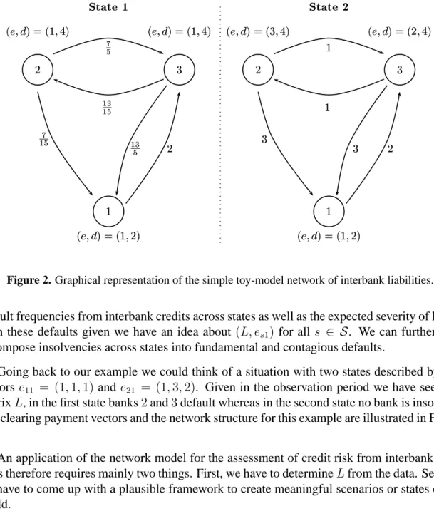
An application of the fictitious default algorithm to our example leads to a clearing payment vector of p∗ = (2,28₁₅,52₁₅). It is easy to check that bank2 is fundamentally insolvent whereas bank3is “dragged into insolvency“ by the default of bank2.

To extend the model of the clearing system to a simple uncertainty framework we work with a basic event tree. Assume that there are two dates t = 0 and t = 1.Think of t = 0as the observation period, where (L, e0) is observed. Then economic shocks affect the income

vector e0. The shocks lead to a realization of one state s in a finite set S of states of the

world att = 1. Each state is characterized by a particulares1.Think oft = 1as a hypothetical

clearing date where all interbank claims are settled according to the clearing mechanism. By the theorem of Eisenberg and Noe (2001) we know that such a clearing payment vector is uniquely determined for each pair (L, es1). Thus from an ex-ante perspective we can assess expected 16_{Note that our setup implicitly contains a seniority structure of different debt claims of banks. By interpreting} eias net income from all bank activities except the interbank business we assume that interbank debt claims are junior to other claims, like depositors or bond holders. However interbank claims have absolute priority in the sense that the owners of the bank get paid only after all debts have been paid. In reality the legal situation is much more complicated and the seniority structure might very well differ from the simple procedure we employ here. For our purpose it gives us a convenient simplification that makes a rigorous analysis of interbank defaults tractable.

17_{At this point it is perhaps useful to point out that the clearing payment vector is a fixed point of the map} ×N

i=1[0, d

i_{] → ×}N i=1[0, d

i_{],p 7→ ((Π}T_{p+e)∨0)∧dwhereas the dynamic interpretation is derived from the}

iterative procedure by which the fixed point is actually calculated. We therefore hesitate to follow Eisenberg and Noe (2001) by interpreting insolvencies at later rounds of the fictitious default algorithm as indicating higher “systemic stability“ of a bank. Of course one can define such a measure. Since there are other ways to calculate the clearing payment vector, the order of rounds in the fictitious default algorithm does not have a meaningful economic interpretation. The fictitious default algorithm nevertheless allows for a meaningful decomposition between defaults directly due to shocks or indirectly due to default of other banks in the system. No matter how the clearing vector is calculated the interpretation of fundamental insolvency has a clear economic interpretation and the classification of all other defaults as contagious does not depend on the particular calculation procedure, i.e. the fictitious default algorithm.

%

Figure 2. Graphical representation of the simple toy-model network of interbank liabilities.

default frequencies from interbank credits across states as well as the expected severity of losses from these defaults given we have an idea about (L, es1) for all s ∈ S. We can furthermore

decompose insolvencies across states into fundamental and contagious defaults.

Going back to our example we could think of a situation with two states described by two vectorse11 = (1,1,1)and e21 = (1,3,2). Given in the observation period we have seen the

matrixL, in the first state banks2and3default whereas in the second state no bank is insolvent. The clearing payment vectors and the network structure for this example are illustrated in Figure 2.

An application of the network model for the assessment of credit risk from interbank posi-tions therefore requires mainly two things. First, we have to determineLfrom the data. Second, we have to come up with a plausible framework to create meaningful scenarios or states of the world.

3

The Data

In the following we give a short description of our data. Our main sources are bank balance sheet and supervisory data from the Monatsausweis (MAUS) database of the Austrian Central

Bank (OeNB) and the database of the OeNB major loans register (Großkreditevidenz,GKE). We use furthermore data on default frequencies in certain industry groups from the Austrian rating agency Kreditschutzverband von 1870. Finally we use market data from Datastream.

3.1

The Bank Balance Sheet Data

Banks in Austria report balance sheet data to the central bank on a monthly basis18_{. On top}

of balance sheet data MAUS contains a fairly extensive amount of other data that are relevant for supervisory purposes. They include among others numbers on capital adequacy statistics on times to maturity and foreign exchange exposures with respect to different currencies. We can use this information to learn more about the structure of certain balance sheet positions.

In our analysis we use a cross section from the MAUS database for September 2001 which we take as our observation period. We want to use these data to get an estimate of the matrix Las well as to determine the vectore0. All items are broken down in Euro exposures and into

foreign exchange exposures.

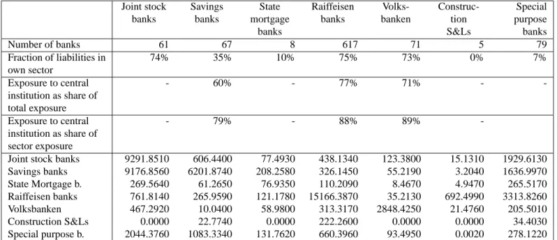
A particular institutional feature of the Austrian banking system helps us with the estimation of bilateral interbank exposures. It has a sectoral organization for historic reasons. Banks belong to one of the seven sectors: joint stock banks, savings banks,state mortgage banks, Raiffeisen banks, Volksbanken, housing construction savings and loan associations and special purpose banks. This sectoral organization of banks left traces in the data requirements of OeNB. Banks have to break down their MAUS reports on claims and liabilities with other banks according to the different banking sectors, central bank and foreigners. This practice of reporting on bal-ance interbank positions reveals some structure of the L matrix. The savings banks and the Volksbanken sector are organized in a two tier structure with a sectoral head institution. The Raiffeisen sector is organized by a three tier structure, with a head institution for every federal state of Austria. The federal state head institutions have a central institution, Raiffeisenzentral-bank (RZB) which is at the top of the Raiffeisen structure. Banks with a head institution have to disclose their positions with the head institution. This gives us additional information on L. From the viewpoint of banking activities the sectoral organization is today not particularly relevant. The activities of the sectors differ only slightly and only a few banks are specialized in specific lines of business. The908independent banks in our sample are to the largest extent universal banks.

Total assets in the Austrian banking sector in September 2001 were567,071Million Euro. The sectoral shares are: 22% joint stock banks,35% savings banks,6%state mortgage banks, 21%Raiffeisen banks,5%Volksbanken,3%housing construction savings and loan associations and8%special purpose banks. The banking system is dominated by a few big institutions: 57%

18_{This report called Monatsausweis (MAUS) is regulated in§74 Abs. 1 and 4 of the Austrian banking law,}

Joint stock banks Savings banks State mortgage banks Raiffeisen banks Volks-banken Construc-tion S&Ls Special purpose banks Number of banks 61 67 8 617 71 5 79 Fraction of liabilities in own sector 74% 35% 10% 75% 73% 0% 7% Exposure to central institution as share of total exposure - 60% - 77% 71% - -Exposure to central institution as share of sector exposure - 79% - 88% 89%

-Joint stock banks 9291.8510 606.4400 77.4930 438.1340 123.3800 15.1310 1929.6130 Savings banks 9176.8560 6201.8740 208.2580 326.1450 55.2190 3.2040 1636.9970 State Mortgage b. 269.5640 61.2650 76.9350 110.2090 8.4670 4.9470 265.5170 Raiffeisen banks 761.8140 265.9590 121.1780 15166.3870 35.2130 692.4990 3313.8260 Volksbanken 467.2920 10.0400 58.9800 313.3170 2848.4250 21.4760 205.5010 Construction S&Ls 0.0000 22.7740 0.0000 222.2600 0.0000 0.0000 34.4030 Special purpose b. 2044.3760 1083.3340 131.7620 660.3960 93.4950 0.0020 278.1220

Table 1. Sectoral decomposition of interbank liabilities. The table shows the number of banks in each

sector, the average fraction of interbank liabilities towards banks in the own sector as share of total exposure, the average fraction of interbank liabilities towards banks in the own sector as share of their sector exposure as well as the average liability of sectorally organized banks with their head institution. The first row in the lower block shows liabilities of joint stock banks against joint stock banks, of joint stock banks against savings banks etc.. The next row is to be read in the same way. These numbers are in Million Euro.

of total assets are concentrated with the10biggest banks. The share of total interbank liabilities in total assets of the banking system is33%.

Statistics for the data on domestic interbank exposures are displayed in Table 1, which shows sectoral aggregates of the domestic on balance sheet exposures for the Austrian interbank market. About two thirds of all Austrian banks belong to the Raiffeisen sector which consists mainly of small, independent banks in rural areas. From the fraction of liabilities in the own sector we can see that some sectors form a fairly closed system, where the average bank holds about three quarters of the liabilities within the sector. Construction S&Ls have no liabilities to banks in their sector. We can also see that banks in a sector with a head institution do the major share of their interbank activities with their own head institution. This is in particular true for many of the smaller banks. The special purpose banks are quite diversified in their liabilities.

3.2

The Credit Exposure Data

We can get a rough breakdown for the banks’ loan portfolio to non-banks by making use of the major loans register of OeNB (Großkreditevidenz, GKE). This database contains all loans exceeding a volume of364,000Euro. For each bank we use the amount of loans to enterprises from 35sectors classified according to the NACE standard.19 _{It gives us the volume as well}

as the number of credits to these different industry branches. Combining this information with data from the Austrian Rating Agency Kreditschutzverband von 1870 (KSV) we can estimate the riskiness of a loan in a certain industry. The KSV database gives us time series of default rates for the different NACE branches. From this statistics we can produce an average default frequency and its standard deviation for each NACE branch. These data serve as our input to the credit risk model.20

For the part of loans we can not allocate to industry sectors we have no default statistics and no numbers of loans. To construct an insolvency statistics for the residual sector we take averages from the data that are available. To construct a number of loans figure for the residual sector we assume the share of loan numbers in industry and in the residual sector is proportional to the share of loan volume between these sectors. We have chosen this approach for a lack of better alternatives. We should also note that the insolvency series is very short. The series are available semi-annually beginning with January 1997 which gives us8observations per sector. Thus the estimate of mean default rates and their standard deviation we can get from these data is noisy.21 We display average default frequencies and their standard deviation that we get from these data in Table 10 in Appendix A.

3.3

Market Data

Some positions on the banks’ asset portfolios are subject to market risk. We collect market data corresponding to the exposure categories over twelve years from September 1989 to September 2001 from Datastream. These data are used for the creation of scenarios. Specifically we collect exchange rates of USD, JPY, GBP and CHF to the Austrian Schilling (Euro) to compute

19_{We use the classification according to ¨ONACE 1995. This is the Austrian version of NACE Rev. 1 , a European}

classification scheme, which has to be applied according to VO (EWG) Nr. 3037/ 90 for all member states. NACE is an acronym for Nomenclature g´en´erale des activit´es ´economiques dans les communaut´es europ´eennes.

20_{The matching procedure we apply suffers from some data inconsistencies. Though the data come in principle}

from the same sources the reporting procedures are not rooted in exactly the same legal base. So there might be discrepancies in the numbers. MAUS is legally based on the Austrian law on banking, Bankwesengesetz (BWG) whereas the legal base for GKE is the BWG plus a special regulation for loans with volume above a certain threshold (Großkreditmeldungsverordnung GKMVO).

21_{In particular the data don’t contain a business cycle. Again we have to live with this short series because this is}

the most we can get at the moment. These estimates will become better in the future however as more observations are collected.

exchange rate risk. As we only have data on domestic and international equity exposure we include the Austrian index ATX and the MSCI-world index in our analysis. To account for interest rate risk, we compute zero bond prices for three month, one, five and ten years, from collected zero rates for EUR, USD, JPY, GBP and CHF.22

4

Estimating Interbank Liabilities from Partial Information

If we want to apply the network model to our data we have the problem that they contain only partial information about the interbank liability matrixL. The bank by bank record of assets and liabilities with other banks gives us the column and row sums of the matrixL. Furthermore we know some structural information. For instance we know that the diagonal ofL(and thus of Π) must contain only zeros since banks do not have claims and liabilities against themselves.

The sectoral structure of the Austrian banking system gives us additional information we can exploit for the reconstruction of the Lmatrix. The bank records contain claims and liabilities against the different sectors. Hence we know the column and row sums of the submatrices of the sectors. Two sectors have a two tier and one sector has a three tier structure. Banks in these sectors break down their reports further according to the amount they hold with the central institution. Due to the fact that there are many banks that hold all their claims and liabilities within their sector or only against the respective central institution these pieces of information determine already72%of all entries of the matrixLexactly. Therefore by exploiting the sectoral

information, we actually know a major part ofLfrom our data.

We would like to estimate the remaining 28% of the entries of Lby optimally exploiting the information we have. Our ignorance about the unknown parts of the matrix should be reflected in the fact that all these entries are treated uniformly in the reconstruction process. The procedure should be furthermore adaptable to include any new information that might get available in the process of data collection. In the following we use a procedure that formulates the reconstruction of the unknown parts of theLmatrix as an entropy optimization problem.23

22_{Sometimes a zero bond series is not available for the length of the period we need for our exercise. In these}

cases we took swap rates.

23_{This procedure has been applied already to the problem of reconstructing unknown bilateral interbank}

expo-sures from aggregate information by Upper and Worms (2002) and Sheldon and Maurer (1998). Entropy optimiza-tion is applied in a wide range of practical problems. For a detailed descripoptimiza-tion see Fang, Rajasekra, and Tsao (1997) or Blien and Graef (1997). As we have explained above entropy optimization can be justified on informa-tional grounds. There are counterarguments to this as well. One might criticize that entropy optimization is not a very attractive procedure for the risk analysis of our paper because it makes exposures maximally diversified among the unknown cells ofLand one would presumably be much more interested in extremer structures. On the other hand our knowledge about ’critical’ liability structures is at the moment very poor and any assumption would be even more arbitrary than the entropy procedure. We should however stress that these considerations are not so important for our case since we are able to identify a very large set of entries inLexactly. Thus it is the

What this procedure does can intuitively be explained as follows: It finds a matrix that fulfills all the constraints we know of and treats all other parts of the matrix as balanced as possible. This can be formulated as minimizing a suitable measure of distance between the estimated matrix and a matrix that reflects our a priori knowledge on large parts of bilateral exposures. It turns out that the so called cross entropy measure is a suitable concept for this task (see Fang, Rajasekra, and Tsao (1997) or Blien and Graef (1997)).

Assume we have in totalKconstraints that include all constraints on row and column sums as well as on the value of particular entries. Let us write these constraints as

N X i=1 N X j=1 akijlij =bk (5)

fork= 1, ..., K andakij ∈ {0,1}.

We want to find the matrixLthat has the least discrepancy to some a priori matrixU with respect to the (generalized) cross entropy measure

C(L, U) = N X i=1 N X j=1 lijln( lij uij ) (6)

among all the matrices fulfilling (5) with the convention that lij = 0 whenever uij = 0 and

0 ln(0₀)is defined to be0.

Due to data inconsistencies the application of entropy optimization is not straightforward. For instance the liabilities of all banks in sectork against all banks in sectorl do typically not equal the claims of all banks in sectorl against all banks in sectork.24 _{We solve this problem}

by using constructing a start matrix for the entropy maximization, which reflects all our a priory knowledge. The procedure is described in detail in Appendix B

We see three main advantages of this method to deal with the incomplete information prob-lem raised by our data. First the method is able to include all kinds of constraints we might find out about the matrixL maybe from different sources. Second, as more information becomes available the approximation can be improved. Third, there exist computational procedures that are easy to implement and that can deal efficiently with very large problems (see Fang, Ra-jasekra, and Tsao (1997) or Blien and Graef (1997)). Thus problems similar to ours can be solved efficiently and quickly on an ordinary personal computer, even for very large banking systems.

combination of structural knowledge plus entropy optimization which gives the estimation of bilateral exposures some bite.

24_{We do not know the reasons for these discrepancies. Some of the inconsistencies seem to suggest that the}

5

Creating Scenarios

Our model of the banking sector uses different states of the world or scenarios to model uncer-tainty. In each scenario banks face gains and losses due to market risk and credit risk. Some banks may fail which possibly causes subsequent failures of other banks, as it is modeled in our network clearing framework. In our approach the credit risk in the interbank network is modeled endogenously while all other risks - like gains and losses from FX and interest rate changes as well as from equity price changes losses from loans to non-banks - are reflected in the position ei. The perspective taken in our analysis is to ask, what are the consequences of

different scenarios foreion the whole banking system.

We choose a standard risk management framework to model the shocks to banks. To simu-late scenario losses that are due to exposures to market risk we conduct a historical simulation and to capture losses from loans to non-banks we use a credit risk model.

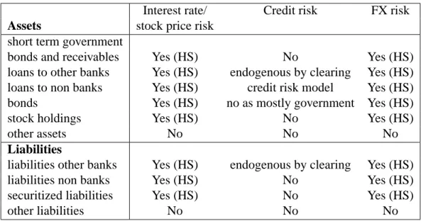
Table 2 shows, which balance sheet items are included in our analysis and how the risk exposure is modeled. Market risk (stock price changes, interest rate movements and FX rate shifts) are captured by a historical simulation approach (HS) for all items except other assets and other liabilities, which includes long term major equity stakes in not-listed companies, non financial assets like property and IT-equipment and cash on the asset side and equity capital and provisions on the liability side. Credit losses from non-banks are modeled via a credit risk model. The credit risk from bonds is not included since most banks hold only government bonds. The credit risk in the inter-bank market is determined endogenously.

5.1

Market Risk: Historical Simulation

We use a historical simulation approach as it is documented in the standard risk management literature (Jorion (2000)) to assess the market risk of the banks in our system. This methodology has the advantage that we do not have to specify a certain parametric distribution for our returns. Instead we can use the empirical distribution of past observed returns and thus capture also extreme changes in market risk factors. From the return series we draw random dates. By this procedure we capture the joint distribution of the market risk factors and thus take correlation structures between interest rates, stock markets and FX markets into account.

To estimate shocks on bank capital stemming from market risk, we include positions in foreign currency, equity and interest rate sensitive instruments. For each bank we collect foreign exchange exposures for USD, JPY, GBP and CHF only as no bank in our sample has open positions of more than1%of total assets in any other currency. From the MAUS database we get exposures to foreign and domestic stocks, which is equal to the market value of the net position held in these categories. The exposure to interest rate risk can not be read directly from the banks’ monthly reports. We have information on net positions in all currencies combined

Interest rate/ Credit risk FX risk

Assets stock price risk

short term government

bonds and receivables Yes (HS) No Yes (HS) loans to other banks Yes (HS) endogenous by clearing Yes (HS) loans to non banks Yes (HS) credit risk model Yes (HS) bonds Yes (HS) no as mostly government Yes (HS)

stock holdings Yes (HS) No Yes (HS)

other assets No No No

Liabilities

liabilities other banks Yes (HS) endogenous by clearing Yes (HS) liabilities non banks Yes (HS) No Yes (HS) securitized liabilities Yes (HS) No Yes (HS)

other liabilities No No No

Table 2. The table shows how risk of the different balance sheet positions is covered in our scenarios.

HS is a shortcut for historic simulation.

for different maturity buckets (up to 3 month but not callable, 3 month to 1 year, 1 to 5 years, more than 5 years). These given maturity bands allow only a quite coarse assessment of interest rate risk.25 Nevertheless the available data allow us to estimate the impact of changes in the term structure of interest rates. To get an interest rate exposure for each of the five currencies EUR, USD, JPY, GBP and CHF we split the aggregate exposure according to the relative weight of foreign currency assets in total assets. This procedure gives us a vector of 26exposures, 4 FX,2equity, and 20interest rate, for each bank. Thus we get aN ×26matrix of market risk exposure.

We collect daily market prices over3,219 trading days for the risk factors as described in subsection 3.3. From the daily prices of the26risk factors we compute daily returns. We rescale these to monthly returns assuming twenty trading days and construct a26×3219matrixRof monthly returns.

25_{We would like to have a finer granularity in the buckets, because right now a wide range of maturities is}

grouped together. We would prefer more buckets especially in the longer maturities. As the maturity buckets in the banks’ exposure reports are quite broad, there will be instruments of different maturities in each bucket. As we consider only the net position within each bucket for our risk analysis, we might have some undesired netting effects that will result in an underestimation of market risk. Consider for example a five year loan that is financed by one year deposits. As both assets fall into the same bucket, the net exposure is zero despite of the fact that there is some obvious interest rate risk. We compensate for this effect by choosing as risk factors for each bucket a zero bond with a maturity at the upper bound of the respective maturity band.

For the historical simulation we draw 10,000 scenarios from the empirical distribution of returns. To illustrate the procedure letRs be one such scenario, i.e. a column vector from the

matrixR. Then the profits and losses that arise from a change in the risk factors as specified by the scenario are simply given by multiplying them with the respective exposures. Let the exposures that are directly affected by the risk factors in the historical simulation be denoted bya. The vectoraRs contains then the profits or losses each bank realizes under the scenario

s ∈ S. Repeating the procedure for all 10,000 scenarios, we get a distribution of profits and losses due to market risk.

5.2

Credit Risk: Calculating Loan Loss Distributions

For the modeling of loan losses we can not apply a historical simulation as there are no published time series data on loan defaults. We employ one of the standard modern credit risk models -CreditRisk+ - to estimate a loan loss distribution for each bank in our sample.26 We rely on this estimated loss distribution to create for each bank the loan losses across scenarios. While CreditRisk+ is designed to deal with a single loan portfolio we have to deal with a system of portfolios since we have to consider all banks simultaneously. The adaptation of the model to deal with such a system of loan portfolios turns out to be straightforward.

The basic inputs CreditRisk+ needs to calculate a loss distribution is a set of loan exposure data, the average number of defaults in the loan portfolio of the bank and its standard deviation. Aggregate shocks are captured by estimating a distribution for the average number of loan defaults for each bank.27 _{This models business cycle effects on average industry defaults. The}

idea is that these default frequencies increase in a recession and decrease in booms. Given this common shock, defaults are assumed to be conditionally independent. We construct the bank loan portfolios by decomposing the bank balance sheet information on loans to non banks into volume and number of loans in different industry sectors according to the information from the major loan register. The rest is summarized in a residual position as described in Section 3. Using the KSV insolvency statistics for each of the 35 industry branches and the proxy insolvency statistics for the residual sector, we can assign an average default frequency and a standard deviation of this frequency to the different industry sectors. The riskiness of a loan in a particular industry is then assumed to be described by these parameters. Based on this information we can calculate the average default frequency and it’s standard deviation for each individual bank portfolio. From these data we then construct the distribution of the aggregate shock (i.e. the average default frequency of the bank portfolio), for each bank in our sample.

26_{A recent overview on different standard approaches to model credit risk is Crouhy, Galai, and Mark (2000).}

CreditRisk+ is a trademark of Credit Suisse Financial Products (CSFP). It is described in detail in CSFP Credit Suisse (1997)

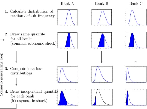
27_{In CreditRisk+ this distribution is specified as a gamma distribution. The parameters of the gamma distribution}

Bank A Bank B Bank C 0 200 400 600 800 1000 1200 0 0.5 1 1.5 2 2.5 3 3.5x 10−3 0 200 400 600 800 1000 1200 1400 0 0.5 1 1.5 2 2.5x 10−3 0 50 100 150 200 250 300 0 0.002 0.004 0.006 0.008 0.01 0.012 0.014 1. _{Calculate distribution of} median default frequency

0 200 400 600 800 1000 1200 0 0.5 1 1.5 2 2.5 3 3.5x 10−3 0 200 400 600 800 1000 1200 1400 0 0.5 1 1.5 2 2.5x 10−3 0 50 100 150 200 250 300 0 0.002 0.004 0.006 0.008 0.01 0.012 0.014

2. _{Draw same quantile} for all banks

(common economic shock)

0 10 20 30 40 50 60 70 80 0 0.005 0.01 0.015 0.02 0.025 0.03 0.035 0.04 0.045 0.05 0 20 40 60 80 100 120 140 160 0 0.002 0.004 0.006 0.008 0.01 0.012 0.014 0.016 0.018 0.02 0 10 20 30 40 50 60 70 0 0.02 0.04 0.06 0.08 0.1 0.12

3. _{Compute loan loss} distributions 0 10 20 30 40 50 60 70 80 0 0.005 0.01 0.015 0.02 0.025 0.03 0.035 0.04 0.045 0.05 0 20 40 60 80 100 120 140 160 0 0.002 0.004 0.006 0.008 0.01 0.012 0.014 0.016 0.018 0.02 0 10 20 30 40 50 60 70 0 0.02 0.04 0.06 0.08 0.1 0.12

4. _{Draw independent quantile} for each bank

(ideosyncratic shock)

Scenario

generating

lo

op

Figure 3. Computation of Credit loss scenarios following an extended CreditRisk+ model. Based on

the composition of the individual bank’s loan portfolio we estimate the distribution of the mean default rate for each bank (step 1). Reflecting the idea of a common economic shock we draw the same quantile from each bank’s mean default rate distribution (step 2). Based on this draw, we can compute each bank’s individual loan loss distribution (step 3). The scenario loan losses are then drawn independently for each bank to reflect an idiosyncratic shock (step 4). 10,000 scenarios are drawn repeating steps 2 to 4.

With these data we are now ready to create loan loss scenarios. First we draw for each bank a realization from each bank’s individual distribution of average default frequencies. To model this as an economy wide shock, we draw the same quantile for all banks in the banking system. Given the average default frequency, defaults are assumed to be conditionally independent. We can then calculate a conditional loss distribution for each bank, from which we then draw loan losses.28 Figure 3 illustrates the procedure for scenario generation in our extended CreditRisk+ framework.

28_{We apply standard variance reduction techniques in our Monte Carlo simulation. We go through the quantiles}

of the distribution of average default frequencies at a step length of0.01. Thus, we draw hundred economy wide shocks from each of which we draw 100 loan loss scenarios, yielding a total number of 10,000 scenarios.

Minimum 10% Quantile Median 90%Quantile Maximum

Joint stock banks 0% 0% 0.02% 3.70% 69.00%

Savings banks 0% 0.01% 0.27% 2.80% 7.43%

State Mortgage banks 0% 0.01% 0.42% 2.16% 2.64%

Raiffeisen banks 0% 0.01% 0.97% 13.50% 72.57%

Volksbanken 0% 0.01% 0.33% 7.19% 84.75%

Construction S&Ls 0.09% 0.088% 6.05% 13.46% 13.46%

Special purpose banks 0% 0% 0% 0.69% 34.61%

Entire banking system 0% 0% 0.51% 10.68% 84.75%

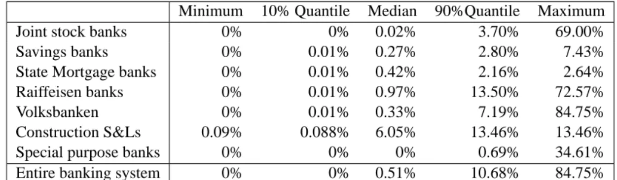
Table 3. Default probabilities of individual banks, grouped by sectors and for the entire banking system.

5.3

Combining Market Risk, Credit Risk, and the Network Model

The credit losses across scenarios are combined with the results of the historic simulations to create the total scenarios fores for each bank. By the network model the interbank payments

for each scenario are then endogenously explained by the model for any given realization ofes

(see Figure 1). Thus we get endogenously a distribution of clearing vectors, default frequencies, recovery rates and a statistics on the decomposition into fundamental and contagious defaults.

6

Results

6.1

Default frequencies

From the network model we get a distribution of clearing vectorsp∗ and therefore also a dis-tribution of insolvencies for each individual bank across states of the world. This is because whenever a component in p∗ is smaller than the corresponding component ind the bank has not been able to honor it’s interbank promises. We can thus generate a distribution of default frequencies for individual sectors and for the banking system as a whole. The relative frequency of default across states is then interpreted as a default probability. The distribution of default probabilities is described in Table 3. It shows minimum, maximum the 10 and 90 percent quan-tiles as well as the median of individual bank default probabilities grouped by sectors and for the entire banking system.

We can see from the table that some banks are extremely safe as default probabilities in the 10 percent quantile are very low and often even zero. Also the median default probability is below 1 percent for every sector except the Construction S&Ls. Default probabilities increase as we go to the 90% quantile but they stay fairly low. Very few banks however have a very high probability of default. For a supervisor, running this model such banks could be identified from

Minimum 10% Quantile Median 90%Quantile Maximum

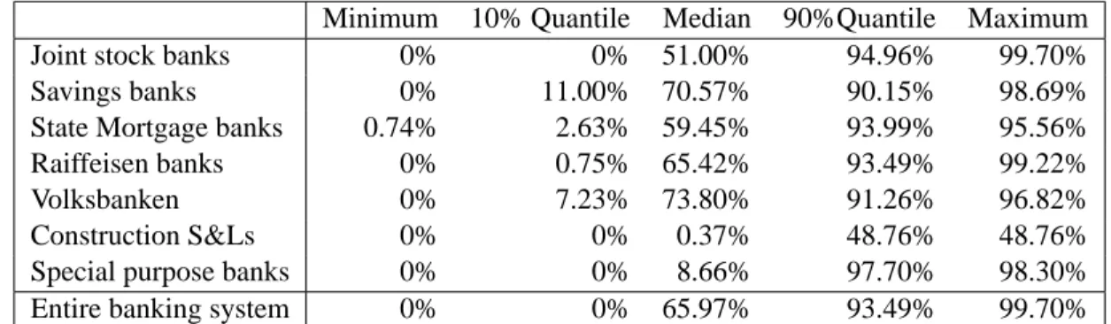
Joint stock banks 0% 0% 51.00% 94.96% 99.70%

Savings banks 0% 11.00% 70.57% 90.15% 98.69%

State Mortgage banks 0.74% 2.63% 59.45% 93.99% 95.56%

Raiffeisen banks 0% 0.75% 65.42% 93.49% 99.22%

Volksbanken 0% 7.23% 73.80% 91.26% 96.82%

Construction S&Ls 0% 0% 0.37% 48.76% 48.76%

Special purpose banks 0% 0% 8.66% 97.70% 98.30%

Entire banking system 0% 0% 65.97% 93.49% 99.70%

Table 4. Individual bank recovery rates of interbank credits grouped by sectors and for the entire banking

system.

our calculations and looked at more closely to get a more precise idea, of what the problem might be.

6.2

Severity of losses: Recovery rates

For the severity of a crisis of course default frequencies are not the only thing that counts. We also want to judge the severity of losses. An advantage of the network model is that it yields for each bank endogenous recovery rates, i.e. the fraction of actual payments relative to promised payments in the case of default.29 Of course these recovery rates must not be taken literally because they are generated by the clearing mechanism of the model under very specific assumptions. If in reality a bank would become insolvent and sent into bankruptcy, bankruptcy costs or other sharing rules than assumed in this paper could affect recovery rates. However the network model can give a good impression on the order of magnitudes that might be available in such an event. We report expected recovery ratios in Table 4.

As we can see, the median recovery rate in the banking system is 66%. Thus for more than half of the banks in the entire banking system the value of their interbank claims is not reduced by more than a third in case of default of a counterparty. If we look at the sectoral grouping of the median recovery rate we see substantial differences. While savings banks and Volksbanken have median recovery rates above 70%, the median recovery rate for the Construction S&Ls is very low.

29_{In terms of the network model, it is the ratio}p∗_i

di∀i∈ N with0≤p

∗

6.3

Systemic stability: Fundamental versus Contagious Defaults

Let us now turn to the decomposition into fundamental and contagious defaults. This decompo-sition is particularly interesting from the viewpoint of systemic stability. It is also interesting to get an idea about contagion of bank defaults from a real dataset since the empirical importance of domino effects in banking has been controversial in the literature.30 _{Bank defaults may be}

driven by large exposures to market and credit risk or from an inadequate equity base. Bank defaults may however also be initiated by contagion: as a consequence of a chain reaction of other bank failures in the system. The fictitious default algorithm allows us to distinguish these different cases.

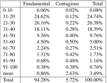
Non-contagious bank defaults lead to insolvency in the first round of the fictitious default algorithm. These defaults are a direct result from shocks to fundamental risk factors of the banks’ businesses. As the iterations of the algorithm increase other banks may become insolvent as a result of bank failures elsewhere in the system. These cases may be classified as contagious defaults. These risks are not visible by a regulatory setup that focuses on individual banks’ ”soundness”. Table 5 summarizes the probabilities of fundamental and contagious defaults in our data.

We list the probabilities of 0−10 banks defaulting fundamentally and the probability of banks defaulting contagiously as a consequence of this event. The next row shows similar in-formation for the event that 11−20banks get insolvent and the probability that other banks default contagiously as a consequence of this etc. What is remarkable in this table is that the relative importance of contagious default events as compared to the importance of contagious defaults is relatively low. In fact approximately94%of default events are directly due to move-ments in risk factors whereas6%can be classified as contagious.

The number of default cases by its own does not provide a full picture of the effects of insolvency. It is interesting to look also at the size of institutions that are affected. Describing bank size by total assets, we see that the average bank affected by fundamental default holds 0.8%of the assets in the banking system. In the worst case of our scenarios we find that banks holding38.9%of the assets in the banking system default fundamentally. Looking at contagious defaults across all scenarios total assets of banks affected are on average0.05%, whereas in the worst scenario banks with a share of 36.9% in total assets are affected. In total we have the numbers 0.9% and 37%. Plotting a histogram of bank defaults by total assets confirms the picture we get from this statistics. Smaller banks are more likely to fail than the larger banks as we can see in Figure 4.

Our finding that the risk of contagion is relatively small is in line with findings in Furfine (2003). Upper and Worms (2002), letting one bank fail at a time, find that, while the average contagion effect following the simulated default of a single institution, is small, the maximum

Fundamental Contagious Total 0-10 6.06% 0.02% 6.08% 11-20 24.62% 0.12% 24.74% 21-30 26.16% 0.22% 26.38% 31-40 18.11% 0.28% 18.39% 41-50 9.36% 0.40% 9.76% 51-60 4.50% 0.50% 5.00% 61-70 2.24% 0.27% 2.51% 71-80 1.31% 0.42% 1.73% 81-90 0.68% 0.48% 1.16% 91-100 0.38% 0.38% 0.76% more 0.86% 2.63% 3.49% Total 94.28% 5.72% 100.00%

Table 5. Probabilities of fundamental and contagious defaults. A fundamental default is due to the losses

arising from exposures to market risk and credit risk to the corporate sector, while a contagious default is triggered by the default of another bank who cannot fulfill its promises in the interbank market.

0 50000 100000 150000 200000 250000 0 0.1 0.2 0.3 0.4 0.5 0.6 0.7 0.8 0.9 Total Assets Frequency

contagion effect increases steeply once the loss ratio has exceeded a critical threshold of about 45%of total assets. Note that this result is probably strongly driven by the simulated failure of big institutions on the one hand and the exogenous loss ratios on the other hand.

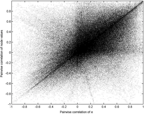
Finally it might be interesting to look whether the interbank market actually increases cor-relations between banks or whether it allows banks to diversify risk which reduces correlation. Remember that in our model, we describe the banking system by separately considering inter-bank business and all other inter-bank activities. In Figure 5 we look at the pairwise correlations across scenarios of bank values generated by all activities apart from interbank business (the vectore) and plot them against the pairwise correlations of bank values once we take the in-terbank part (after clearing) into account. Inin-terbank relations can in principle lead to lower or higher correlations or they may have no effect. No effect would imply that all values were clustered around the diagonal, a diversification effect of the interbank market would cause the correlations to be below the diagonal. We can see that the interbank market changes the pair-wise correlations of many bank values considerably, but there is no obvious trend. This picture thus gives further evidence that the network of mutual credit obligations has indeed an effect on the risk structure of the banking system.

7

Using the Model as an Experimentation Tool

While our model’s main focus is an integrated risk analysis for a banking system it can of course also be used in the traditional way of the previous contagion literature discussed in the beginning. This use basically consists of thought experiments that try to figure out the consequences of certain hypothetical events like the idiosyncratic failure of a big institution. In the following we want to demonstrate some such exercises with our model and the Austrian data. This will also give us the opportunity to further discuss the relation of our study to previous results on systemic risk and contagion of default.

In our first thought experiment we consider the possibility that bank insolvencies actually destroy some fraction of total assets. Note that the analysis so far, ignored this possibility. The clearing procedure distributed the entire value of an insolvent institution proportionally among the creditor banks. In the context of our model, the assumption of zero losses makes sense because the model just tries to assess technical insolvency of institutions that is implied by the data and the risk analysis. It is not a model that predicts bankruptcies. Still it might be interesting to ask, what would be the consequences if the technical insolvencies actually turned out to be true bank breakdowns that destroy asset values. In line with James (1991) who found that realized losses in bank failures can be estimated at around10%of total assets we chose our range of loss rates from 0,10%,25% up to 40% of total assets as our estimate of bankruptcy costs. The results are shown in Table 6.

Figure 5. Correlation of bank values with (node values) and without interbank positions (e) across different scenarios.

Assuming loss rates different from zero percent has little consequences for the ’typical’ scenario. In77%of the scenarios there are no contagious defaults irrespective of the assumed bankruptcy costs. Yet for some scenarios the consequences can be fairly dramatic. The maxi-mum number of contagious defaults increases sharply once we assume loss rates different from zero. For instance at a loss rate of 10% of total assets, the maximum number of contagious defaults is413(45%of all banks) compared to46(5%) with a loss rate of0%. As we can see, low bankruptcy costs are crucial to systemic stability of the banking system.

Another important issue is the question of how much funds the regulator needs to avoid fundamental or contagious defaults in each and every scenario. Being slightly less ambitious it could also be interesting to calculate the funds needed for insolvency avoidance in90,95,99 percent of the scenarios very much in the spirit of a value at risk model. Our framework can be used for such estimations. As shown in Table 7, a complete avoidance strategy amounts to about 8.5 billion Euro, which corresponds to 1.5% of all the assets held by the banks in the system. By only focusing on avoiding fundamental defaults in 99% of the scenarios the regulator can decrease this amount to about1.7billion Euro (or 0.31% of all total assets). The