Systematicity in sentence processing with a
recursive self-organizing neural network
Igor Farkaˇs1 and Matthew W. Crocker2 1- Dept. of Aplied Informatics, Comenius University Mlynsk´a dolina, 842 48 Bratislava, Slovak Republic 2- Dept. of Computational Linguistics, Saarland University
Saarbr¨ucken, 66041, Germany
Abstract. As potential candidates for human cognition, connection-ist models of sentence processing must learn to behave systematically by generalizing from a small traning set. It was recently shown that Elman networks and, to a greater extent, echo state networks (ESN) possess lim-ited ability to generalize in artificial language learning tasks. We study this capacity for the recently introduced recursive self-organizing neural network model and show that its performance is comparable with ESNs.
1
Introduction
To be considered a viable approach to human cognition, connectionist models must be able to account for the systematicity in human language. This poten-tial capability was questioned by Fodor and Pylyshyn [1] and is still a matter of debate. Hadley [2] noted that systematicity is a matter of learning and gen-eralization, and made a distinction betweeen weak and strong systematicity. A network is weakly systematic if it can process sentences with novel combinations of words, but these words are in the syntactic positions they also occurred in dur-ing traindur-ing (e.g. the network trained on sentencesboy loves girlanddog chases cat can also processdog chases girl). Strong systematicity, on the other hand, does require generalization to new syntactic positions (e.g. ability to processdog chases boy, provided thatboynever appeared as object during training).
According to Hadley, connectionist models were at best weakly systematic. But van der Velde [3], using simulations with the Elman’s simple recurrent net-work (SRN) in a next-word prediction task, claimed that even weak systematicity lies beyond the abilities of connectionist models. However, Frank [4] extended these simulations and showed that even SRN showed some generalization perfor-mance whose limitations arose from overfitting in large networks. Furthermore, he demonstrated that generalization could be improved by employing an alter-native architecture – the echo-state network (ESN; [5]) that requires less training and does not suffer from overfitting.
We investigated the potential benefit of self-organization in learning context representations by experimenting with various recursive self-organizing modules, coupled with two types of a single-layer prediction module [6]. In a next-word prediction language task we showed that the best performance was achieved by the so called RecSOMsard module (explained below) coupled with a simple
perceptron. In this paper, we investigate the weak syntactic systematicity of the RecSOMsard-based model and compare the performance with ESN [4].
2
Input data
The sentences were constructed using the grammar in Table 1, which subsumes the grammar used in [3]. The language consists of three sentence types: sim-ple sentences with an N-V-N structure, and two types of comsim-plex sentences, namely, right-branching sentences with an N-V-N-who-V-N structure and
centre-embedded sentences with an N-who-N-V-V-N structure. Complex sentence types
represent commonly used English sentences such asboy loves girl who walks dog
andgirl who boy loves walks dog, respectively.
S→Simple (.2)|Right (.4)|Centre (.4) N→N1|N2|N3|N4
Simple→N V N . V→V1|V2|V3|V4
Right→N V NwhoV N . Nx→nx1|nx2|... Centre→NwhoN V V N . Vx→vx1|vx2|...
Table 1: Grammar used for generating training and test sentences. Content words (nouns and verbs) are divided into four groups N1, ...,N4and V1, ...,V4. IfW denotes the lexicon size (i.e. the total number of word types
in the language), each group has (W-2)/8 nouns and the same number of verbs
(whoand ”.” are also considered words). Hence, forW=18 we have four nouns
and four verbs per group. The training set consisted of all sentences in which all content words were taken from the same group, i.e. simple sentences had the form ”nxivxj nxk .” (analogically for complex sentences). The range of indicesi, j, k
depends on W. In contrast to training sentences, each test sentence contained content words from as many different groups as possible (as the most complicated case, pursued in [3, 4]), i.e. each simple sentence had the form ”nxi vyj nzk .”, where x=y=z. This training scheme ensured that the proportion of training sentences relative to all possible sentences remained very small (∼0.4%).
3
RecSOMsard-P2 model
Our model consists of two modules that can be trained separately: a context-learning RecSOMsard and a two-layer perceptron (P2). Adding a hidden layer of units in the prediction module was shown to enhance prediction accuracy [4] and hence is used also here for consistency.
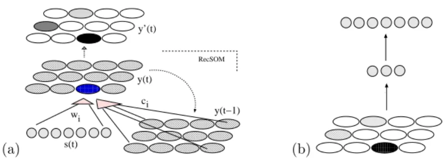
The architecture of the RecSOMsard module is shown in Figure 1a. It is based on RecSOM that has an extra top layer attached to it. Each RecSOM unit
i∈ {1,2, ..., N}has two weight vectors associated with it: wi∈ RW linked with anW-dimensional inputs(t), andci ∈ RN linked with the context y(t−1) = (y1(t−1), y2(t−1), ..., yN(t−1)).
The output of a unitiat time tis computed as yi(t) = exp(−di(t)), where
(a) 000000 000000 000000 000000 111111 111111 111111 111111 000000 000000 000000 000000 111111 111111 111111 111111 0000000 0000000 0000000 0000000 1111111 1111111 1111111 1111111 0000000 0000000 0000000 1111111 1111111 1111111 000000 000000 000000 111111 111111 111111 000000 000000 000000 111111 111111 111111 0000000 0000000 0000000 1111111 1111111 1111111 000000 000000 000000 111111 111111 111111 000000 000000 000000 000000 111111 111111 111111 111111 0000000 0000000 0000000 1111111 1111111 1111111 000000 000000 000000 111111 111111 111111 000000 000000 000000 000000 111111 111111 111111 111111 000000 000000 000000 000000 111111 111111 111111 111111 000000 000000 000000 000000 111111 111111 111111 111111 0000000 0000000 0000000 0000000 1111111 1111111 1111111 1111111 0000000 0000000 0000000 1111111 1111111 1111111 000000 000000 000000 111111 111111 111111 0000000 0000000 0000000 0000000 1111111 1111111 1111111 1111111 000000 000000 000000 111111 111111 111111 000000 000000 000000 000000 111111 111111 111111 111111 000000 000000 000000 000000 111111 111111 111111 111111 000000 000000 000000 111111 111111 111111 0000000 0000000 0000000 0000000 1111111 1111111 1111111 1111111 0000000 0000000 0000000 1111111 1111111 1111111 y(t) wi s(t) ci y(t−1) y’(t) RecSOM (b) 00000000000000000000000000 0000000000000 1111111111111 1111111111111 1111111111111 000000 000000 000000 000000 000000 000000 111111 111111 111111 111111 111111 111111
Fig. 1: (a) RecSOMsard architecture. The bottom part (without the top layer) represents RecSOM whose activity vectoryis transformed toy’ by a mechanism described in the text. (b) A two-layer perceptron with inputsy’.
Parameters α >0 and β >0 respectively influence the effect of the input and the context upon a unit’s profile. Both weight vectors can be updated using the same form of rule: Δwi=γhik(t)(s(t)−wi),and Δci=γhik(t)(y(t−1)−ci),
where k is an index of the winner (i.e. the unit with the highest yk(t)), and
0<γ<1 is the learning rate [7]. Radius of the neighborhood function hik(t)
lin-early decreases in time to allow for forming topographic representation of input sequences. RecSOM units self-organize to topographically represent temporal contexts (subsequences) in a Markovian manner. At the same time, a more complex sequence can lead to non-Markovian behavior [8]. For an overview of recursive self-organizing networks see [10].
The RecSOMsard module contains a SardNet-like [9] output postprocessing to be fed to a prediction module. In each iteration, the winner’s activation
yi in RecSOM is transformed to a sharp Gaussian profile yi centered arround
the winner, and previous activations in the top layer are decayed via y←λy
(as in SardNet). At boundaries between sequences, all yi are reset to zero.
This transforms the activation vector y(t) with mostly unimodal shape into a distributed activation vectory(t) whose number of peaks equals the position of a current word in a sentence. This way, the context in RecSOMsard becomes represented both spatially (due to SardNet) and temporally (due to RecSOM). Training the networks. Using localist encodings of words, networks were trained on the next word prediction task (i.e. one word at a time). All training sentences were concatenated in random order. The ratio of complex to simple sentences was 4:1. For each model and lexicon size, 10 networks were trained for
∼300,000 iterations and differed only in initial weights, randomly set to small
values. Some RecSOMsard parameters were fixed: λ=0.9, γ=0.1, the effect of
others was investigated (N, α, β). The perceptron, having 10 hidden units with logistic activation function (as in [4]), was trained by online back-propagation (without momentum), with learning rate set to linearly decrease from 0.1 to 0.01. Cross-entropy was used as an error function, therefore the perceptron output units had softmax activation functions, i.e. ai= eneti/jenetj, where
18 26 34 42 0.0 0.1 0.2 0.3 simple GPE 18 26 34 42 0.0 0.1 0.2 0.3 right−branching 18 26 34 42 0.0 0.1 0.2 0.3 centre−embedded
Fig. 2: Mean GPE measure for the three sentence types as a function of lexicon size W. Error bars were negligible for training data denoted by ’x’ and hence are not shown. The lines marked with ’o’ refer to the testing data.
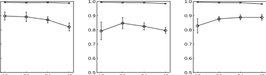
18 26 34 42 0.5 0.6 0.7 0.8 0.9 1.0 simple FGP 18 26 34 42 0.5 0.6 0.7 0.8 0.9 1.0 right−branching 18 26 34 42 0.5 0.6 0.7 0.8 0.9 1.0 centre−embedded
Fig. 3: Mean FGP measure for the three sentence types as a function of lexicon sizeW (’x’ = training data, ’o’ = testing data).
4
Results
We rated the network performance using two measures. One is the grammatical prediction error (GPE) defined as the ratio of the sum of non-grammatical output activations a(¬G) =i/∈Gai and the sum of total output activation a(¬G) +
a(G) [3]. Since we have softmax output units, GPE = a(¬G). Frank argues
that GPE lacks the baseline (that would correspond to the network with no generalization) and that this problem is overcome in the alternative measure he introduced (see [4] for details) to quantify the generalization (we will call it Frank’s generalization performance, FGP). FGP is based on comparing network’s
a(G) with the predictionsb(G) of a bigram statistical model. The marginal cases result as follows: Ifa(G) = 1, then FGP = 1 (perfect generalization); ifa(G) = 0 (completely non-grammatical predictions), then FGP = -1; a non-generalizing network with a(G) = b(G) (i.e. behaving as a bigram model) would yield FGP = 0. Hence, positive FGP score measures degree of generalization.
We ran extensive simulations that can be divided into three stages:
(1) Effect of N: We looked for a reasonable number of map units N (using
map radii 9, 10, 12, 14, 16) and found that beyond N = 12×12 = 144 the
test performance stopped to significantly improve. Hence, for all subsequent simulations we used this network size.
(2)Effect ofαandβ: We found that the mean GPE (e.g. its slope as a function
of W) depended on specific values of map parameters. At the same time, we
found the following conditions resulting in best performance: 0.8≤α≤1.5, 0.2≤β≤0.6 and 0.4≤α−β≤1.1. Figure 2 shows the mean of mean GPEs (computed for 8 concreteα-β pairs from the above intervals) as a function ofW. Training error was negligible, and test error that remains below 10% can be seen to reduce with larger lexicon. Similar dependence was observed in [4] in terms of increasing FGP, both in case of SRN and ESN models. In our model (Figure 3), in terms of FGP this trend is only visible for centre-embedded sentences. Also, our FGP values are a little bit worse than those of ESN [4], but still clearly indicating the presence of generalization.
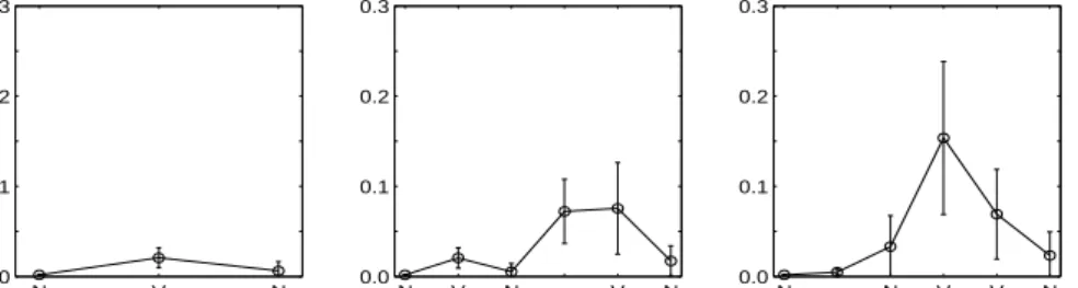
N V N 0.0 0.1 0.2 0.3 GPE simple N V N w V N 0.0 0.1 0.2 0.3 right−branching N w N V V N 0.0 0.1 0.2 0.3 centre−embedded
Fig. 4: Mean GPE for the three sentence types, averaged over test sentences and all lexicon sizes (N= 144, α= 0.8, β= 0.4).
N V N 0.5 0.6 0.7 0.8 0.9 1.0 FGP simple N V N w V N 0.5 0.6 0.7 0.8 0.9 1.0 right−branching N w N V V N 0.5 0.6 0.7 0.8 0.9 1.0 centre−embedded
Fig. 5: Mean FGP for the three sentence types, averaged over test sentences and all lexicon sizes (N= 144, α= 0.8, β= 0.4).
(3) Mean word predictions: Next, we took the model (given by N, α, β) with the lowest mean GPE and calculated its performance for individual inputs (words) in tested sentences, averaged over all lexicon sizes (N). Again, GPE on training data was close to 0. Results for test data are shown in Figure 4. The corresponding performance in terms of FGP in Figure 5 stays above 0.6.
Compared to ESN [4], this falls between the best ESN model (for bestW and
N) whose FGP≥0.8 and the mean FGP performance (averaged overW andN)
which drops to 0.5 for most difficult cases in complex sentences. In our model, the most difficult predictions were similar for all word positions, and can be seen
from both figures. Unlike ESN, end-of-sentence markers were predicted very well by our model. Both figures suggest that the RecSOMsard-P2 network is also capable of generalization. The two measures appear to be inversely related, but differ in the fact that only FGP depends on bigram performance (which could explain different peak positions in the two graphs for complex sentences with centre-embedding).
5
Conclusion
In the context of weak systematicity, we showed that RecSOMsard-P2, like ESN, considerably avoids making non-grammatical predictions (quantified by GPE measure), and by doing that, it displays some generalization (quantified by pos-itive FGP). A more rigorous comparison study with more complex data would be required in order to find out to what extent self-organization has its merits in learning context representations, as opposed to untrained weights used in ESN. This type of work aims to shed light on the question how purely unbiased, dis-tributional information can inform the learning the systematic syntactic knowl-edge in a variety of neural net architectures and training scenarios (SRN, ESN, RecSOMsard). This observation undermines the claim made by Fodor and Py-lylshyn (or some of their supporters) that even if you find one example of con-nectionist systematicity, it doesn’t really count because connectionism should be systematic “in general” to be taken seriously as a cognitive model. Investigat-ing this learnInvestigat-ing ability is a prerequisite to developInvestigat-ing more cognitively faithful models, such as of infant language acquisition.
Acknowledgment: The core of this work was done while I. F. was at Saarland University sponsored by the Humboldt Foundation. He was also supported by Slovak Grant Agency for Science. Thanks to Stefan Frank for fruitful comments.
References
[1] J.A. Fodor and Z.W. Pylyshyn. Connectionism and cognitive architecture: A critical analysis. Cognition, 28:3–71, 1988.
[2] R.F. Hadley. Systematicity in connectionist language learning. Mind and Language, 9(3):247–272, 1994.
[3] F. van der Velde, G. van der Voort van der Kleij, and M. de Kamps. Lack of combinatorial productivity in language processing with simple recurrent networks. Connection Science, 16(1):21–46, 2004.
[4] S. Frank. Learn more by training less: systematicity in sentence processing by recurrent networks. Connection Science, 18(3):287–302, 2006.
[5] H. Jaeger. Adaptive nonlinear system identification with echo state networks. InAdvances in NIPS, 15, pp. 593–600, MIT Press, 2003.
[6] I. Farkaˇs and M.W. Crocker. Recurrent networks and natural language: exploiting self-organization. InProc. of 28th Ann. Conf. of Cog. Sci. Soc., pp. 1275–1280, 2006. [7] T. Voegtlin. Recursive self-organizing maps. Neural Networks, 15(8-9):979–992, 2002. [8] P. Tiˇno, I. Farkaˇs, and J. van Mourik. Dynamics and topographic organization in recursive
self-organizing map. Neural Computation, 18:2529–2567, 2006.
[9] D. James and R. Miikkulainen. SardNet: a self-organizing feature map for sequences. In
Advances in NIPS, 7,pp. 577–584. MIT Press, 1995.
[10] B. Hammer, A. Micheli, A. Sperduti and M. Strickert. Recursive self-organizing network models. Neural Networks, 17:1061–1085, 2004.