Corporate Policies with
Temporary and Permanent Shocks
∗
J.-P. D´
ecamps
†S. Gryglewicz
‡E. Morellec
§S. Villeneuve
¶September 16, 2015
Abstract
We develop a dynamic model of investment, financing, liquidity and risk manage-ment policies in which firms face financing frictions and are subject to permanent and temporary cash flow shocks. In this model, more profitable firms access equity mar-kets less often but raise more funds when doing so. The cash-flow sensitivity of cash increases with financing constraints and cash flow volatility. Persistence of cash flow shocks and volatility of permanent shocks help manage corporate liquidity. Tempo-rary shocks volatility hinders it. Hedging permanent or tempoTempo-rary shocks may involve opposite positions. Derivatives usage and asset substitution are not equivalent when hedging permanent shocks.
Keywords: Corporate policies; permanent vs. temporary shocks; financing frictions. JEL Classification Numbers: G31, G32, G35.
∗We have received helpful comments from Sudipto Dasgupta, Hae Won Jung, Andrey Malenko (EFA
discusant) Jean-Charles Rochet, as well as seminar participants at the University of Lancaster, the University of Zurich, the 2015 Finance Down Under conference, and the 2015 EFA meetings. Jean-Paul D´ecamps and St´ephane Villeneuve acknowledge financial support of the SCOR research initiative Market Risk and Creation Value. Erwan Morellec acknowledges financial support from the Swiss Finance Institute.
†Toulouse School of Economics. ‡Erasmus University Rotterdam.
§Swiss Finance Institute, EPFL, and CEPR. ¶Toulouse School of Economics.
During the past two decades, dynamic corporate finance models have become part of the mainstream literature in financial economics, providing insights and quantitative guidance for investment, financing, cash management, or risk management decisions under uncertainty. Two popular cash flow environments have been used extensively in this literature. In one, shocks are of permanent nature and cash flows are governed by a geometric Brownian motion (i.e. their growth rate is normally distributed). This environment has been a cornerstone of dynamic capital structure models (see e.g. Leland (1998) or Strebulaev (2007)) and real-options models (see e.g. McDonald and Siegel (1986) or Morellec and Sch¨urhoff (2011)). In the other, shocks are of temporary nature and short-term cash flows are modeled by the increments of an arithmetic Brownian motion (i.e. cash flows are normally distributed). This has proved useful in models of liquidity management (see e.g. D´ecamps, Mariotti, Rochet, and Villeneuve (2011) or Bolton, Chen, and Wang (2011)) and in models of dynamic agency (see e.g. DeMarzo and Sannikov (2006) or Biais, Mariotti, Plantin, and Rochet (2007)).1
Assuming that shocks are either of permanent or temporary nature has the effect of dra-matically simplifying dynamic models. However, corporate cash flows cannot generally be fully described using solely temporary or permanent shocks. Many types of production, mar-ket, or macroeconomic shocks are of temporary nature and do not affect long-term prospects. But long-term cash flows also change over time due to various firm, industry, or macroeco-nomic shocks that are of permanent nature. In addition, focusing on one type of shocks produces implications that are sometimes inconsistent with the evidence. For example, in models based solely on permanent shocks, cash flows cannot be negative without having negative asset values, the volatilities of earnings and asset value growth rates are equal, and innovations in cash flows are perfectly correlated with those in asset values (see Gorbenko and Strebulaev (2010)). In liquidity management models based solely on temporary shocks, cash holdings are the only state variable for the firm’s problem, equity issues always have the same size, and the cash-flow sensitivity of cash is either zero or one.
1See Strebulaev and Whited (2012) for a recent survey of models based on permanent shocks. See
Moreno-Bromberg and Rochet (2014) for a recent survey of liquidity models based on temporary shocks. See Biais, Mariotti, and Rochet (2013) for a recent survey of dynamic contracting models.
Our objective in this paper is therefore twofold. First, we seek to develop a dynamic model of investment, financing, cash holdings, and risk management decisions in which firms are exposed to both permanent and temporary cash flow shocks. Second, we want to use this model to shed light on existing empirical results and generate novel testable implications.
A prerequisite for our study is a model that captures in a simple fashion the joint effects of permanent and temporary shocks on firms’ policy choices. In this paper, we base our analysis on a model of cash holdings and financing decisions with financing frictions in the spirit of D´ecamps, Mariotti, Rochet, and Villeneuve (2011), to which we add permanent shocks, an initial investment decision, and an analysis of risk management policies.
Specifically, we consider a firm with a valuable real investment opportunity. To undertake the investment project, the firm needs to raise costly outside funds. The firm has full flexibility in the timing of investment but the decision to invest is irreversible. The investment project, once completed, produces a stochastic stream of cash flows that depend on both permanent and temporary shocks. To account for the fundamentally different nature of these shocks, we model the firm cash flows in the following way. First, cash flows are subject to profitability shocks that are permanent in nature and governed by a geometric Brownian motion, as in standard real options and dynamic capital structure models. Second, for any given level of profitability, cash flows are also subject to short-term shocks that expose the firm to potential losses. These short-term cash flow shocks may be of temporary nature but they may also be correlated with permanent shocks, reflecting the level of cash flow persistence. In the model, the losses due to short-term shocks can be covered either using cash holdings or by raising funds at a cost in the capital markets. The firm may also hedge its exposure to permanent and temporary shocks by investing in financial derivatives or by changing its exposure to these shocks (via asset substitution). When making investment, liquidity, financing, and hedging decisions, management maximizes shareholder value.
Using this model, we generate two sorts of implications. First, we show that a combina-tion of temporary and permanent shocks can lead to policy choices that are in stark contrast with those in models based on a single source of risk. Second, our analysis demonstrates
that temporary and permanent risks have different, often opposing, implications for corpo-rate policies. Combining them produces implications that are consistent with a number of stylized facts and allows us to generate a rich set of testable predictions.
We highlight the main empirical implications. In standard real options models in which firms are solely exposed to permanent shocks and face financing frictions when seeking to invest in new projects, future financing constraints feed back in current policy choices by encouraging early investment (see for example Boyle and Guthrie (2003)). In contrast, we find that the combination of financing frictions and temporary shocks delays investment. This delay is due to two separate effects. First, the cost of external finance increases the cost of investment, making the investment opportunity less attractive and leading to an increase in the profitability level required for investment. Second, the combination of temporary shocks and financing frictions reduces the value of the firm after investment, further delaying investment. That is, the threat of future cash shortfalls increases future financing costs and reduces the value of the asset underlying the growth option, thereby leading to late exercise of the investment opportunity. We also show that the effect can be quantitatively important. In our base case environment for example, investment is triggered for a profitability level that is 10% higher than in models without temporary shocks and financing frictions.2
After investment, the value of a constrained firm depends not only on the level of its cash reserves, as in prior dynamic models with financing frictions, but also on the value of the permanent shock (i.e. profitability). Notably, one interesting and unique feature of our model is that the ratio of cash holdings over profitability is the state variable of the firm’s problem. This is largely consistent with the approach taken in the empirical literature (see for example Opler, Pinkowitz, Stulz, and Williamson (1999)), but it has not been clearly motivated by theory. Given that the empirical literature uses a related proxy, it may not seem a very notable observation that cash holdings are scaled by profitability. However,
2See for example the early papers of McDonald and Siegel (1986) and Dixit (1989) or the recent
contribu-tions of Carlson, Fisher, and Giammarino (2004), Lambrecht (2004), Manso (2008), Grenadier and Malenko (2010), Carlson, Fisher, and Giammarino (2010), or Grenadier and Malenko (2011). Dixit and Pindyck (1994) and Stokey (2009) provide excellent surveys of this literature.
the observation that “effective cash = cash/profitability” implies that more profitable firms hold more cash. That is, as the long-term prospects of the firm improve following positive permanent shocks, the firm becomes more valuable and finds it optimal to hoard more cash. By contrast, negative permanent shocks decrease firm value and, consequently, the optimal level of precautionary cash reserves.
We show in the paper that this relation between permanent shocks and target cash holdings has numerous implications. First, a standard result in corporate-liquidity models based solely on temporary shocks is that the cash-flow sensitivity of cash is either zero (at the target level of cash reserves ) or one (away from the target). In contrast, our model predicts that firms demonstrate a non-trivial and realistic cash-flow sensitivity of cash, due to the effects of permanent shocks on target cash holdings. In our model, this sensitivity is measured by an explicit expression that depends on a number of firm, industry, or market characteristics. In particular, this sensitivity increases with financing frictions, consistent with the evidence in Almeida, Campello, and Weisbach (2004). Second, the relation between permanent shocks and target cash holdings implies that when firms access capital markets to raise funds, the size of equity issues is not constant as in prior studies, but depends on the firm’s profitability. Notably, a unique prediction of our model is that more profitable firms raise more funds when accessing financial markets.
A third key implication of the relation between permanent shocks and target cash holdings concerns the effects of risk and uncertainty on cash holdings and firm value. We show in the paper that firm value increases in correlation between short-term and permanent shocks, that is, in the persistence of cash flow shocks. This is not immediately expected because two correlated shocks of temporary nature would allow for diversification if correlation decreased. So firm value would decrease in correlation between temporary shocks. Intuitively, the firm benefits from increased correlation between short-term and permanent shocks because it is then able to generate cash flows when they are needed to maintain scaled cash holdings after positive permanent shocks. Another related implication is that an increase in the volatility of permanent cash flow shocks can increase firm value as long as permanent shocks
are correlated with temporary shocks. This effect arises despite the concavity of the value function and is due to the fact that volatility in permanent cash flow shocks can help manage liquidity when short-term shocks display persistence.
Similar intuition applies to our predictions on cash holdings. Notably, target cash hold-ings decrease with the persistence of cash flow shocks and can decrease with the volatility of permanent shocks if persistence is positive. Importantly, we also find that permanent shocks have large quantitative effects on firm value and optimal policies. Using conservative parameter values, the inclusion of permanent shocks in the model increases firm value by 19% and decreases target cash holdings by 12%.
Turning to risk management, we show that derivatives usage should depend on whether the risk stems from temporary or permanent shocks. Specifically, if futures prices and the firm’s risk are positively correlated, then hedging temporary shocks involves a short futures position while hedging permanent shocks may involve a long futures position. (And vice versa if the correlation is negative.) This means that hedging permanent shocks may take a position not contrary but aligned to exposure. In these instances, the firm prefers to increase cash flow volatility to increase cash flow correlation to permanent profitability shocks.
We also show that managing risk either by derivatives or by directly selecting the riskiness of assets (i.e. asset substitution) leads to the same outcome if the risk is due to temporary shocks. However, hedging with derivatives and asset substitution are not equivalent when managing the risk from permanent shocks. This is due to the fact that asset substitution does not generate immediate cash flows whereas derivatives do. This may not matter for an unconstrained firm, but it is a fundamental difference for a financially constrained firm. One prediction of the model is thus that a firm in distress would engage asset substitution with respect to permanent shocks but not in derivatives hedging. Lastly, when risk management is costly, constrained firms hedge less, consistent with the evidence in Rampini, Sufi, and Viswanathan (2014) that collateral constraints pay a major role in risk management. Again, these predictions are very different from those in models based on a single source of risk (see e.g. Bolton, Chen, and Wang (2011) or Hugonnier, Malamud, and Morellec (2015)).
As relevant as it is to analyze an integrated framework combining both temporary and permanent shocks, there are surprisingly only a few attempts in the literature addressing this problem. Gorbenko and Strebulaev (2010) consider a dynamic model without financing frictions, in which firm cash flows are subject to both permanent and temporary shocks. Their study focuses leverage choices. Our paper instead analyzes liquidity, refinancing, risk management, and investment policies. Another important difference between the two papers is that we model temporary shocks with a Brownian process instead of a Poisson process. Grenadier and Malenko (2010) build a real options model in which firms are uncertain about the permanence of past shocks and have the option to learn before investing. In their model, there are no financing frictions and, as a result, no role for cash holdings and no need to optimize financing decisions.
Our work is also directly related to the recent papers that incorporate financing frictions into dynamic models of corporate financial decisions. These include Bolton, Chen, and Wang (2011), D´ecamps, Mariotti, Rochet, and Villeneuve (2011), Gryglewicz (2011), Bolton, Chen, and Wang (2013), and Hugonnier, Malamud, and Morellec (2015). A key simplifying assumption in this literature is that cash flows are only subject to transitory shocks. That is, none of these papers has permanent shocks together with temporary shocks. As we show in this paper, incorporating permanent shocks in models with financing frictions leads to a richer set of empirical predictions and helps explain corporate behavior.3
The paper is organized as follows. Section 1 describes the model. Section 2 solves for the value of a financially constrained firm and for the real option to invest in this firm. Section 3 derives the model’s empirical implications. Section 4 examines risk management policies. Section 5 concludes. Technical developments are gathered in the Appendix.
3In a recent empirical study, Chang, Dasgupta, Wong, and Yao (2014) show that decomposing corporate
cash flows into a transitory and a permanent component helps better understand how firms allocate cash flows and whether financial constraints matter in this allocation decision.
1
Model
1.1
Assumptions
Throughout the paper, agents are risk neutral and discount cash flows at a constant rate
r > 0. Time is continuous and uncertainty is modeled by a probability space (Ω,F,F, P) with the filtrationF={Ft:t≥0}, satisfying the usual conditions.
We consider a firm that owns an option to invest in a risky project. The firm has full flexibility in the timing of investment but the decision to invest is irreversible. The direct cost of investment is constant, denoted by I >0. The project, once completed, produces a continuous stream of cash flows that are subject to both permanent and temporary shocks. Permanent shocks change the long-term prospects of the firm and influence cash flows per-manently by affecting the productivity of assets (and firm size). We denote the productivity of assets byA = (At)t≥0 and assume that it is governed by a geometric Brownian motion:
dAt =µAtdt+σAAtdWtP, (1)
where µ and σA > 0 are constant parameters and WP = (WtP)t≥0 is a standard Brownian motion. In addition to these permanent shocks, cash flows are subject to short-term shocks that do not necessarily affect long-term prospects. Notably, we consider that operating cash flows dXt after investment are proportional to At but uncertain and governed by:
dXt=αAtdt+σXAtdWtX, (2)
where α and σX are strictly positive constants and WX = (WtX)t≥0 is a standard Brownian motion. WX is allowed to be correlated with WP with correlation coefficient ρ, in that
E[dWtPdW X
t ] =ρdt. (3)
The dynamics of cash flows can then be rewritten as
dXt=αAtdt+σXAt(ρdWtP + p
1−ρ2dWT
where WT = (WT
t )t≥0 is a Brownian motion independent from WP. This decomposition implies that short-term cash flow shocks dWX
t consist of temporary shocksdWtT and
persis-tent shocks dWtP and that ρ is a measure of persistence of short-term cash flow shocks.4 In what follows we refer to σX as the volatility of short-term shocks or, when it does not cause
confusion, as the volatility of temporary cash flow shocks.
The permanent nature of innovations in A implies that a unit increase or decrease in A
increases or decreases the expected value of each future cash flow. To illustrate this property, it is useful to consider an environment in which the firm has a frictionless access to capital markets, as in e.g. Leland (1994) or McDonald and Siegel (1986). In this case, the value of the firm after investment VF B is simply given by the present value of all future cash flows
produced by the firm’s assets. That is, we have
VF B(a) =Ea Z ∞ 0 e−rtdXt = αa r−µ. (5)
Equation (5) shows that a shock that changes At via dWtP is permanent in the sense that
a unit increase in At will increase all future expected levels of profitability by that unit
(adjusted for the drift). A shock to WT
t is temporary because, keeping everything else
constant, it has no impact on future cash flows. That is, when cash flow shocks are not persistent, i.e. when ρ = 0, short-term cash flow shocks do not affect future level of cash flows. When cash flows shock are perfectly persistent, i.e. when ρ= 1, any cash flow shocks impact all future cash flows. Realistically, cash flow shocks are persistent but not perfectly and ρ is expected to take values between 0 and 1 for most firms.
The modeling of cash flows in equations (1) and (2) encompasses two popular frameworks as special cases. Ifµ=σA= 0, we obtain the stationary framework of the models of liquidity
management (see D´ecamps, Mariotti, Rochet, and Villeneuve (2011), Bolton, Chen, and Wang (2011), Hugonnier, Malamud, and Morellec (2015)) and dynamic agency (see DeMarzo
4One may also interpretWT as a shock to cash flow and WP as a shock to asset value. In our model,
a pure cash flow shock (cash windfall) makes the firm richer but does not make the firm’s assets better. A pure shock to assets (e.g., discovery of oil reserves) improves the value of the firm’s assets does not make the firm richer today. We thank Andrey Malenko for suggesting this interpretation.
and Sannikov (2006) or DeMarzo, Fishman, He, and Wang (2012)). As we show below, adding permanent shocks in these models gives rise to two sources of dynamic uncertainty that makes corporate policies intrinsically richer. IfσX = 0, we obtain the model with
time-varying profitability applied extensively in dynamic capital structure models (see Goldstein, Ju, and Leland (2001), Hackbarth, Miao, and Morellec (2006), Strebulaev (2007)) and real-options analysis (see Dixit and Pindyck (1994), Carlson, Fisher, and Giammarino (2006), Morellec and Sch¨urhoff (2011)). Our model with temporary and permanent shocks differs from the latter in that earnings and asset volatilities differ and innovations in current cash flows are imperfectly correlated with those in asset values. As discussed in Gorbenko and Strebulaev (2010), these features are consistent with empirical stylized facts.
1.2
Shareholders’ optimization problem
In the absence of short-term shocks, the cash flows of an active firm are always positive becauseA is always positive. The short-term shockWX exposes the firm to potential losses,
that can be covered either using cash reserves or by raising outside funds. Specifically, we allow management to retain earnings inside the firm and denote by Mt the firm’s cash
holdings at any time t > 0. These cash reserves earn a constant interest rate r−λ inside the firm, where λ∈(0, r] is a cost of holding liquidity.
We also allow the firm to increase its cash holdings or cover operating losses by raising funds in the capital markets. When raising outside funds at time t, the firm has to pay a proportional cost p >1 and a fixed cost φAt so that if the firm raises some amount et from
investors, it gets et/p−φAt. As in Bolton, Chen, and Wang (2011), the fixed cost scales
with firm size so that the firm does not grow out from the fixed cost.5 The net proceeds
5The scaling of the fixed refinancing cost can be motivated by modeling the origins of this cost as in
Hugonnier, Malamud, and Morellec (2015). Suppose that new investors have some bargaining power in the division of the surplus created at refinancing. A Nash-bargaining solution would allocate a share of this surplus to new investors. As it becomes clear below in Section 2.1, the total surplus at refinancing is linear in profitabilityAt. This approach would generate a fixed refinancing costφAtwith an endogenousφ.
from equity issues are then stored in the cash reserve, whose dynamics evolve as:
dMt= (r−λ)Mtdt+dXt+
dEt
p −dΦt−dLt, (6)
whereLt,Et, and Φtare non-decreasing processes that respectively represent the cumulative
dividend paid to shareholders, the cumulative gross external financing raised from outside investors, and the cumulative fixed cost of financing.
Equation (6) is an accounting identity that indicates that cash reserves increase with the interest earned on cash holdings (first term on the right hand side), the firm’s earnings (second term), and outside financing (third term), and decrease with financing costs (fourth term) and dividend payments (last term). In this equation, the cumulative gross financing raised from investors Et and the cumulative fixed cost of financing Φt are defined as:
Φt= ∞ X n=1 φAτn1τn≤t and Et = ∞ X n=1 en1τn≤t,
for some increasing sequence of stopping times (τn)∞n=1 that represent the dates at which the firm raises funds from outside investors and some sequence of nonnegative random variables (en)∞n=1 that represent the gross financing amounts.6
The firm can abandon its assets at any time after investment by distributing all of its cash to shareholders. Alternatively, it can be liquidated if its cash buffer reaches zero following a series of negative shocks and raising outside funds to cover the shortfall is too costly. We consider that the liquidation value of assets represents a fraction ω <1 of their unconstrained valueVF B(a) plus current cash holdings. The liquidation time is then defined
byτ0 ≡ {t≥0|Mt= 0}. If τ0 =∞, the firm never chooses to liquidate.
Objective function. We solve the model backwards, starting with the value and optimal policies of an active firm. In a second stage, we derive the value-maximizing investment
6Technically, ((τ
n)n≥1,(en)n≥1, L) belongs to the setAof admissible policies if and only if (τn)n≥1 is a
non-decreasing sequence ofF-adapted stopping times, (en)n≥1is a sequence of nonnegative (Fτn)n≥1-adapted
policy for the firm’s growth option together with the value of the growth option.7
The objective of management after investment is choose the dividend, financing, and de-fault policies that maximize shareholder value. (We also analyze risk management in section 4.) There are two state variables for shareholders’ optimization problem after investment: Profitability At and the cash balance Mt. We can thus write shareholders’ problem as:
V(a, m) = sup (τn)n≥0,(en)n≥1,L Ea,m Z τ0 0 e−rt(dLt−dEt) +e−rτ0 ωαAτ0 r−µ +Mτ0 . (7)
The first term on the right hand side of equation (7) represents the present value of payments to incumbent shareholders until the liquidation timeτ0, net of the claim of new investors on future cash flows. The second term represents the firm’s discounted liquidation value.
Consider next shareholders’ investment decision. As discussed above, in the presence of temporary shocks and financing frictions, the firm will find it optimal to hold cash after investment. Thus, solving shareholders’ investment problem entails finding both the optimal time to invest as well as the value-maximizing initial level of cash reserves m0. Denote the value of the investment opportunity by G(a). Shareholders’ optimization problem before investment can be formally written as:
G(a) = sup τ,m0≥0 Ea e−rτ(V(Aτ, m0)−p(I+m0+φAτ)) . (8)
It is important to note that the realizations of temporary shocks do not matter before investment since they have no impact on the profitability of investment. That is, short-term shocks matter only in as much as they relate to long-short-term productivity. Therefore, the only state variable in the investment problem is the productivity of the asset underlying the project, a. However, the parameters governing the temporary shocks, σT, α, and ρ, do
influence the value of the investment opportunity and the optimal investment decision via their impact on the post-investment value of the firm.
7Our model can be extended to incorporate investment after entry, for example by allowing the firm to
affect the growth rateµof the profitability processAtvia costly investment in R&D or technology. Extending
2
Model solution
2.1
Value of an active firm
In this section, we base our analysis of shareholders’ problem (7) on heuristic arguments. These arguments are formalized in the Appendix. To solve problem (7) and find the value of an active firm, we need to determine the financing, payout, and liquidation policies that maximize shareholder value after investment. Consider first financing and liquidation deci-sions. Because of the fixed cost of financing, it is natural to conjecture that it is optimal for shareholders to delay equity issues as much as possible. That is, if any issuance activity takes place, this must be when cash holdings drop down to zero, so as to avoid liquidation. At this point, the firm will either issue shares if the fixed cost of financing is not too high or it will liquidate. Consider next payout decisions. In the model, cash reserves allow the firm to reduce refinancing costs or the risk of inefficient liquidation. As a result, the benefit of an additional dollar retained in the firm is decreasing in the firm’s cash reserves. Since keeping cash inside the firm entails an opportunity costλon any dollar saved, we conjecture that the optimal payout policy is characterized by a profitability-dependent target cash level m∗(a), such that all earnings are retained when the firm’s cash balance is below this level and all earnings are paid out when the cash balance is above this level.
To solve for firm value after investment, we first consider the region (0, m∗(a)) over which it is optimal to retain earnings. In this region, the firm does not deliver any cash flow to shareholders and equity value satisfies:
rV(a, m) = µaVa(a, m) + (αa+ (r−λ)m)Vm(a, m) (9) +1 2a 2 σ2 AVaa(a, m) + 2ρσAσXVam(a, m) +σX2Vmm(a, m) .
whereVxdenote the first-order derivative of the functionV with respect toxandVxy denotes
the second-order partial derivative of V with respect to x and y. The left-hand side of this equation represents the required rate of return for investing in the firm’s equity. The
right-hand side is the expected change in equity value in the region where the firm retains earnings. The first two terms capture the effects of changes in profitability and cash savings on equity value. The last term captures the effects of volatility in cash flows and productivity. In our model with permanent and temporary shocks, changes in productivity affect not only the value of an active firm but also the value of cash reserves.
Equation (9) is solved subject to the following boundary conditions. First, when cash holdings exceed m∗(a), the firm places no premium on internal funds and it is optimal to make a lump sum payment m−m∗(a) to shareholders. As a result, we have
V(a, m) = V(a, m∗(a)) +m−m∗(a), (10)
for all m ≥ m∗(a). Substracting V(a, m∗(a)) from both sides of this equation, dividing by
m−m∗(a), and taking the limit asm tends tom∗(a) yields the condition
Vm(a, m∗(a)) = 1. (11)
AsV is assumed to beC2across the boundary functionm∗(a), condition (11) in turn implies
the high-contact condition (see Dumas (1992)):
Vmm(a, m∗(a)) = 0, (12)
that determines the location of the dividend boundary function.
When the fixed cost of external finance φ is not too large, the firm raises funds every time its cash buffer is depleted. In this case, the value-matching condition at zero is
V(a,0) =V(a, m(a))−p(m(a) +φa), (13)
so that the value of the shareholders’ claim when raising outside financing is equal to the continuation value (first term on the right-hand side) less issuance costs (second term). The
value-maximizing issue size m(a) is then determined by the first-order condition:
Vm(a, m(a)) = p, (14)
which ensures that the marginal cost of outside funds is equal to the marginal benefits of cash holdings at the post-issuance level of cash reserves. As shown by this equation, the size of equity issues is not constant as in previous contributions, but depends on the firm’s productivity. Lastly, when the fixed cost of financing makes an equity issue unattractive, liquidation is optimal at m= 0 and we have:
V(a,0) = ωαa
r−µ. (15)
While there are two state variables for shareholders’ optimization problem (9)-(15), this problem is homogeneous of degree one in a and m. We can thus write:
V(a, m) = aV(1, m/a)≡aF(c), (16)
where c ≡ m
a represents the scaled cash holdings of the firm and F(c) is the scaled value
function. Using this observation, the boundary conditions can be rewritten in terms of the scaled value function as a standard free boundary problem with only one state variable, the scaled cash holdings of the firm that evolve between the liquidation/refinancing trigger located at zero and the payout trigger c∗. Anticipating, an application of Itˆo’s formula implies that the dynamics of scaled cash holdings is given by
dCt = α−σAσX +Ct(r−λ+µ+σA2) dt +σX p 1−ρ2dWT t +ρσXdWtP −CtσAdWtP + dEt p −dΦt−dLt.
This equation shows that a positive temporary shock (i.e. dWT
t >0) unambiguously brings
the firm closer to the target level of cash reserves c∗. A positive permanent shock has two opposing effects. First, for any given target level c∗, it moves the firm’s cash reserves closer
to c∗ (third term on the right hand side). Second, it makes assets more productive, leading to an increase in the demand for cash and to a greater distance between current cash reserves and the target level (fourth term).
We can now follow the same steps as above to derive shareholders’ modified (or scaled) optimization problem after investment.8 When scaled cash holdings are in (0, c∗), it is
optimal for shareholders to retain earnings and the scaled value function F(c) satisfies:
(r−µ)F(c) = (α+c(r−λ−µ))F0(c) + 1 2(σ 2 Ac 2−2ρσ AσXc+σX2)F 00 (c). (17)
At the payout trigger c∗, F(c) satisfies the value-matching and high-contact conditions
F0(c∗) = 1, (18)
F00(c∗) = 0. (19)
Additionally, when the firm runs out of cash, shareholders can either refinance or liquidate assets. As a result, the scaled value function satisfies
F(0) = max max c∈[−φ,∞)(F(c)−p(c+φ)) ; ωα r−µ . (20)
When refinancing at zero is optimal, scaled cash holdings after refinancing c are given by the solution to the first-order condition:
F0(c) = p. (21)
Lastly, in the payout regionc > c∗, the firm pays out any cash in excess of c∗ and we have
F(c) = F(c∗) +c−c∗. (22)
8Using equation (16), we have that V
m(a, m) = F0(c), Vmm(a, m) = 1aF00(c), Va(a, m) = F −cF0(c),
Vaa(a, m) = c
2
aF
00(c), and V
am(a, m) = −acF00(c). Plugging these expressions in the partial differential
Before solving shareholders’ problem, we can plug the value-matching and high-contact conditions (18)-(19) in equation (17) to determine the value of the firm at the target level of scaled cash holdings c∗. This shows that equity value satisfies
V(a, m∗(a)) = aF(c∗) = αa r−µ+ 1− λ r−µ m∗(a). (23)
Together with equation (5), equation (23) implies that equity value in a constrained firm holding m∗(a) units of cash is equal to the first best equity value minus the cost of holding liquidity, which is the product of the target level of cash holdings m∗(a) and the present value of the unit cost of holding cash r−λµ.
The following proposition summarizes these results and characterizes shareholders’ opti-mal policies and value function after investment.
Proposition 1. Consider a firm facing issuance costs of securities (φ >1, p >1), costs of carrying cash (0 < λ ≤ r), permanent shocks, and short-term shock that are not perfectly persistent (ρ <1). Then, the following holds:
1. The value of the firm, V(m, a) solving problem (7), satisfies the relation V(m, a) =
aF(ma), where (F, c∗) is the unique solution to the system (17)-(22).
2. The function F(c) is increasing and concave over (0,∞). F0(c) is strictly greater than one for c∈(0, c∗), where c∗ ≡inf{c >0|F0(c) = 1}, and equal to one for c∈[c∗,∞).
3. If issuance costs are high, it is never optimal to issue new shares after investment, F(0) = rωα−µ, and the firm is liquidated as soon as it runs out of cash.
4. If issuance costs are low,F(0) = maxc∈[−φ,∞)(F(c)−p(c+φ))> rωα−µ and it is optimal to raise a dollar amount e∗n =p(c+φ)Aτn from investors at each time τn at which the
firm runs out of cash, where c≡(F0)−1(p).
5. Whenm∈(0, m∗(a)), the marginal value of cash is increasing in profitability. Any cash held in excess of the dividend boundary functionm∗(a) =c∗ais paid out to shareholders. Payments are made to shareholders at each time τ satisfying Mτ =c∗Aτ.
Proposition 1 delivers several results. First, as in previous dynamic models with financ-ing frictions (such as Bolton, Chen, and Wang (2011) or D´ecamps, Mariotti, Rochet, and Villeneuve (2011)), firm value is concave in cash reserves, which implies that shareholders behave in a risk-averse way. In particular, it is never optimal for shareholders to increase the risk of (scaled) cash reserves. Indeed, if the firm suffers from a series of shocks that deplete its cash reserves, it incurs some cost to raising external funds. In an effort to avoid these costs and preserve equity value, the firm behaves in a risk-averse fashion.
Second, Proposition 1 shows that when the cost of external funds is not too high, it is optimal for shareholders to refinance when the firm’s cash reserves are depleted. In addition, the optimal issue size depends on the profitability of assets at the timeτn of the equity issue
and is given by e∗n = p(c+φ)Aτn. Thus, a unique feature of our model is that the size of equity issues is not constant. Rather, more profitable firms make larger equity issues.
Third, prior research has shown that the marginal value of cash should be decreasing in cash reserves and increasing in financing frictions (see e.g. D´ecamps, Mariotti, Rochet, and Villeneuve (2011)). Proposition 1 shows that the marginal value of cash should also be increasing in profitability in that Vam > 0. As we show below, this result has important
consequences for the cash flow sensitivity of cash and optimal firm policies.
Fourth, Proposition 1 shows that cash reserves are optimally reflected down at m∗(a) =
c∗a. When cash reserves exceedm∗(a), the firm is fully capitalized and places no premium on internal funds, so that it is optimal to make a lump sum paymentm−m∗(a) to shareholders. As we show in section 3.1 below, the desired level of reserves results from the trade-off between the cost of raising funds and the cost of holding liquid reserves.
2.2
Value of the option to invest
Consider next the option to invest in the project. Following the literature on investment decisions under uncertainty (see Dixit and Pindyck (1994)), it is natural to conjecture that the optimal investment strategy is to invest when the value of the active firm exceeds the cost of investment by a sufficiently large margin. In models without financing frictions,
this margin reflects the value of waiting and postponing investment until more information about asset productivity is available. In addition to this standard effect arising from the irreversibility of the investment decision, our model incorporates a second friction: Operating the asset may create temporary losses and financing these losses is costly. Our analysis thus generalizes the canonical real options model to the presence of financing frictions.
Because of financing frictions, shareholders’ optimization problem before investment in-volves choosing both the timing of investment and the initial level of cash reserves. For any investment time τ, the optimal initial level of cash reserves m0, if positive, must satisfy the first-order condition in problem (8). That is, we must have:
Vm(Aτ, m0) = p. (24)
This is the same condition as the one used in equation (14) for optimal cash reserves after refinancing. Thus, the initial level of cash reserves, if positive, is given by m0 =ca.
Next, for any initial level of reserves, the investment policy takes a form of a barrier policy whereby the firm invests as soon as asset productivity reaches some endogenous upper barrier. We denote the optimal barrier by a∗. Investment is then undertaken the first time that At is at or above a∗.
Since the firm does not deliver any cash flow before investment, standard arguments imply that the value of the investment opportunity G(a) satisfies for anya ∈(0, a∗):
rG(a) = µaG0(a) + 1 2σ 2 Aa2G 00 (a). (25)
At the investment threshold, the value of the option to invest G(a) must equal the value of an active firm minus the cost of acquiring the assets and the costs of raising the initial cash. This requirement, together with m0 =m(a) = ca, yields the value-matching condition:
Optimality of a∗ further requires that the slopes of the pre- and post-investment values are equal when a=a∗. That is, G(a) satisfies the smooth-pasting condition:
G0(a∗) = F(c)−p(c+φ). (27)
Solving shareholders’ optimization problem yields the following result.
Proposition 2. The following holds:
1. If the costs of external finance are low, in that F(0) > ωα/(r−µ), the value of the option to invest is given by
G(a) = a a∗ ξ (a∗F(0)−pI), ∀a ∈(0, a∗), aF(0)−pI, ∀a ≥a∗, (28)
where the value-maximizing investment threshold satisfies
a∗ = ξ ξ−1 pI F(0), (29) with ξ=g(σA, µ) + q [g(σA, µ)]2+ 2r/σ2P >1, (30) where g(σA, µ) = 2σ12 A
(σ2A−2µ). Investment is undertaken the first time that At ≥ a∗
and the firm’s cash reserves at the time of investment are given by m0 =ca∗.
2. If the costs of external finance are high, in that F(0) =ωα/(r−µ)> pφ, the value of the option to invest is given by
G(a) = a a∗ ξ (a∗(F(0)−pφ)−pI), ∀a∈(0, a∗), a(F(0)−pφ)−pI, ∀a≥a∗, (31)
where the value-maximizing investment threshold satisfies
a∗ = ξ
ξ−1
pI
F(0)−pφ, (32)
andξ is defined in (30). Investment is undertaken the first time thatAt ≥a∗. No cash
is raised in addition to I and it is optimal to liquidate right after investment.
3. If the costs of external finance are very high, in thatF(0) =ωα/(r−µ)≤pφ, the firm never invests and the value of the option to invest satisfies G(a) = 0, ∀a >0.
As in standard real options models, Proposition 2 shows that, the value of the option to invest is the product of two terms when issuance costs are low: The net present value of the project at the time of investment, given by a∗F(0)−pI, and the present value of $1 to be obtained at the time of investment, given by aa∗
ξ
. When issuance costs are high, it is either optimal to liquidate right after investment or to refrain from investing altogether.
Focusing on the more interesting case in which the costs of external finance are low, one can note that when p = 1 and the firm cash flows are not subject to temporary shocks (σX = 0), the optimal investment threshold becomes
a∗F B = ξ ξ−1 I FF B, (33) where FF B = VF B(a) a = α
r−µ. The same threshold obtains for an investor without financing
frictions (i.e. when p= 1 and φ= 0). This equation can also be written asa∗F BFF B = ξ ξ−1I, where the right-hand side of this equation is the adjusted cost of investment. This adjusted cost reflects the option value of waiting through the factor ξ−ξ1.
Equation (33) recovers the well-known investment threshold of real options models (see e.g. Dixit and Pindyck (1994)). Except for two special cases (p= 1 andσX = 0 orp= 1 and
φ = 0), F(0) is strictly lower than FF B, so that the investment threshold of Proposition 2
is strictly higher than the standard real options threshold. F(0) is lower thanFF B because
3
Model analysis
3.1
Permanent shocks and the value of a constrained firm
3.1.1 Comparative statics
Do temporary and permanent shocks have qualitatively the same effects on firm value and optimal policies? To answer this question, we examine in this section the effects of the parameters driving the dynamics of temporary and permanent shocks on the value of a constrained firm F(c) and on target cash holdingsc∗.
The following lemma derives comparative statics with respect to an exogenous parameter
θ ∈ {σX, σA, ρ, φ, p, α, µ}. To make the dependence of F and c∗ on θ explicit, we write
F =F(., θ) and c∗ =c∗(θ). Focusing on the refinancing case (results for the liquidation case are reported in the Appendix), we have that:
Proposition 3. The following holds:
1. Firm value satifies ∂F ∂p(c, p)<0, ∂F ∂φ(c, φ)<0, ∂F ∂α(c, α)>0, ∂F ∂µ(c, µ)>0, and ∂F ∂ρ(c, ρ)>0.
2. Target cash reserves satisfy dc∗(p) dp >0, dc∗(φ) dφ >0, dc∗(α) dα <0, dc∗(µ) dµ >0, and dc∗(ρ) dρ <0.
Several results follow from Proposition 3. First, firm value decreases and the target level of liquid reserves increases with financing frictions (p and φ). Second, both the growth rate of profitability µand the mean cash flow rateαincrease firm value. The target level of cash reserves also increases with the growth rate of the permanent shock, as the firm becomes more valuable. Interestingly, however, target cash reserves decrease with the mean cash flow rate, as it becomes less likely that the firm will need to raise costly funds as its cash flows increase. Third, the effect of persistence of short-term shocks ρ on firm value is also unambiguously
positive. It is not immediately expected that firm value increases in correlation ρ between short- and long-term shocks. Indeed, if the firm faced two shocks of temporary nature, the result would be opposite. Lower correlation of two temporary shocks would allow for diversification and firm value would decrease in correlation between temporary shocks. Our result shows that correlation between short-term and permanent shocks works differently.
To understand why firm value increases with the persistence of cash flowsρ, think about a firm hit by a positive permanent shock. Its expected profitability increases and, in order to maintain scaled cash holdings, the firm needs to increase (unscaled) cash holdings. If short-term shocks are positively correlated with permanent shocks (i.e. if there is persistence in cash flow shocks), in expectation cash flows temporarily increase and the firm has the means to increase cash holdings. If short-term shocks are not correlated with permanent shocks, the firm may not be able to do so and its value will benefit less from the positive permanent shock. It is also interesting to observe that an increase in the persistence of cash flows decreases target cash holdings. The intuition for the negative effect of persistence is that with higher persistence the firm gets positive cash flows shocks when they are needed to maintain scaled cash holdings, so that target cash holdings can be lower.
The effects of volatility on firm value and cash holdings are more difficult to characterize. Applying Proposition 7 in the Appendix, we can measure the effect of the volatility of short-term shocksσX on the (scaled) value of an active firm. Keeping persistenceρ constant, σX
is also a measure of the volatility of temporary shocks. Notably, we have that:
∂F ∂σX (c, σX) = Ec Z τ0 0 e−(r−µ)t(−ρσACt−+σX) ∂2F ∂c2 (Ct−, σX)dt . (34)
Given that the function F(c) is concave, we have that ∂F∂σ(c)
X < 0 if ρ ≤ 0. For ρ ∈ (0,1), the sign of ∂F∂σ(c)
X is not immediately clear. However, numerical simulations suggest that the effect of increased volatility of short-term shocks on firm value is negative, consistent with previous literature (see e.g. D´ecamps, Mariotti, Rochet, and Villeneuve (2011)).9
9It is clear from equation (34) that c∗ ≤ σX
ρσA is a sufficient condition for the negative derivative with
respect toσX. The inequalityc∗≤ ρσσX
A always holds at and near our baseline parameter values, but it can
be violated if the cost of carrying cashλis very low. Despite extensive simulation, we have not been able to find any instance of a positive effect ofσX onF.
Consider next the effect of the volatility of permanent shocks on firm value. Applying Proposition 7 in the Appendix, we have:
∂F ∂σA (c, σA) = Ec Z τ0 0 e−(r−µ)t(σACt−−ρσX)Ct− ∂2F ∂c2 (Ct−, σA)dt . (35)
Clearly, this equation shows that ∂F∂σ(c)
A <0 ifρ≤0. Whenρ∈(0,1), the effect of an increase in the volatility of permanent shocks on firm value is ambiguous. The reason is that firm value decreases in the volatility of the state variablec, andσAmay either increase or decrease
this volatility. Indeed, the instantaneous variance of cis given by σ2Ac2−2ρσAσXc+σX2. Its
derivative with respect to σA is 2σAc2−2ρσXc. Hence, the volatility of permanent shocks
may increase firm value for low c and low σA and decrease firm value for high c and high
σA. The intuition for the positive effect is that volatility in permanent cash flow shocks can
help the firm manage its liquidity needs when cash flow shocks are persistent. Lastly, note that the target level of cash holdings satisfies (see the Appendix):
dc∗(θ) dθ =− r−µ λ ∂F ∂θ(c ∗ (θ), θ) +c∗(θ)∂[ λ r−µ] ∂θ − ∂[r−αµ] ∂θ ! . (36)
It follows from the previous discussion on the effects of σX and σA on F(c) that ∂c
∗ ∂σX > 0 and ∂σ∂c∗ A > 0 if ρ ≤ 0, ∂c∗ ∂σX > 0, and ∂c∗
∂σA ≷ 0 if ρ ∈ (0,1). These results mirror the results obtained for firm value. It is again interesting to observe that an increase in the volatility of permanent shocks may decrease target cash holdings.
For completeness, Figure 1 plots target cash holdings c∗ and the scaled issuance sizecas functions of the volatility of short-term shocksσX, the volatility of permanent shocksσA, the
persistence of cash flows ρ, the fixed and proportional financing costsφ andp, and the carry cost of cash λ. The parameter values used to produce these panels are reported in Table 1 below. These panels confirm the above comparative statics results. They also show that the size of equity issues should increase with the fixed costs of external finance (since the benefit of issuing equity must exceed φ) and decrease with the proportional costs of external finance (since firm value is concave and F0(c) = p). As in prior models, the effects of the other parameters on cmirror those of these parameters on target cash holdings.
Figure 1: Optimal cash holdings and issue size.
0.05 0.1 0.15 0.05
0.1 0.15
Short−term shocks volatility, σ X
Scaled cash holdings, c
0 0.2 0.4 0.05
0.1 0.15
Permanent shocks volatility, σ A 0 0.5 1 0.05 0.1 0.15 Persistence, ρ 0.01 0.02 0.03 0.05 0.1 0.15
Cash carry cost, λ 0 0.02 0.04 0 0.05 0.1 0.15 0.2
Fixed financing cost, φ
Scaled cash holdings, c
1 1.05 1.1 1.15 0.05
0.1 0.15
Proportional financing cost, p
Notes. Figure 1 plots target cash holdings c∗ (solid curves) and the scaled issuance size c(dashed curves) in the refinancing case. Input parameter values are given in Table 1.
3.1.2 How much do permanent shocks matter?
The previous section has shown that permanent shocks have qualitatively different effects on optimal policies than temporary shocks. The question we ask next is whether perma-nent shocks have non-trivial quantitative effects. To answer this question, we examine the predictions of the model for the firm’s financing and cash holdings policies.
To do so, we select model parameters to match previous studies. Notably, following models with temporary shocks (e.g. Bolton, Chen, and Wang (2011, 2013)), we set the risk-free rate to r = 3%, the mean cash flow rate to α = 0.18, the diffusion coefficient on short-term shocks toσX = 0.12, and the carry cost of cash toλ= 0.02. We base the value of
liquidation costs on the estimates of Glover (2014) and set 1−ω= 45%. Financing costs are set equal to φ = 0.002 and p = 1.06, implying that the firm pays a financing cost of 10.4% when issuing equity. The parameters of the permanent shocks are set equal to µ= 0.01 and
Table 1: Parameter values and variables
Variable Symbol Parameter Symbol Value
Baseline Model
Cash holdings M Growth rate of asset productivity µ 0.01
Scaled cash holdings C Mean rate of cash flows α 0.18
Asset productivity A Volatility of permanent shocks σA 0.25
Cumulative cash flows X Volatility of short-term shocks σX 0.12
Cumulative payout L Persistence of short-term shocks ρ 0.5
Cumulative external financing E Riskfree rate r 0.03
Cumulative fixed financing cost Φ Carry cost of liquidity λ 0.02
Active firm value V Proportional financing cost p 1.06
Scaled active firm value F Fixed financing cost φ 0.002
Investment option value G Asset liquidation-value ratio ω 0.55
Payout boundary c∗ Investment cost I 10
Financing target c
Investment threshold a∗
Risk Management
Futures price Y Futures volatility σY 0.2
Futures position h Correlation between futures χP 0.7
and firm permanent shocks
Hedge ratio g Correlation between futures χT 0.7
and firm temporary shocks
Margin-requirement ratio π 10
σA = 0.25, consistent with Morellec, Nikolov, and Sch¨urhoff (2012). Lastly, the persistence
of short-term shocks is set to ρ = 0.5, consistent with Dechow and Ge (2006). (This value is more conservative than the estimate of 0.65 for the average persistence of operating cash flows in Frankel and Litov (2009)). Parameter values are summarized in Table 1.
Figure 2 shows the effects of introducing time-varying profitability via persistent shocks in a dynamic model with financing frictions. To better understand the sources of changes, separate plots are shown in which we first introduce a positive drift only (Panel A with
µ= 0.01 and σA= 0), then a positive volatility only (Panel B with µ= 0 and σA = 0.25),
and finally in which we combine both drift and volatility effects (Panel C with µ= 0.01 and
σA = 0.25). Introducing a positive growth in cash flows is similar to introducing a capital
stock that appreciates deterministically at the rate µ. As a result of this drift in cash flows, firm value is increased by 47% at the target level of cash reserves. However, target (scaled)
Figure 2: The effects of permanent shocks with liquidation 0 0.2 0.4 4 6 8 10
Scaled cash holdings, c
Scaled firm value, F(c)
A. Effect of drift µ 0 0.2 0.4 4 6 8 10
Scaled cash holdings, c B. Effect of volatility σ A 0 0.2 0.4 4 6 8 10
Scaled cash holdings, c C. Joint effect of µ and σ
A
Notes. Figure 2 plots firm value and target cash holdings in the liquidation case. The dashed curves represent the case with only temporary shocks (σA = µ = 0) in all the panels. The solid
curves are with permanent shocks, with µ= 0.01 and σA = 0 in Panel A, µ= 0 and σA = 0.25
in Panel B, and µ= 0.01 andσA = 0.25 in Panel C. In all the cases, the vertical lines depict the
target scaled cash holdings c∗. Input parameter values are given in Table 1.
cash holdings are much less affected by the introduction of a permanent drift (an increase by less than 5%) as risk does not change.
By contrast, Figure 2 shows that adding volatility in A changes the target level of scaled cash holdings significantly without having a material effect on the value of the firm. In our base case parametrization for example, optimal cash holdings decrease by 16% since the volatility of scaled cash holdings is reduced by the introduction of volatility inA (in that we have pσ2
Ac2−2ρσAσXc+σ2X < σX over the relevant range). As shown by the figure, the
joint effect of µand σA is substantial on both firm value (an increase by 48% at the target)
and target cash holdings (a decrease by 12%).
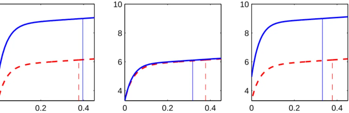
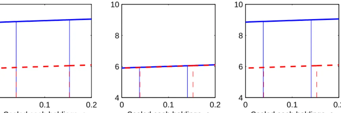
Figure 3 shows that similar results obtain in the refinancing case. Again the drift µ of permanent shocks affects mostly the value function and has little impact on optimal policies. The volatility σA of permanent shocks significantly affects optimal policies but has almost
Figure 3: The effects of permanent shocks with refinancing 0 0.1 0.2 4 6 8 10
Scaled cash holdings, c
Scaled firm value, F(c)
A. Effect of drift µ 0 0.1 0.2 4 6 8 10
Scaled cash holdings, c B. Effect of volatility σ A 0 0.1 0.2 4 6 8 10
Scaled cash holdings, c C. Joint effect of µ and σ A
Notes. Figure 3 plots firm value and target cash holdings in the refinancing case. The dashed curves represent the case with only temporary shocks (σA=µ= 0) in all panels. The solid curves
are with permanent shocks, with µ= 0.01 and σA = 0 in Panel A,µ= 0 and σA= 0.25 in Panel
B, and µ = 0.01 and σA = 0.25 in Panel C. The vertical lines depict the scaled issue size c and
target scaled cash holdings c∗. Input parameter values are as in Table 1.
3.2
Cash-flow sensitivity of cash
Corporate liquidity models featuring solely temporary shocks characterize optimal cash hold-ings and dividend policies using a constant target level of cash holdhold-ings (see e.g. Bolton, Chen, and Wang (2011), D´ecamps, Mariotti, Rochet, and Villeneuve (2011), or Hugonnier, Malamud, and Morellec (2015)). This generates the prediction that firms at the target dis-tribute all positive cash flows or, equivalently, that cash holdings are insensitive to cash flows. As firms off the target retain all earnings, the predicted propensity to save from cash flows is either one or zero. Our model generates a more realistic firm behavior at the target cash level and provides an explicit measure of the cash-flow sensitivity of cash.
To illustrate this feature, suppose that cash holdings are at the target level so that
Mt = c∗At. As we show below, this is a most relevant assumption since the bulk of the
probability mass of the stationary distribution of cash holdings is at the target level. Upon the realization of a cash flow shock dXt, profitability At changes in expectation by
E[dAt|dXt] =µAtdt+σAAt
ρ σXAt
Figure 4: Cash-flow sensitivity of cash 0.05 0.1 0.15 0.11 0.12 0.13 0.14 0.15
Short−term shocks volatility, σ X
Cash−flow sensivity of cash,
ε 0 0.2 0.4 0 0.05 0.1 0.15 0.2 0.25
Permanent shocks volatility, σ A 0 0.5 1 0 0.05 0.1 0.15 0.2 0.25 Persistence, ρ 0.1 0.2 0.3 0.12 0.14 0.16 0.18
Cash flow rate, α
Cash−flow sensivity of cash,
ε
0.01 0.02 0.03 0.14
0.15 0.16
Cash carry cost, λ
0 0.02 0.04 0.12 0.14 0.16 0.18 0.2
Fixed financing cost, φ
Notes. Figure 4 plots the effects of exogenous parameters on the cash-flow sensitivity of cash in the refinancing case. Input parameter values are given in Table 1.
Target cash holdings then change to c∗(At+dAt) and this change conditional on dXtcan be
expressed as E[c∗dAt|dXt] =c∗ µ− αρσA σX Atdt+ ρσAc∗ σX dXt. (38)
The sensitivity of target cash holdings to cash flow shocks is then captured by the coefficient
defined by
= ρσAc
∗
σX
. (39)
As the firm may not be able to stay at the target after a positive shock if this sensitivity exceeds 1 and may have excess cash after a negative shock if the sensitivity is less than 1, the sensitivity of actual cash holdings to positive shocks is+ = min{,1}and to negative shocks
is−= max{,1}. It should be stressed thatmeasures the sensitivity in expectation, as one
would obtain by regressing cash flows on cash holdings. An advantage of our bi-dimensional model is that, whenever the cash flow persistence is less than perfect (i.e. whenever ρ <
1), individual realizations of cash flows are not tightly linked to changes in cash holdings, consistent with observed behavior of firms.
The sensitivity of cash holdings to cash flow shocks is driven by the positive relation between profitability and the marginal value of cash (i.e. Vam =−acF00 ≥0), which implies
that the firm optimally retains a part of a positive cash flow shock if profitability increases. For this mechanism to work, a cash flow shock needs to be related to changes in profitability in expectation; this is true if cash flow persistence is non-zero. Without permanent shocks (i.e. when σA = 0) or without persistence of temporary shocks (i.e. when ρ = 0), the
cash-flow sensitivity of cash is zero. As shown by equation (39), the sensitivity in our model depends directly on the parameters of temporary and permanent shocks, ρ, σA, and
σX, and indirectly on the other parameters of the model via the target level of cash holdings
c∗. In particular, sincec∗ increases in the cost of refinancing, the cash-flow sensitivity of cash increases in external financing frictions, consistent with Almeida, Campello, and Weisbach (2004). Figure 4 presents the effects of various parameters of the model on our measure of the cash-flow sensitivity of cash in the refinancing case. The effect of cash carry cost λ on
indicates that the sensitivity decreases withinternal financing frictions. That is, the firm is less willing to save from cash flows if holding cash is expensive. Furthermore, the sensitivity increases in volatilities of both short-term and permanent shocks and in the persistence of cash flow shocks. The effect of σX on is due to the fact that an increase in the volatility
of short-term shocks increases target cash holdings c∗. Lastly, note that the values of in Figure 4 are in the range reported in Almeida, Campello, and Weisbach (2004).
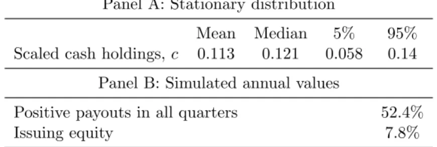
To support our claim that the bulk of the probability mass of the stationary distribution of cash holdings is at the target level, we next examine the stationary distribution of cash holdings implied by the model. This is done by simulating the model dynamics with the baseline parameter values in the refinancing case.10 Figure 5 and Table 2 present the results
Figure 5: Stationary distribution of scaled cash holdings 0 0.05 0.1 0 0.05 0.1 0.15 0.2 0.25
Scaled cash holdings, c
Notes. Figure 5 plots the stationary distribution of scaled cash holdings in the refinancing case. Input parameter values are given in Table 1.
and show that the stationary distribution of cash holdings is very skewed. The median level of cash reserves of 0.121 is close to the target level of cash reserves of 0.141. The concentration of cash holdings close to the target level arises for two reasons. One is the outcome of the optimal policies that attempt at warding off costly financial distress/refinancing. Second, and uniquely to our model, persistence in temporary shocks make safe firms even safer. This is related to the time varying volatility of scaled cash holdings. In our base case environment, this volatility decreases in c in the whole relevant domain. In particular, the volatility is the highest at low cash reserves and makes a firm in distress to quickly either recover with retained earnings or resolve to a new equity issuance. By contrast, a firm at the target cash level tends to stay there as the volatility of its scaled cash holdings is low. Panel B of Table 2 shows that the distribution of scaled cash reserves makes firms frequent and persistent dividend payers and infrequent equity issuers.
Table 2: Stationary distribution of scaled cash holdings.
Panel A: Stationary distribution
Mean Median 5% 95%
Scaled cash holdings, c 0.113 0.121 0.058 0.14 Panel B: Simulated annual values
Positive payouts in all quarters 52.4%
Issuing equity 7.8%
3.3
Investing in financially-constrained firms
A key result of Proposition 2 is that financing frictions reduce the value of an active firm and delay investment, in that the selected investment threshold for a constrained firm satisfies
a∗ > a∗F B. The results in Proposition 2 are therefore very different from those in prior studies, such as Boyle and Guthrie (2003), in which firms face financing constraints when seeking to invest in new projects. In such models, potential future financing constraints (i.e. potential future reductions in financial resources) feed back in current policy choices and encourage early investment. Our analysis therefore highlights another way by which financing constraints can distort investment behavior: The threat of future cash shortfalls increases future financing costs and reduces the value of the asset underlying the firm’s growth option, thereby leading to late exercise of the investment opportunity.
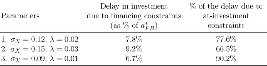
More generally, financing frictions have two separate effects on the timing of investment in our model. First, they increase the cost of investment, thereby delaying investment. Second, they reduce the value of an active firm (i.e. the value of the underlying asset), further delaying investment. Table 3 shows how these two effects vary with input parameter values. In our base case environment, Case 1 in the table, financing frictions increase the investment threshold by 7.8% and three quarters of the delay in investment is due to financing frictions at the time of investment and the remaining quarter due to expected future financing friction in the active firm. As shown by the table, a firm with more volatile cash flows (σX = 0.15)
and higher costs of holding cash (λ = 0.03) optimally invests at a yet higher threshold relative the first-best with one third of the delay coming from the post-investment financing
Table 3: Financing constraints and investment delay
Delay in investment % of the delay due to Parameters due to financing constraints at-investment
(as % of a∗F B) constraints
1. σX = 0.12, λ= 0.02 7.8% 77.6%
2. σX = 0.15, λ= 0.03 9.2% 66.5%
3. σX = 0.09, λ= 0.01 6.7% 90.2%
Notes. Table 3 presents the quantitative effects of financing constraints on the investment threshold and their decomposition. Input parameter values are given in Table 1.
frictions. A firm with a relatively low cash flow volatility and low costs of holding cash (Case 3) invests at a lower threshold but still much above the first-best threshold. In this case, the bulk of the delay is due to financing frictions at investment.
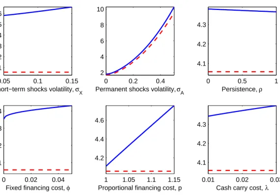
To provide a more complete picture, Figure 6 plots the selected investment thresholds for an unconstrained firm and for a constrained firm as functions of the volatilities of short-term and permanent shocks σX and σA, the persistence of cash flow shocks ρ, the proportional
cost of outside funds p, and the carry cost of cash λ. As shown by Figure 6, the effect of future financing constraints on investment policy increases with the carry cost of cashλ, the volatility of short-term shocksσX, and financing costs p, and decreases with the persistence
of cash flows ρ. Except for p, these effects are driven by the cost of financing frictions after investment and follow from the effects of these parameters on the value of an active firm.
A key difference between our model and traditional real options models is that firms face financing frictions and are exposed to short-term cash flow shocks. As discussed in Section 3.1.1, financing frictions and short-term shocks lead the firm to value inside equity and to hold cash balances at the time of investment as a precautionary motive. At the same time, however, financing frictions and the uncertainty associated with short-term shocks lead the firm to delay investment and, thus, to an increase in the value of productive assets at the time of investment. Figure 7 shows that the first effect is more important quantitatively in
Figure 6: Optimal investment threshold 0.05 0.1 0.15 4.1 4.2 4.3 4.4 4.5 4.6
Short−term shocks volatility, σ X Investment threshold, a * 0 0.2 0.4 2 4 6 8 10
Permanent shocks volatility, σ A 0 0.5 1 4.1 4.2 4.3 Persistence, ρ 0.01 0.02 0.03 4.1 4.2 4.3
Cash carry cost, λ 0 0.02 0.04
4.1 4.2 4.3 4.4
Fixed financing cost, φ
Investment threshold, a * 1 1.05 1.1 1.15 4.2 4.4 4.6
Proportional financing cost, p
Notes. Figure 6 plots the investment threshold a∗ in the refinancing case (solid curves) and in the first best (dashed curves). Input parameter values are given in Table 1.
our base case environment, so that comparative statics for the asset mix of the firm mirror those for target cash holdings at the time of investment.
Our model also has implications for the relation between investment and uncertainty. Notably, we have shown that an increase in the volatility of short-term shocks raises the risk of future funding shortfalls, thereby reducing the value of an active firm and investment incentives. Therefore, our model predicts that in most economic environments, increasingσX
will decrease investment rates. Another determinant of risk in our model is the persistence of cash flow shocks. Since an increase in the persistence of cash flows unambiguously increases the value of a constrained firm, another novel prediction of our model is that increasing ρ
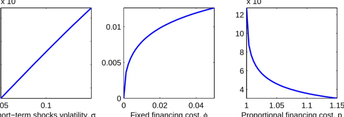
should increase investment rates. As shown by Figure 6, the effect is quantitatively small. Lastly, an interesting feature of our real options model is that the value function starts as
Figure 7: Optimal asset mix 0.05 0.1 2 3 4 5 x 10⁻³
Short−term shocks volatility, σ X Cash−to−Risky−assets 0 0.02 0.04 0 0.005 0.01
Fixed financing cost, φ
1 1.05 1.1 1.15 4 6 8 10 12 x 10−3
Proportional financing cost, p
Notes. Figure 7 plots the effects of financing frictions and volatility of temporary shocks on the asset mix of the firm at the time of investment. Input parameter values are given in Table 1.
G(a) before investment, a function of only a that is convex in a, and changes to V(a, m) =
aF(m/a) after investment, a function of a and m that is concave in a. One potential implication of this property is that the firm’s strategy with respect to asset risk (and exposure to shocks) would be different before and after investment. That is, before investment the firm, if it had a choice, would select assets/technologies with high risk. After investment, the firm would like to mitigate risk using the strategies described in Section 4 below.
3.4
Fixed issuance costs
We conclude this section with a discussion of the role of the scalability in a in our model. Many firm variables scale up as the firm grows and becomes more productive and profitable. We have used this observation to motivate our assumption that the fixed refinancing cost is proportional to the firm’s profitability a. As shown in Section 2.1, the ratio of cash holdings over profitability is the unique state variable for the firm’s problem in this case and the firm’s optimal policies can be fully characterized; see Proposition 1.
Suppose now that the fixed issuance cost is constant and does not depend on firm prof-itability a, so that the average equity issuance cost is lower for larger firms. Shareholders’ optimization problem then involves a difficult mixed control and stopping problem with two