Procedia Economics and Finance 5 ( 2013 ) 58 – 67
2212-5671 © 2013 The Authors. Published by Elsevier B.V.
Selection and/or peer-review under responsibility of the Organising Committee of ICOAE 2013 doi: 10.1016/S2212-5671(13)00010-5
International Conference On Applied Economics (ICOAE) 2013
Inflation, Economic Growth and Government Expenditure of
Pakistan: 1980-2010.
Muhammad Irfa
ff n
aa Javaid Attari
a*,
Attiya Y. Javed
d
baPh.D. Scholar, Shaheed Zulfikar Ali Bhutto Institute of Science and Technology (SZABIST), Islamabad, Pakistan.
a
bProfessor, Pakistan Institute of Development Economics (PIDE), Islamabad, Pakistan.
b
Abstract
This study is going to explore the relationship among the rate of inflation, economic growth and government expenditure in case of Pakistan. In this study, the government expenditure has been disaggregated in to the government current expenditure and the government development expenditure. This investigation is made by using the time series data during the period 1980-2010. The econometrics tools like Augmented Dickey Fuller (ADF) unit root test, ARDL, Johansen cointegration and Granger-causality test are used to investigate such relationship. The results derived by applying these econometrics tools show that there is a long term relationship between rate of inflation, economic growth and government expenditure, it means the government expenditures yield positive externalities and linkages. In the short run, the rate of inflation does not affect the economic growth but government expenditures do so. The causality test results show that there is unidirectional causality between rate of inflation and economic growth and; economic growth and government expenditure.
© 2013 Published by Elsevier Ltd. Selection and/or peer-review under responsibility of the Organising Committee of ICOAE 2013
Key words:Inflation; economic growth; government expenditure; ARDL;
1. Introduction
In the past few years in the economic history of Pakistan, the pace of economic growth is gradually decreasing but the size of government expenditure is gradually increasing. According the Handbook of Statistics on Pakistan Economy, 2010 published by State Bank of Pakistan (SBP), in 2009 the size of government expenditure increases to 9.41% from the previous year, but the GDP increases with 3.63% from © 2013 The Authors. Published by Elsevier B.V.
Selection and/or peer-review under responsibility of the Organising Committee of ICOAE 2013
ScienceDirect
Open access under CC BY-NC-ND license.
previous year. The condition is consider to be more worse, if we see the stat of 2008, the size of government expenditure increases to 40.76% from the previous year and GDP increases to 7.19%. The Table 1 shows the percentage change in the economic growth and government expenditure, the economic growth of Pakistan: Table 1 GDP and Government Expenditure: Pakistan 1980 to 2010
Year GDP Government Expenditure
In Million Rs. %age change In Million Rs. %age change
1980 1,265,370 7.327% 58,588 19.215% 1985 1,747,956 8.708% 119,832 15.408% 1990 2,295,202 4.589% 222,419 3.612% 1995 2,905,705 4.133% 421,736 15.767% 2000 3,562,020 4.868% 741,439 8.080% 2005 4,593,230 8.958% 1,001,006 11.407% 2009 5,767,536 3.632% 2,101,456 9.411%
In 2001 and 2003, the government was able to cut the government expenditure from the previous year by -4.502% and -9.288% respectively, the negative sign shows the reduction of expenditure from the previous year. In 2003 and 2004, the percentage change in GDP is greater than the government expenditure, i.e. the change in GDP is 4.726% and 7.483% respectively; and the change in the government expenditure is -9.288% and 4.335% respectively. As the government expenditure increases, there is need of more finances to meet such expenditures. Therefore, the government knocks at the door of international financial institutions like IMF, World Bank, Asian Development Bank; or borrows from the central bank like SBP; or imposes more taxes on the general public to meet their expenditure. In the previous literature, the ultimate effect of such loans or borrowings or imposing of such taxes had a serious negative impact on the economic growth of the country. According to Landau, 1985 the borrowing from the central bank, tend to increase the money supply, which is major reason of increasing the inflation and causes the uncertainty in the economy. The borrowing from the general public causes the interest rate to increase and reduces the further investment in the country. The enforcement of more taxes causes the distortion in the economy and reduces the output and growth.
The aim of this study is to complement the empirical investigation of inflation in Pakistan. More specifically:
x To measure the relationship between the rate of inflation and economic growth variable;
x To measure the relationship between the economic growth variable and aggregated government expenditure;
x To measure the relationship between economic growth variable, the rate of inflation and dis-aggregated government expenditure, i.e. government current expenditure and the government development expenditure; and
x To examine the direction of causal relationship among the inflation, economic growth and government expenditure.
The rest of paper is divided in the different sections: Section 2 reviews the literature. The methodology and model are explained in the Section 3. The Section 4 explains the analysis. In last, the Section 5 gives some conclusion and Section 6 gives some recommendations to the policy makers.
2.Literature Review
Gregorio, 1992: Fischer, 1993: Barro 1995; Thornton, 1996; Atesoglu, 1998; Bruno & Easterly, 1998; Ericsson, Irons & Tryon, 2001; Guerrero, 2006). According to them, if the rate of inflation exceeds the threshold level the growth nexus is strongly (negatively) affected by the inflation. Landu, 1983 and 1985 have measured the negative relationship between the government expenditure and economic growth and had suggested that the increase in the government expenditure is correlated with slowdown in economic growth among the developed countries.
Devarajan, Swaroop and Zou, 1996 had measured the negative relationship between the capital component of government expenditure and economic growth. They had disaggregated the government expenditure into the productive and unproductive expenditure. They had suggested that the expenditure which are considered to be productive but become unproductive, if they are in excessive amount. Loizidies and Vamvoukas, 2005 had measured the causal relationship between the size of public sector (i.e. ratio of government expenditure relative to GNP) and real per capita income. The results suggested that government expenditure causes real income both in long run and short run. In case of Greek, the increase in output causes growth in public expenditure.
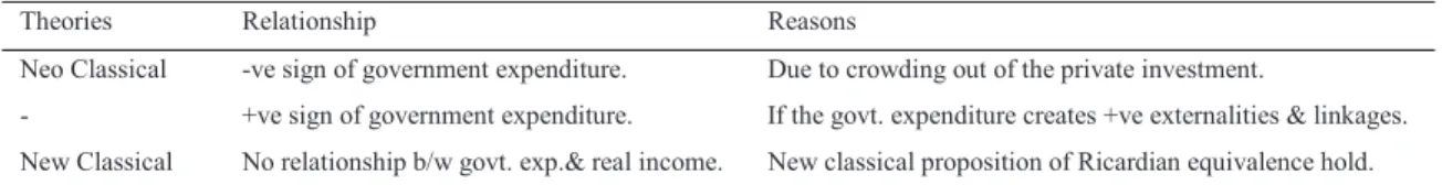
The relationship between economic growth and government expenditure might be positive or negative or no relation depending upon the effect of government expenditure as shown in Table 2.
Table 2 Relationship between Government Expenditure and Economic Growth
Theories Relationship Reasons
Neo Classical -ve sign of government expenditure. Due to crowding out of the private investment.
- +ve sign of government expenditure. If the govt. expenditure creates +ve externalities & linkages. New Classical No relationship b/w govt. exp.& real income. New classical proposition of Ricardian equivalence hold.
The negative relationship between the inflation rate and real income had been found, when the government expenditure was incorporated the expected sign between inflation and real income had changed. The positive relationship in long run had suggested that the moderate rise in the inflation should raise real income (Atesoglu, 1998; Mallik & Chowdhury, 2002). Atesoglu, 1998; and Mallik and Chowdhury, 2002 had used the government expenditure in the aggregated sense in their function form. But in this study, the government expenditure has been disaggregated into the government current expenditure and the government development expenditure as by Devarajan, Swaroop and Zou, 1996. The State Bank of Pakistan (SBP) has disaggregated the government expenditure into the Handbook of Statistics on Pakistan Economy, 2010.
3.Methodology and Model
This study builds on the work of Atesoglu, 1998; and Mallik and Chowdhury, 2002 by considering Pakistan perspective. This study also investigates the same relationship among the real GDP, rate of inflation and government expenditure, and follow the same function form as by Atesoglu, 1998; and Mallik and Chowdhury, 2002:
݈ܻ݊௧= ݂(ο݈݊ܲ௧, ݈݊ܩ௧) (3.1)
where:
lnY = the natural log of real GDP
ǻlnP = the rate of inflation, by taking the first difference of natural log CPI lnG = the natural log of real government expenditure
The equation (named as M-1) describes the relationship give below:
݈ܻ݊௧= ߚ+ߚଵο݈݊ܲ௧+ߚଶ݈݊ܩ௧+ߤ௧ (M-1)
study has also divided the government expenditures into: government current expenditures; and government development expenditures, according to the Handbook of Statistics on Pakistan Economy, 2010. First, the individual effect of both expenditures has been tested; and secondly, the combined effect of both expenditures has been taken by using the same equation (3.1). The three different equations (named as M-2, M-3 and M-4) are derived as follow:
݈ܻ݊௧= ߚ+ߚଵο݈݊ܲ௧+ߚଶ݈݊ܩܥ௧+ߤ௧ (M-2)
݈ܻ݊௧= ߚ+ߚଵο݈݊ܲ௧+ߚଶ݈݊ܩܦ௧+ߤ௧ (M-3)
݈ܻ݊௧= ߚ+ߚଵο݈݊ܲ௧+ߚଶ݈݊ܩܥ௧+ߚଷ݈݊ܩܦ௧+ߤ௧ (M-4) Where;
lnGC = the natural log of real government current expenditure lnGD = the natural log of real government development expenditure
Pesaran and Shin, 1999; and Perasan, Shin and Smith, 2001 had introduced a new method of testing for cointegration called the autoregressive distributed lag (ARDL) approach. This technique has been used in this study to measure the relationship among the economic variables, which include five different steps, are: x To verify the existence of unit root for each variable;
x To estimate the optimal lag orders criterion of every equation;
x To measure the long run relationship among the variables by using Wald test; x To estimate the coefficients both in long run and short run; and
x In the end, the diagnostic and stability test has been used.
The AIC lags criterion has been used in the ARDL model. The variable of real gross domestic product (Y), government expenditure (G), government current expenditure (GC) and government development expenditure (GD) are measured in local monetary unit (Rs.). The variable of rate of inflation (P) is measured in percentage change of log of consumer price index (CPI). The data for the all the economic variables has covered the period of 1980 to 2010 and has been taken from Handbook of Statistics on Pakistan Economy (2010).
4.Analysis
At the first step, ADF Unit Root test has been used to check that the economic variables are stationary. The ADF test includes constant with no trend at level I(0), and first difference I(1) of variables. The lag differences (k) are chosen according to Schwarz Info Criterion (SIC). The test results had shown in Table 3: Table 3 ADF Unit Root Test Statistic: Pakistan 1980 to 2010
Variable Level I(0) Level I(1)
No trend k No trend K ln(Y) -1.708 0 -3.497** 0 ln(P) -1.463 0 -5.123* 0 ln(G) -0.251 0 -6.540* 0 ln(GC) -0.654 0 -5.993* 0 ln(GD) 0.397 0 -4.670* 0
* and ** denotes MacKinnon critical values 1% and 5% significance at the level respectively.
The test result shown in Table 3, indicates that the time series data at level I(0) is nonstationary at 1% and 5% level of significance at different lags. The deterministic trend means that the time series is now completely predictable and not variable. So, all the times series of the variables are stationary in case of Pakistan, this implies that all the shocks that would be temporary and their effects would be eliminated over time as the
series regress to their long term variance. After finding all the economic variables that are integrated at order I(0) and order I(1), the second step of the ARDL cointegration test has been employed by the selection of the VAR optimal lag orders.
Table 4(a) Test Statistics and VAR Lag Order Selection Criterion of Model: (M-1 Endogenous Variables)
Order LL LR FPE AIC SC HQ
0 159.53 NA 4.11e-09 -10.79 -10.65* -10.75
1 170.99 19.97* 3.49e-09* -10.96* -10.39 -10.78*
2 176.33 8.09 4.60e-09 -10.71 -9.72 -10.40
Table 4(b) Test Statistics and VAR Lag Order Selection Criterion of Model: (M-2 Endogenous Variables)
Order LL LR FPE AIC SC HQ
0 156.62 NA 5.03-09 -10.59 -10.45* -10.55
1 168.12 19.84* 4.25e-09* -10.76* -10.20 -10.59*
2 175.08 10.55 5.01e-09 -10.62 -9.63 -10.31
Table 4(c) Test Statistics and VAR Lag Order Selection Criterion of Model: (M-3 Endogenous Variables)
Order LL LR FPE AIC SC HQ
0 147.77 NA 9.26e-09 -9.98 -9.84* -9.93
1 160.66 22.23* 7.12e-09* -10.25* -9.68 -10.07*
2 164.72 6.16 1.02e-08 -9.91 -8.92 -9.60
Table 4(d) Test Statistics and VAR Lag Order Selection Criterion of Model: (M-4 Endogenous Variables)
Order LL LR FPE AIC SC HQ
0 176.43 NA 8.04e-11 -11.89 -11.70* -11.83*
1 195.79 32.04* 6.47e-11* 12.12* -11.18 -11.82
2 204.85 12.50 1.12e-10 -11.64 -9.94 -11.11
*denotes lag order selected by the criterion; LL: log likelihood; LR:log likelihood ratio; FPE: Final prediction error; AIC: Akaike information criterion; SC: Schwarz information criterion; HQ: Hannan-Quinn information criterion
In order to select the optimal lag order for the VAR from the above Table 4 (a), (b), (c), (d), it is important to select high enough order to ensure that the optimal order will not exceed it. The three VAR of order two have been calculated over the time period of 1980 to 2010. However, AIC criteria implied that the order is 1. The log likelihood ratio statistics, whether adjusted for small sample or not, rejected order 0, but did reject a VAR of order 1. In the light of above statistics it has been decided to choose VAR (1) model.
After finalizing the selection of the VAR optimal lag orders, the third step of the ARDL cointegration test has been established of a long run relationship (cointegration) among the variables through F-test statistics by applying Bound Test. In the first stage, OLS is calculated to measure the long run relationship. At the second stage, F-statistics have been calculated by applying the Wald test on the estimation of OLS calculated at the first stage. The result of this step has been shown in Table 5:
Table 5 Wald Test: Pakistan 1980 to 2010
Model # F-statistics p-value
M-1 2.897* 0.096**
M-2 3.584* 0.022**
M-3 3.087* 0.050**
M-4 2.534* 0.078**
* the critical value ranges of F-statistics is 4.39-5.91, 3.17-4.45 and 2.63-3.77 at 1%, 5% and 10% level of significance respectively. ** denotes rejection of hypothesis at the 10% significance level.
Table 5 shows that F-statistic for order of lag one turned out to be significant at 10% level. The result implies the evidence that there is a strong long run relationship among the variables of the entire models.
After finding the long relationship among the variables, the fourth step is to estimate the long run and the short run coefficients. In the first stage, the long run coefficients have been estimated by using the OLS technique. The results of the long run estimates are shown in Table 6:
Table 6 ARDL Model Long Run Estimates: Pakistan 1980 to 2010 Model Long run estimates
M-1 lnY = 0. 058* - 0.210* οlnP + 0.072* lnG
M-2 lnY = 0. 060* - 0.201* οlnP + 0.051 lnGC
M-3 lnY = 0. 061* - 0.196* οlnP + 0.058* lnGD
M-4 lnY = 0.058* - 0.211* οlnP + 0.031 lnGC + 0.052* lnGD
*indicates 10% level of significance and figures in the brackets indicate standard errors.
The results that are presented in above Table 6 show that there is negative coefficient of rate of inflation, which is statistically significant. The same negative coefficient of inflation had also found in the case of UK. The coefficient of government expenditure is statistical positively significant and found same sign as it was in the case of Australia, Canada, Finland, New Zealand, Spain, Sweden, UK and US (Atesoglu, 1998; Mallik & Chowdhury, 2002). In model 2 and 4, the coefficient of government current expenditure is statistically insignificant. The coefficient of government development expenditure is statistically significant, in Model 3 and 4.
As the long-run estimates have been calculated, the short run (ECM) coefficients have been estimated in the next stage. The estimated results of ECM allow measuring the speed of the adjustments required to adjust to long run values after a short term shock. The short run results are shown in Table 7:
Table 7 ARDL Model ECM Estimates: Pakistan 1980 to 2010 Model Dependent Variable: οlnY
M-1 -0.001 - 0.042 οlnP + 0.065*οlnG - 0.775* ܧܥܯ(െ1)
M-2 -0.001 - 0.009 οlnP + 0.053*οlnGC - 0.765* ܧܥܯ(െ1)
M-3 -0.001 - 0.098 οlnP + 0.040*οlnGD - 0.868* ܧܥܯ(െ1)
M-4 -0. 001 - 0.070 οlnP + 0.040 οlnGC + 0.043 οlnGD - 0.883*ܧܥܯ(െ1)
The coefficient of error correction term (ECM) is -0.775, -0.765, -0.868 and -0.883; with the expected sign and significant p-value. However the ECM coefficient is fairly large and which implies that 77.5%, 76.5%, 86.8% and 88.3% of the disequilibria in the in GDP of the previous year’s shocks adjust back to the long run equilibrium in the current year.
The robustness of ARDL bound test of cointegration is checked by the Likelihood Ratio (LR) Tests in order to determine the number of cointegrating relationships proposed by Johansen, 1995. The test results of trace statistics tests, which is shown in Table 8.
Table 8 Cointegration Test Statistic for lnY: Pakistan 1980 to 2010
Model Eigen Value Hypothesized no. of CE ī
trace M-1 0.548 None * r=0 34.688* 0.261 $W0RVWU 11.636 0.094 $W0RVWU 2.874 M-2 0.578 None * r=0 37.208* 0.277 $W0RVWU 12.175 0.090 $W0RVWU 2.757 M-3 0.527 None * r=0 31.799* 0.223 $W0RVWU 10.049 0.089 $W0RVWU 2.729 M-4 0.600 None * r=0 59.580* 0.505 $W0RVWU 32.967* 0.294 $W0RVWU 12.571 0.080 $W0RVWU 2.438
* denotes rejection of hypothesis at the 5% significance level. MacKinnon-Haug-Michelis, 1999 p-values.
Table 8 reported that long run equilibrium exists between the variables (lnY, lnP, lnG, lnGC, & lnGD). Thus, it will be concluded that there is long relationship between the GDP, rate of inflation and government expenditure exist in terms of Pakistan. The trace statistics indicates that there are two numbers of cointegration equations at the 5% level which confirm the results of the Pesaran et al. (2001) cointegration approach.
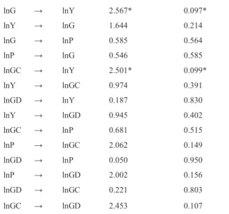
The Granger Causality test has been used to verify the direction of causality between the variables of Pakistan. It measures the two ways causality means the cause and effect relationship between two or more variables. The results are shown in Table 9:
Table 9 Granger Causality Results F-statistics: Pakistan 1980 to 2010
Variables F-statistics p-value
lnP ĺ lnY 3.092* 0.063*
lnG ĺ lnY 2.567* 0.097* lnY ĺ lnG 1.644 0.214 lnG ĺ lnP 0.585 0.564 lnP ĺ lnG 0.546 0.585 lnGC ĺ lnY 2.501* 0.099* lnY ĺ lnGC 0.974 0.391 lnGD ĺ lnY 0.187 0.830 lnY ĺ lnGD 0.945 0.402 lnGC ĺ lnP 0.681 0.515 lnP ĺ lnGC 2.062 0.149 lnGD ĺ lnP 0.050 0.950 lnP ĺ lnGD 2.002 0.156 lnGD ĺ lnGC 0.221 0.803 lnGC ĺ lnGD 2.453 0.107
*indicates the rejection of null hypothesis at 10% significant level.
The test results show that there is unidirectional causality between rate of inflation and GDP; government expenditure and GDP; and government capital expenditure and GDP. The test results also show that there is no directional causality between rate of inflation and government expenditure. In case of GDP and government current expenditure; and GDP and government development expenditure, there is also no causal relationship.
The model passed through the diagnostic tests like serial correlation and functional form specification. To investigate the serial correlation, the Breusch-Godfery Langrage Multiplier (LM) test is applied and the result has been concluded by allowing for up to one lag in Table 10:
Table 10 Breusch-Godfery Langrage Multiplier (LM) Test: Pakistan 1980 to 2010
Model # F-statistics p-value
M-1 0.686 0.512
M-2 0.737 0.488
M-3 0.184 0.832
M-4 0.148 0.862
* denotes rejection of hypothesis at the 10% significance level.
The results have suggested the acceptance of null hypothesis i.e. there is no serial correlation, it means that the disturbance term relating to any variable has not been influenced by the disturbance term relating to another variable.
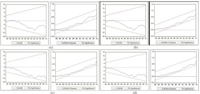
Finally, the model has passed through the stability test. The cumulative sum of recursive residuals (CUSUM) and the cumulative sum of squares of recursive residuals (CUSUMSQ) are used as the last stage of ARDL estimation to check that all coefficients in ECM model are stable or not. The plots of CUSUM and CUSUMSQ statistics are presented in Fig 1:
(a) (b)
(c) (d)
Fig. 1 Plot of CUSUM and CUSUMQ (a) M-1; (b) M-2; (c) M-3; (d) M-4
Fig 1 indicate the plot of cumulative sum of recursive residuals (CUSUM) and the cumulative sum of squares of recursive residuals (CUSUMSQ) that all the coefficients in the estimated ECM model are stable over the sample period at the 5% level of significant. And all the models can be evaluated for an effective policy analysis by the policy makers.
5.Conclusion
The relationship between inflation and economic growth has been the subject of extensive research over the past of few decades. This research is going to explore the same relationship among inflation, economic growth and government expenditure, in case of Pakistan. At the first step, unit root has been tested and the test results indicate that the time series data is stationary.
Secondly, ARDL has been used to measure the long run and short run estimates. The findings are disagreeing to the new classical proposition (Ricardian equivalence). The negative high coefficient of inflation had been found in the case of Pakistan, as in UK. It states that if the rate of inflation exceeds the threshold level the growth nexus is strongly (negatively) affected by the inflation. The estimated relationship between real income and government expenditure is positive and the same sign had been found in the case of Australia, Canada, Finland, New Zealand, Spain, Sweden, UK and US (Atesoglu, 1998; Mallik & Chowdhury, 2002).
As the government expenditure disaggregated into government current expenditure and government development expenditure, the coefficient of government current expenditure is statistically insignificant. But, the coefficient of government development expenditure is statistically significant, that shows that the government expenditures yield positive externalities and linkages.
The robustness has been tested by applying cointegration and the results reported that there is long run equilibrium exists between the variables. The Granger Causality test has been used to verify the direction of causality between the variables of Pakistan. The test results show that there is unidirectional causality inflation and economic growth. The test results also show that there is no causality between inflation and government expenditure. In case of economic growth and government expenditure there is unidirectional
causality.
The different diagnostics tests are used: to investigate the autocorrelation, the Breusch-Godfery Langrage Multiplier (LM) test is applied and the results have suggested that there is no autocorrelation. The model has passed through the stability test. The cumulative sum of recursive residuals (CUSUM) and the cumulative sum of squares of recursive residuals (CUSUMSQ) are used as the last stage of ARDL estimation to check that all coefficients in ECM model are stable and applicable for an effective policy analysis.
6.Recommendations
First, the negatively high coefficient of inflation has suggested the policy makers to reconsider about the existing macro-economic policy. The first priority of them are to control the inflation by introducing “Inflation First” policy because high and persistent inflation is consider as imposition of regressive tax on the poor people and adversely impact on the economic development. Secondly, In case of the developing countries, a lot of issue faced by the government, like: utilization and the miss-allocation of resources. If the government expenditures are utilized in the excess amount, the excessive capital (productive) expenditures become unproductive at the margin.
References
Asteriou, D., Hall, S. H., 2007. Applied Econometrics (1st ed).New York: PalgraveMacMillan. Atesoglu, H. S., 1998. Inflation and real income, Journal of Post Keynesian Economics 20, p. 487. Barro, R. J., 1995. Inflation and economic growth, Bank of England Quarterly Bulletin, p. 166.
Breusch, T., 1978. Testing for autocorrelation in dynamic linear models, Australian Economic Papers 17, p. 334. Bruno, M & Easterly, W., 1998. Inflation crises and long run growth, Journal of Monetary Economics 41, 3.
Devarajan, S., Swaroop, V., Zou, H., 1996. The composition of the public expenditure and economic growth, Journal of Monetary Economics 37, 313.
De Gregorio, J., 1992. The effects of inflation on economic growth: lessons from Latin America, European Economic Review 36, p. 417. Dickey, D. A., Fuller, W. A., 1979. Distribution of estimators for autoregressive time series with a unit root, Journal of American
Statistical Association 74, p. 427.
Enders, W., 2004. Applied Econometric Time Series (2nd ed). New York: John Wiley and Sons.
Ericsson, N. R., Irons, J. S., Tryon, R. W., 2001. Output and inflation in the long run, Journal of Applied Econometrics 16, p. 241. Fischer, S., 1993. The role of macro-economic facts in growth, Journal of Monetary Economics 32, p. 482.
Godfrey, L. G., 1968. Testing for higher order serial correlation in regression equation when the regressions contain lagged dependent variables, Econometrica 46, p. 1303.
Granger, C. W. J., 1969. Investigating causal relations by econometric models and cross spectral methods, Econometrica 7, p. 424. Guerrero, F., 2006. Does inflation cause poor long-term growth performance?, Japan and World Economy 18, p. 72.
Johansen, S., 1995. Likelihood-based interface in Conitegrated Vector Auto Regressive models. Oxford: Oxford University Press. Landau, D. L., 1983. Government expenditure and economic growth: a cross-country study, Southern Economic Journal 49, p. 783. Landau, D. L., 1985. Government expenditure and economic growth in the developed countries: 1952-76, Public Choice 47, 459. Loizidies, J., Vamvoukas, G., 2005. Government expenditure and economic growth: evidence from trivariate causality testing, Journal of
Applied Econometrics 8, p. 125.
Mallik, G., Chowdhury, A., 2002. Inflation, government expenditure and real income in the long run, Journal of Economic Studies 29, p. 240.
Pesaran, M. H., Shin, Y., 1999. An autoregressive distributed lag modeling approach to cointegration analysis. In: Storm, S. (Ed.), Econometrics and Economic Theory in 20th Century: The Ranger Frisch Centennial Symposium. Cambridge University Press, Cambridge Chapter 11.
Pesaran, M. H., Shin, Y., Smith, R. J., 2001. Bound testing approaches to the analysis of level relationships, Journal of Applied Econometrics 16, p. 289.
Phillips, P., Perron, P., 1988. Testing for a unit root in time series regression with I(1) processes, Biometrika 75, p. 335.
State Bank of Pakistan, 2010 Hand book of statistics of economy of Pakistan. Retrieved May 05, 2011, from SBP web site via access: http://www.sbp.org.pk
Thornton, D. L., 1996. The costs and benefits of price stability: an assessment of Howitt’s Rule, Federal Reserve Bank of St. Louis Review 78, p. 23.