O
PTIMAL
S
TABILIZATION
P
OLICY WITH
F
LEXIBLE
P
RICES
A
LEKSANDER
B
ERENTSEN
C
HRISTOPHER
W
ALLER
CES
IFO
W
ORKING
P
APER
N
O
.
1638
CATEGORY 6: MONETARY POLICY AND INTERNATIONAL FINANCE
DECEMBER 2005
An electronic version of the paper may be downloaded
• from the SSRN website: www.SSRN.com
CESifo Working Paper No. 1638
O
PTIMAL
S
TABILIZATION
P
OLICY WITH
F
LEXIBLE
P
RICES
Abstract
We construct a dynamic stochastic general equilibrium model to study optimal monetary stabilization policy. Prices are fully flexible and money is essential for trade. Our main result is that if the central bank pursues a long-run price path, thereby controlling inflation expectations, it can improve welfare by stabilizing short-run aggregate shocks. The optimal policy involves smoothing nominal interest rates which effectively smooths consumption across states. Failure to follow a long-run price path makes any stabilization attempt ineffective.
JEL Code: E4, E5.
Aleksander Berentsen University of Basel Department of Economics Petersgraben 51 4003 Basel Switzerland [email protected] Christopher Waller University of Notre Dame
Department of Economics and Econometrics 444 Flanner Hall
Notre Dame, IN 46556-5602 USA
December 14, 2005
We would like thank Ken Burdett, V.V. Chari, Allen Head, Cyril Monnet, Ed Nosal, Guillaume Rocheteau, Ted Temzelides, Harald Uhlig, Randall Wright for very helpful comments. The paper has also benefitted from comments by participants at several seminar and conference presentations. Much of the paper was written while Berentsen was visiting the University of Pennsylvania. We also thank the Federal Reserve Bank of Cleveland and the CES in Munich for research support.
1
Introduction
After a long period of inactivity, the last few years have seen a tremendous resurgence of research focusing on how to conduct optimal monetary policy. Nearly all of this work has come from the New Keynesian literature which, in the tradition of real business cycle models, constructs dynamic stochastic general equilibrium models to study optimal stabilization policy. What sepa-rates New Keynesian models from real business cycle models is their reliance on nominal rigidities, such as price or wage stickiness, that allows monetary policy to have real e¤ects. Without nominal rigidities there is no role for sta-bilization policy since money is neutral. From this research one is tempted to conclude that price stickiness is necessary to generate a role for stabilization policy. In this paper we show that this is not the case – there is a welfare improving role for stabilization policy even if prices are fully ‡exible.
We show that the critical element for e¤ective stabilization policy is the central bank’s control of long-run in‡ation expectations. By doing so monetary policy has real e¤ects even though prices are fully ‡exible. What is interesting about our result is that it is closely related to a key policy recommendation coming out of the New Keynesian models: “good” monetary policy requires a form of in‡ation targeting in order to control in‡ation expectations.1 In
the New Keynesian models controlling in‡ation expectations makes a central bank’s stabilization response to aggregate shocks more e¤ective. Our model makes a much stronger case for controlling expectations. When prices are fully ‡exible any stabilization policy is completely neutral without a price path target.
To show the importance of controlling in‡ation expectations, we construct a dynamic stochastic general equilibrium model where money is essential for
1See, for example, Woodford (2003) Chapters 1 and 7. Also see Clarida, Gali and Gertler
trade and prices are fully ‡exible.2 There are aggregate shocks to preferences
and technology. The existence of a credit sector generates a nominal interest rate that the monetary authority manipulates in its attempt to stabilize these shocks. Policy is optimal since the monetary authority maximizes the expected lifetime utility of the representative agent subject to the allocation being a competitive equilibrium.
The characteristics of the optimal stabilization policy are the following. It involves smoothing nominal interest rates and individual consumption across states. When the marginal cost of production is roughly constant, optimal policy is procyclical. An interesting implication of this policy is that the central bank is essentially providing an elastic supply of currency – when demand for liquidity is high, it provides additional currency and withdraws it when the demand for liquidity is low. Furthermore, stabilization works through a liquidity e¤ect. By injecting money the central bank lowers nominal interest rates, stimulating borrowing, which leads to higher consumption and production. On the other hand, if the central bank does not follow its targeted long-run price path, these injections simply raise in‡ation expectations and the nominal interest rate, as predicted by the Fisher equation. Finally, we show that zero nominal interest rates are an all-or-nothing policy. That is, unless a nominal interest rate of zero can be done for all states, it is optimal to never
set it to zero.
The paper proceeds as follows. In Section 2 we describe the environment. In Section 3 agents’optimization problems are presented and in Section 4 we derive the …rst-best allocation. In Section 5 we present the central bank’s maximization problem and derive the optimal monetary policy. Section 6 contains discussion of the results and Section 7 concludes.
2By essential we mean that the use of money expands the set of allocations (Kocherlakota
2
The Environment
The basic environment is that of Berentsen, Camera, and Waller (2004) which builds on Lagos and Wright (2005). We use the Lagos-Wright framework because it provides a microfoundation for money demand and it allows us to introduce heterogenous preferences for consumption and production while keeping the distribution of money balances analytically tractable. Time is discrete and in each period there are three perfectly competitive markets that open sequentially.3 Market 1 is a credit market while markets 2 and 3 are goods markets. There is a [0;1] continuum of in…nitely-lived agents and one perishable good produced and consumed by all agents.
At the beginning of the period agents receive a preference shock such that they either consume, produce or neither in the second market. With probabil-ityn an agent consumes, with probability s he produces and with probability 1 n s he does neither. We refer to consumers as buyers and producers as sellers.
In the second market buyers get utility "u(q) from q > 0 consumption, where " is a preference parameter and u0(q) >0, u00(q)< 0, u0(0) = +1 and
u0(1) = 0. Furthermore, we impose that the elasticity of utility e(q) = quu(0(qq)) is bounded. Producers incur utility cost c(q)= from producing q units of output where is a measure of productivity. We assume that c0(q) > 0, c00(q) 0 and c0(0) = 0.
Following Lagos and Wright (2005) we assume that in the third market all agents consume and produce, getting utility U(x) from x consumption, with U0(x)>0, U0(0) =1,U0(+1) = 0 and U00(x) 0.4 Agents can produce one
3Competitive pricing in the Lagos-Wright framework is a feature in Rocheteau and
Wright (2005) and Berentsen, Camera, and Waller (2005).
4As in Lagos and Wright (2005), these assumptions allow us to get a degenerate
distri-bution of money holdings at the beginning of a period. The di¤erent utility functionsU(:)
unit of the consumption good with one unit of labor which generates one unit of disutility. The discount factor across dates is 2(0;1).
To motivate a role for …at money, we assume that all goods trades are anonymous. In particular, trading histories of agents are private information, which rules out trade credit. Consequently, sellers require immediate compen-sation so buyers must pay with money. There is also no public communication of individual trading outcomes (public memory), which eliminates the use of social punishments to support gift-giving equilibria.
The …rst market is a credit market where agents can borrow or lend money at the nominal interest ratei. In contrast to the goods market, we assume the existence of a record-keeping technology so that …nancial trading histories are not private information. In all models with credit default is a serious issue. To focus on optimal stabilization, we simplify the analysis by assuming that some mechanism exists that ensures repayment of loans in the third market.5 One
can show that due to the quasi-linearity of preferences in market 3 there is no gain from multi-period contracts. Furthermore, since the aggregate states are revealed prior to contracting there is no private information about productivity or preferences. As a result, the one-period nominal debt contracts that we consider are optimal.
2.1
Aggregate shocks
To study the optimal response to aggregate shocks, we assume that n, s, and " are stochastic. The random variable n has support [n; n] 2 (0;1=2], s and consume in the last market.
5One possibility would be that agents require a particular ‘tool’to be able to consume
in market 2. This tool can then be used as collateral against loans in market 1 so that for su¢ ciently high discount factors repayment occurs with probability one.
In Berentsen et al. (2004) we derive the equilibrium when the only punishment for strategic default is exclusion from the …nancial system in all future periods.
has support [s; s] 2(0;1=2], has support [ ; ], 0 < < <1, and" has support ["; "], 0< " < " <1. Let ! = (n; s; ; ")2 be the aggregate state in market 1, where = [n; n] [s; s] [ ; ] ["; "] is a closed and compact subset on R4+. The shocks are serially uncorrelated. Let f(!) denote the density function of!.
Shocks to n and " are aggregate demand shocks, while shocks to s and are aggregate supply shocks. We call shocks to"and intensive margin shocks since they change the desired consumption of each buyer and the productivity of each seller, respectively, without a¤ecting the number of buyers or sellers. In contrast, shocks ton and s a¤ect the number of buyers and sellers.
2.2
Monetary Policy
Monetary policy has a long and short-run component. The long-run compo-nent focuses on the trend in‡ation rate. The short-run compocompo-nent is concerned with the stabilization response to aggregate shocks.
We assume a central bank exists that controls the supply of …at currency. We denote the gross growth rate of the money supply by =Mt=Mt 1 where Mt denotes the per capita money stock in market 3 in period t. The central bank implements its long-term in‡ation goal by providing deterministic lump-sum injections of money, Mt 1, at the beginning of the period. These transfers are given to the private agents. The net change in the aggregate money stock is given by Mt 1 = ( 1)Mt 1. If >1, agents receive lump-sum transfers of money. For <1, the central bank must be able to extract money via lump-sum taxes from the economy. For notational ease variables corresponding to the next period are indexed by+1, and variables corresponding to the previous period are indexed by 1.
The central bank implements its short-term stabilization policy through state contingent changes in the stock of money. Let 1(!)M 1 and 3(!)M 1
denote the state contingent cash injections in markets 1 and 3 received by private agents. Note that total injections at the beginning of the period are T = [ 1(!) + ]M 1. We assume that 1(!) + 3(!) = 0. In short, any injections in market 1 are undone in market 3. This e¤ectively means that the long-term in‡ation rate is still deterministic since M 1 is not state dependent. Consequently, changes in 1(!) a¤ect the money stock in market 2 without a¤ecting the long-term in‡ation rate in market 3.6 With
1(!)+ 3(!) = 0we are implicitly assuming the central bank chooses a path for the money stock in market 3. As we show later, this allows the central bank to control price expectations in market 3, which is critical for successful stabilization policy.
The state contingent injections of cash should be viewed as a type of re-purchase agreement – the central bank ‘sells’ money in market 1 under the agreement that it is being repurchased in market 3. Alternatively, 1(!)M 1 can be thought of as a zero interest discount loan to households that is repaid in the night market. If 1(!) < 0, agents would be required to lend to the central bank at zero interest. Since they can earn interest by lending in the credit market it is obvious that agents would never lend money to the central bank. Thus, 1(!)<0 is not feasible and so 1(!) 0 in all states. Finally, to ensure repayment of loans we assume the central bank has the same record-keeping and enforcement technologies as in the credit market. Thus, the only di¤erence between the central bank and the credit market is the ability of the central bank to print …at currency.
The precise sequence of action after the shocks are observed is as follows. First, the monetary injection M 1 occurs and the central bank o¤ers up to 1(!)M 1 units of cash per capita to agents at no cost. Then, agents move to the credit market where non-buyers lend their idle cash and buyers borrow
6Lucas (1990) employs a similar process for the money supply so that changes in nominal
money. Agents then move on to market 2 and trade goods. In the third market agents trade goods once again, all …nancial claims are settled and the central bank takes out 3(!)M 1 = 1(!)M 1 units of money.
3
First-best allocation
In a stationary equilibrium the expected lifetime utility of the representative agent at the beginning of period t is given by
(1 )W =U(x) x+
Z
fn"u[q(!)] (s= )c[(n=s)q(!)]gf(!)d!: The …rst-best allocation satis…es
U0(x ) = 1 and (1)
"u0[q (!)] = c0[(n=s)q (!)] for all !: (2)
These are the quantities chosen by a social planner who could force agents to produce and consume.
4
Monetary allocation
In period t, let P denote the nominal price of goods in market 3. It then follows that = 1=P is the real price of money. We study equilibria where end-of-period real money balances are time and state invariant
M = 1M 1 z; ! 2 : (3)
We refer to it as a stationary equilibrium. This implies that is not state dependent and so 1= =P=P 1 =M=M 1 = . This e¤ectively means that the central bank chooses a price path P = P 1 in market 3.
In what follows, we look at a representative period t and work backwards from the third to the …rst market to examine the agents’choices.
4.1
The third market
In the third market agents consume x, produce h, and adjust their money balances taking into account cash payments or receipts from the credit market. If an agent has borrowed l units of money, then he repays (1 +i)l units of money.
Consider a stationary equilibrium. Let V1(m; t) denote the expected life-time utility at the beginning of market 1with m money balances prior to the realization of the aggregate state !. Let V3(m; l; !; t) denote the expected lifetime utility from entering market 3 with m units of money and net bor-rowing l when the aggregate state is ! in period t. For notational simplicity we suppress the dependence of the value functions on the aggregate state and time.
The representative agent’s program is V3(m; l) = max
x;h;m+1
[U(x) h+ V1(m+1)] (4) s.t. x+ m+1 =h+ (m+ 3M 1) (1 +i)l;
where m+1 is the money taken into period t+ 1. Rewriting the budget con-straint in terms of hand substituting into (4) yields
V3(m; l) = [m+ 3M 1 (1 +i)l] + max
x;m+1
[U(x) x m+1+ V1(m+1)]: The …rst-order conditions areU0(x) = 1 and
1+ V
m
1 = 0; (5)
where the superscript denotes the partial derivative with respect to the argu-ment m. Note that the …rst-order condition for money has been lagged one period. Thus,Vm
1 is the marginal value of taking an additional unit of money into the …rst market in period t. Since the marginal disutility of working is
one, 1 is the utility cost of acquiring one unit of money in the third market of period t 1.
The envelope conditions are
V3m = ;V3l = (1 +i): (6) As in Lagos and Wright (2005) the value function is linear in wealth. The implication is that all agents enter the following period with the same amount of money.
4.2
The second market
At the beginning of the second market there are three trading types: buyers (b), sellers (s) and others (o). Accordingly, let V2j(m; l) denote the expected lifetime utility of an agent of trading typej =b; s; o. Letqbandqs, respectively, denote the quantities consumed by a buyer and produced by a seller and letp be the nominal price of goods.
A seller who holds m money and l loans at the opening of the second market has expected lifetime utility
V2s(m; l) = c(qs)= +V3(m+pqs; l);
where qs = arg maxqs[ c(qs)= +V3(m+pqs; l)]. Using (6), the …rst-order condition reduces to
c0(qs) = p ; ! 2 : (7) A buyer who hasmmoney andl loans at the opening of the second market has expected lifetime utility
V2b(m; l) ="u(qb) +V3(m pqb; l);
where qb = arg maxqb "u(qb) +V3(m pqb; l) s.t. pqb m. Using (6) and (7) the buyer’s …rst-order condition can be written as
where q = q(!)is the multiplier on the buyer’s budget constraint in state!. If the budget constraint is not binding, then "u0(q
b) = c0(qs), which means trades are e¢ cient. If it is binding, then "u0(q
b)> c0(qs)which means trades are ine¢ cient. In this case the buyer spends all of his money, i.e. pqb =m.
The marginal value of a loan at the beginning of the second market is the same for all agents and so
V2lj = (1 +i) ; (9) for j = b; s; o. Using the envelope theorem and equations (6) and (8), the marginal values of money forj =b and j =s; oin the second market are
V2mb = "u0(qb)=c0(qs) (10) V2ms = V2mo = : (11)
4.3
The …rst market
An agent who has m money at the opening of the …rst market has expected lifetime utility
V1(m) =
Z
[nV2b(mb; lb) +sV2s(ms; ls) + (1 n s)V2o(mo; lo)]f(!)d!; (12) where mj =m+T +lj, j =b; s; o. Once trading types are realized, an agent of typej =b; s; o solves
max
lj V2j(mj; lj) s.t. 0 mj:
The constraint means that money holdings cannot be negative. The …rst-order condition is
V2mj +V2lj + j = 0; !2 ;
where j = j(!)is the multiplier on the agent’s non-negativity constraint in state !. It is straightforward to show that buyers will become net borrowers
while the others become net lenders. Consequently, we have b = 0 and
s = o >0.
Using (9)-(11), the …rst-order conditions for j =b and for j = s; ocan be written as
"u0(qb) = c0(qs) (1 +i); !2 ; (13)
i = s = o; !2 : (14)
Note that if i= 0, trades are e¢ cient and if i >0, they are ine¢ cient.
Using the envelope theorem and equations (8), (13), and (14), the marginal value of money satis…es
V1m =
Z
[ "u0(qb)=c0(qs)]f(!)d!: (15)
Di¤erentiating (15) shows that the value function is concave in m.
4.4
Stationary Equilibrium
We now derive the symmetric stationary monetary equilibrium. In a sym-metric equilibrium all agents of a given type behave equally. Then, market clearing in market 2 implies
q(!) qb(!) = (s=n)qs(!); ! 2 ; (16) while in the credit market it implies that all buyers receive a loan of size
lb(!) =
(1 n) [1 + + 1(!)]M 1
n ; ! 2 : (17)
In any monetary equilibrium the buyer’s budget constraint must hold with equality in at least one state. In these states we have
(n= )q(!)c0[(n=s)q(!)] = (!)z: (18)
wherez = M is the real stock of money and (!) = [1 + + 1(!)]=(1 + ). It follows from (18) that in binding statesq(!; z)< q (!)whereq(!; z)is an
increasing function ofz. In non-binding states we haveq(!; z) =q (!)where q (!) solves (2).
Finally, use (5) to eliminate Vm
1 and (16) to eliminate qs from (15). Then, multiply the resulting expression by M 1 to get
=
Z "u0[q(!; z)]
c0[(n=s)q(!; z)] 1 f(!)d!: (19)
We can now de…ne the equilibrium as the value of z that solves (19). The reason is that once the equilibrium stock of money is determined all other endogenous variables can be derived.
De…nition 1 A symmetric monetary stationary equilibrium is a z that satis-…es (19).
5
Optimal stabilization
The central bank’s objective is to maximize the welfare of the representative agent. It does so by choosing the quantities consumed and produced in each state subject to the constraint that the chosen quantities satisfy the conditions of a competitive equilibrium. The policy is implemented by choosing state contingent injections 1(!)and 3(!) accordingly.
The Ramsey problem facing the central bank is M x
q(!);x U(x) x+
Z
fn"u[q(!)] (s= )c[(n=s)q(!)]gf(!)d! (20) s.t. (19);
where the constraint facing the central bank is that the quantities chosen must be compatible with a competitive equilibrium. It is obvious thatx=x so all that remains is to chooseq(!).
Proposition 1 If = , the optimal policy is i(!) = 0 with q(!) = q (!) for all states.
According to Proposition 1, if = is feasible, the central bank should implement the Friedman rule i(!) = 0 for all states. The reason is that the only friction in our model is the cost of holding money across periods and the Friedman rule eliminates it. So agents can perfectly self-insure against all consumption risk. Consequently, there are no welfare gains from stabilization policies.7
Now consider the case in which > . For this case we have the following result.
Proposition 2 If > , the optimal policy is i(!) > 0 with q(!) < q (!) for all states.
Surprisingly, in this case the central bank never chooses i(!) = 0 for any state. The reason is that the central bank wants to smooth consumption across states. Intuitively, consider two states!; !0 2 withi(!) = 0implying
q(!) = q (!) and i(!0) > 0 implying q(!0) < q (!0). Then, the …rst-order loss from decreasingq(!)is zero while there is a …rst-order gain from increasing q(!0). This gain can be accomplished by increasing i(!) and lowering i(!0). Thus, the central bank’s optimal policy is to smooth interest rates across states.
According to Propositions 1 and 2, unless i(!) = 0 can be done for all
states, it is optimal to never set i(!) = 0. Hence, zero nominal interest rates should be an all-or-nothing policy. An interesting implication of the optimal policy is that the central bank is essentially providing an elastic supply of currency –when demand for liquidity is high, it provides additional currency and withdraws it when the demand for liquidity is low.8
7Ireland (1996) derives a similar result in a model with nominal price stickiness. He
…nds that at the Friedman rule there is no gain from stabilizing aggregate demand shocks.
8In an earlier version of the paper we analyzed the case where the aggregate shocks were
This striking di¤erence in the optimal policies raises the question of why a central bank might deviate from the Friedman rule. Deviations may oc-cur because the central bank is prevented from running the Friedman rule or chooses not to run it. The inability to run the Friedman rule may occur in environments with limited enforcement. In such environments all trades must be voluntary and so lump-sum taxes of money are impossible because the cen-tral bank cannot impose any penalties on the agents (see Kocherlakota 2001).9
On the other hand, the central bank might not choose to run the Friedman rule because it is not the optimal policy. For example, the Friedman rule can be suboptimal in models that display matching externalities (see Berentsen, Rocheteau and Shi (2004), Rocheteau and Wright (2005)). Another reason the central bank might be constrained from implementing the Friedman rule is that there are seigniorage needs implying >1. Since our focus is stabiliza-tion policy we have not explicitly modeled reasons that give rise to deviastabiliza-tions from the Friedman rule. Nevertheless, we conjecture the logic of Proposition 2 still applies in any model where the Friedman is not implemented.
5.1
An example
To illustrate how the optimal policy is implemented, consider a simple example in which the only shock is the intensive margin demand shock ". Let " be uniformly distributed and let preferences be given by u(q) = 1 exp q and c(q) = q. With these functions the …rst-order conditions for the planner (26)
9There is a di¤erence between lump-sum taxation and loan repayment. Voluntary loan
repayment can be supported with reputational strategies (see for example Berentsen, Cam-era, and Waller 2004). The reason is that default results in exclusion from …nancial markets and the loss of future bene…ts. In contrast, taxes typically …nance public goods for which exclusion is not possible thus taxes must necessarily be forced on individual agents by society.
(see Appendix) yields10
"exp q = n
n ; (21)
where is multiplier on the planner’s constraint. Substituting this expression in the central bank’s constraint we have
=
Z " "n
f(")d"=
n :
Solving for and substituting back into (21) yields
q(") = ln " ln ( = ) = q (") ln ( = ); (22) where q(") is increasing in ".11 Furthermore,
i(!) = :
Note that this implies perfect interest rate smoothing by the central bank. This is a special outcome due to the functional form of the utility and cost functions since in general the interest rate is not constant.
From the buyer’s budget constraint we have q(") = [1 + + 1(")]z
n(1 + ) : (23)
Sincez is not state dependent, taking the ratios of (23) for allq(")relative to q(") gives
q(") = 1 + + 1(") 1 + + 1(")
q("): (24) There is one degree of freedom in 1(") so let 1(") = 0. Thus
z = (n= ) [ln " ln ( = )] and using (22) and (24) gives
1 + 1(") 1 + =
ln " ln ( = )
ln " ln ( = ) >1 for all " > "; so 1(")>0for all " > ".
10With these utility and cost functions, the second-order condition is satis…ed.
11Since the Inada condition does not hold for this utility functionq(") = 0when = ":
6
Discussion
In this section we discuss why stabilization policy requires control of price expectations and we explore the gains from optimal stabilization by comparing the allocations under the optimal policy with the one when the central bank is passive. Finally we discuss a benchmark with “sticky” prices.
6.1
Liquidity and in‡ation expectation e¤ects
The optimal stabilization policy in our model works through a liquidity e¤ect. For this e¤ect to operate, the central bank must control in‡ation expectations by choosing a price path in market 3. Without it, injections in the …rst market simply change price expectations and the nominal interest rate as predicted by the Fisher equation.
To see this note from (13) that the interest rate associated with the optimal policy is
i(!) = "u
0[q(!)]
c0[(n=s)q(!)] 1>0, ! 2 : (25)
Assume for simplicity that the marginal cost is constant and equal to 1. Then rewrite the buyers budget constraint (18) and (25) to get
q(!) = ( =n) [1 + + 1(!)] M 1 and i(!) = "u0[q(!)] 1>0; !2 :
Since the central bank has committed to a price path for , changes in 1(!) do not a¤ect in the …rst equation. Hence, M 1 is constant. It then follows that increasing 1(!) raises real balances for all agents. This decreases the real demand for loans and increases the real supply of loans. As a result, the nominal interest rate falls lowering the cost of borrowing and soq(!)increases. Consequently, state contingent injections are not neutral as long as changes in
What happens if the central bank never undoes the state contingent injec-tions of market 1? In this case 3(!) = 0 for all t and ! 2 . We can then state the following
Proposition 3 Assume that 3(!) = 0 for all ! 2 . Then, changes in 1(!) have no real e¤ects and any stabilization policy is ine¤ective.
If the central bank does not reverse the state contingent injections of the …rst market, the price of goods in market 1 changes proportionately with changes in 1(!). Consequently, the real money holdings of the buyers are una¤ected and so consumption in market 1 does not react to changes in 1(!). Such a policy only a¤ects the expected nominal interest rate. To see this note that the gross growth rate of the money supply is t = 1(!) + + 1. Then substitute this and (25) into the constraint of the central bank problem to get
1(!) + + 1
=
Z
i(!)dF (!):
An increase in 1(!) increases the expected nominal interest rate. This is simply the in‡ation expectation e¤ect from the Fisher equation.
6.2
The ine¢ ciency of a passive policy
What are the ine¢ ciencies arising from a passive policy? In order to study this question we now derive the allocation when the central bank follows a policy where the injections are not state dependent, i.e., 1(!) = 3(!) = 0, and compare it to the central bank’s optimal allocation. We do so under the assumption that the central bank cannot use lump-sum taxes meaning 1. We also analyze each shock separately to understand their individual e¤ects on the equilibrium allocation.
Extensive margin demand shocks For the analysis of shocks to n, we assume that , " and s are constant. Note that the …rst-best quantity q (n) is non-increasing inn.
Proposition 4 For 1, a unique monetary equilibrium exists with q = q (n)ifn n~ andq < q (n)ifn > ~n, where~n2(0; n]. Moreover,dn=d <~ 0: With a passive policy buyers are constrained when there are many bor-rowers (highn) and are unconstrained when there are many creditors (lown). Since dn=d~ < 0, the higher is the in‡ation rate, the larger is the range of shocks where the quantity traded is ine¢ ciently low. Note that for large we can have n~ n which implies that q < q (n) in all states.
How does this allocation di¤er from the one obtained by following an active policy? We illustrate the di¤erences in Figure 1 for a linear cost function. The curve labelled “Passiveq”represents equilibrium consumption under a passive policy and the curve labelled “Active q” consumption when the central bank behaves optimally.
As shown earlier, with an active policy buyers never consumeq , and with linear cost equilibrium consumption q is increasing in n. This is just the opposite from what happens when the central bank is passive. With a passive policy, buyers consume q = q in low n states and q < q in high n states. Moreover, q is strictly decreasing in n for n > n~. These di¤erences are also re‡ected in the nominal interest rates. With an active policy the nominal interest rate is strictly positive in all states and decreasing in n. In contrast, with a passive policy the nominal interest rate is i = 0 for n n~ and i = " u0(q) 1 0 for n >n~, and increasing in n.
n _ n ñ q* q n shocks Passive q Activeq i = 0 i > 0
Figure 1: Shocks to the number of buyers.
What is the role of the credit market? With a linear cost function and no credit market, the quantities consumed are the same across all n-states since buyers can only spend the cash they bring into market 1, which is independent of the state that is realized. In contrast, with a credit market, idle cash is lent out to buyers. This makes individual consumption higher on average but also more volatile. The reason is that when n is high demand for loans is high and the supply of loans is low. This pushes up the nominal interest rate and decreases individual consumption. The opposite occurs when n is low.
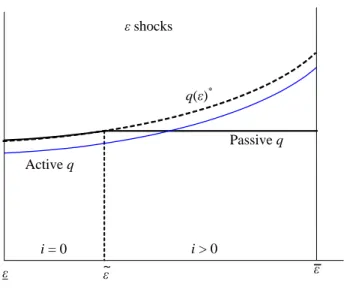
Intensive margin demand shocks To study " shocks we assume that , n and s are constant. It then follows that ! = ". Note that the …rst-best quantityq (")is strictly increasing in ".
Proposition 5 For 1, a unique monetary equilibrium exists with q < q (")for" >~"andq =q (")for" <~", where~"2[0; "]. Moreover,d~"=d <0.
With a passive policy, buyers are constrained in high marginal utility states but not in low states. If is su¢ ciently high, buyers are constrained in all
states. Note that with a passive policy dq=d" > 0 for " ~" and dq=d" = 0 for " > ~". For " ~", buyers have more than enough real balances to buy the e¢ cient quantity. So when " increases, they simply spend more of their money balances. For " > ~", buyers are constrained. So when " increases, the demand for loans increases but the supply of loans is unchanged so no additional loans can be made. Thus, the interest rate simply increases to clear the credit market.
~ q( )* _ shocks q Activeq i > 0 i = 0 Passiveq
Figure 2: Marginal utility shocks.
Figure 2 illustrates how the allocation resulting from a passive policy di¤ers from the one obtained under an active policy. The dashed curve represents the …rst-best quantitiesq ("). The curve labelled “Passiveq”represents equi-librium consumption under a passive policy and the curve labelled “Active q” consumption when the central bank behaves optimally. The central bank’s optimal choice is strictly increasing in ".
Finally, we have also derived the equilibrium under a passive policy for the extensive, s, and the intensive, , supply shocks. The results and …gures are qualitatively the same and we therefore do not present them here. They
typically involve a cuto¤ value such that the nominal interest rate is zero either above or below this value. These derivations are available by request.
6.3
A benchmark with "sticky" prices
With = 1 and a linear cost function prices of goods are constant across periods and within a period for shocks to n, ", and s. This benchmark is interesting because it mimics a sticky price model. However, the models look similar from the outset only since in our model prices always adjust to clear markets.
How does the optimal policy look like for this benchmark? First of all, Proposition 2 continues to hold, so q(!) < q (!). We …nd that the opti-mal policy is procyclical, in the sense that in response to aggregate demand shocks that drive interest rates up, the central bank intervenes to bring them back down. It is straightforward to construct examples where aggregate con-sumption and interest rates are negatively correlated. This is counter to the standard view that typically comes out of Keynesian models that the central bank should increase interest rates in response to positive shocks to aggre-gate demand. With convex cost, these results could be reversed due to price movements in market 2. Nevertheless, we have constructed examples with substantial convexity in the cost function, yet aggregate output and interest rates were negatively correlated.
Finally, our model has some interesting implication for in‡ation targeting. With convex costs in market 2, prices in market 2 will typically ‡uctuate in response to aggregate shocks. But it is optimal for the central bank to ignore these price ‡uctuations since it only aims to control in‡ation in market 3. Thus our model suggests that the central bank need only to target a subset of prices in the economy for optimal stabilization purposes. In some sense this is equivalent of targeting a core in‡ation rate.
7
Conclusion
In this paper we have constructed a dynamic stochastic general equilibrium model where money is essential for trade and prices are fully ‡exible. Our main result is that if the central bank targets a long-run price path, it can success-fully stabilize short-run aggregate shocks to the economy and improve welfare. The optimal policy works through a liquidity e¤ect and involves smoothing nominal interest rates, thereby smoothing consumption across states. If it does not adhere to the price path, stabilization attempts are ine¤ective. Mon-etary injections simply raise price expectations and the nominal interest rate as predicted by the Fisher equation.
There are many extensions of this model that would be interesting to pur-sue. For example, how would the optimal policy be a¤ected if repayment of loans were endogenous? In particular, does the risk of default alter stabiliza-tion? Furthermore, we have assumed that the shocks are known to the central bank. An interesting question is what is the optimal policy if the central bank has imperfect information about the nature of the aggregate shocks? A fur-ther extension would be to incorporate capital into the model to generate an intertemporal trade-o¤ for the optimal policy. Finally, how would the exis-tence of inside money a¤ect the equilibrium and optimal policy. For example, would inside money act as an automatic stabilizer, eliminating the need for the central bank to stabilize the economy? We leave this to future research.
Appendix
Proof of Proposition 1. From (20) the unconstrained optimum corre-sponds to q = q (!) for all ! = . From the constraint of the central bank problem, since < is not feasible, the only value that is consistent with the unconstrained optimum is = .
Proof of Proposition 2. The …rst-order conditions for the central bank are n"u0[q(!)] (n= )c0[(n=s)q(!)] + (!) = 0 ! 2 , (26)
where
(!) = " u
00[q(!)]c0[(n=s)q(!)] (n=s)c00[(n=s)q(!)]u0[q(!)]
c0[(n=s)q(!)]2 <0:
Note that is independent of !. Su¢ cient conditions for a maximum are "u00[q(!)] (n=s)c00[(n=s)q(!)] f "u0[q(!)] c0[(n=s)q(!)]g (!)<0; where (!) = u 000[q(!)]c0[(n=s)q(!)] (n=s)2 c000[(n=s)q(!)]u0[q(!)] u00[q(!)]c0[(n=s)q(!)] (n=s)c00[(n=s)q(!)]u0[q(!)] 2 (n=s)c00[(n=s)q(!)] c0[(n=s)q(!)]
for all ! 2 . The rest of the proof immediately follows from inspecting the …rst-order conditions (26).
Proof of Proposition 3. In any equilibrium buyers’money holdings are M 1[1 + + 1(!)] +lb(!) =
M 1[1 + + 1(!)]
n =
M(!) n ;
since the end-of-period nominal money stock isM(!) = M 1[1 + + 1(!)]. Thus, in any equilibrium we must have
(!)p(!)q(!) (!)M(!)
The …rst-order conditions of the sellers (7) imply 1c0[(n=s)q(!)]q(!) (!)M(!)
n ; !2 .
In a steady-state equilibrium (!)M(!) = 1(!)M 1(!) = z(!) for all ! 2 . Hence,
1c0[(n=s)q(!)]q(!) z(!)
n ; !2 . (27)
We now show that in any stationary equilibrium z(!) =z is a constant. Use (5) to eliminate Vm
1 and (16) to eliminate qs from (15) to get
1(! 1)= =
Z
f (!) "u0[q(!)]=c0[(n=s)q(!)]gf(!)d!:
Multiply this expression byM 1(! 1)to get M 1(! 1) 1(! 1)= =
Z M(!) (!)
(!)
"u0[q(!)]
c0[(n=s)q(!)] f(!)d!:
since M(!) = [1 + + 1(!)]M 1(! 1) = (!)M 1(! 1). Note that in any steady-state equilibrium the right-hand side is independent of ! 1 and therefore a constant. This immediately implies that M 1(! 1) 1(! 1) = z 1 is constant for all ! 1 2 . Since in a stationary equilibrium we have z 1 =z we can rewrite this equation as follows
1= =
Z "u0[q(!)]
(!)c0[(n=s)q(!)] f(!)d!:
Finally from (27) we have
1c0[(n=s)q(!)]q(!) z
n; !2 .
Since the right-hand side is independent of (!), changes is (!) are neutral. Hence, stabilization policy is ine¤ective.
Lemma 1 Under e¢ cient trading, real aggregate spending n p(!)q (!) is increasing in ". It is increasing in n and decreasing in s and if
= 1 + q u
00(q )
u0(q )
q c00[(n=s)q ] (n=s) c0[(n=s)q ] <0:
Proof of Lemma 1. In equilibrium buyer’s real money holdings are ( =n)z = z=n since = 1 with a passive policy. Thus, in any equilibrium n pq z. The right-hand side is the aggregate real money stock in market 1 which is independent of !. The left-hand side is real aggregate spending measured in market 3 prices which is a function of !. For a given state !, trades are e¢ cient if n p(!)q (!) z and ine¢ cient if n p(!)q (!) > z where p = p(!) is a function of ! but is not. We would like to know how real aggregate spending g(!) = n p(!)q (!) changes in ! when trades are e¢ cient:
dg(!) = p(!)q (!)dn+n q (!)dp+n p(!)dq :
The …rst term re‡ects the change in real liquidity that is intermediated in the economy. This e¤ect only occurs if n changes. The second term re‡ects changes in the relative price p of goods and the third term changes in the e¢ cient quantity. Rewrite it as follows
dg(!) =n pq dn n + dp p + dq q : The term dpp can be derived from (7) as follows
dp p = c00[(n=s)q ] c0[(n=s)q ] q n s dn n ds s d
and the term dqq can be derived from " u0(q ) =c0[(n=s)q ]as follows
dq q = c00[(n=s)q ] (n=s) "u00(q ) c00[(n=s)q ] (n=s) dn n ds s " u0(q )=q "u00(q ) c00[(n=s)q ] (n=s) d +d" " :
Investigating each shock separately we get @g(n) @n = c 0[(n=s)q ]q (n= s) 1 + c00[(n=s)q ] "u00(q ) c00[(n=s)q ] (n=s) 0 @g(n) @s = c0[(n=s)q ]q (n=s)2c00[(n=s)q ] f "u00(q ) c00[(n=s)q ] (n=s)g 0 @g(n) @ = c0[(n=s)q ]n"u0(q ) f "u00(q ) c00[(n=s)q ] (n=s)g <0 @g(n) @" = c0[(n=s)q ]nu0(q ) "u00(q ) c00[(n=s)q ] (n=s) >0:
Proof of Proposition 4. Here! =n.
Critical value: From (19) we have =
Z n n
"u0[q(n; z)]
c0[(n=s)q(n; z)] 1 f(n)dn: (28)
Lemma 1 gives @g@n(n) 0. If g(n) > z, then agents are constrained in all states. If g(n) < z, then agents are never constrained. If g(n) z g(n), for a given value of z there is a unique critical value ~n such that
g(~n) =z: (29)
This implies that q = q (n) for n n~ and q < q (n) for n > ~n. Note that @n~
@z 0.
Existence: Using (29) we can write (28) as follows =
Z n n
"u0[q(n; z)]
c0[(n=s)q(n; z)] 1 f(n)dn RHS; (30)
where n= maxfn; n~ g. Only the right-hand side is a function ofz. Note that lim
z!0RHS = 1. For z = g(n) we have n~ = n and therefore RHSjz=z = 0 . Since RHS is continuous in z an equilibrium exists.
Uniqueness: The right-hand side of (30) is monotonically decreasing in z. To see this use Leibnitz’s rule to get
@RHS @z = Z n n "[u00c0 (n=s)c00u0] (c0)2 @q(n; z) @z f(n)dn "u0[q(n; z)] c0[(n=s)q(n; z)] 1 f(n) @n @z:
Since q(n; z) = q (n)by construction we have @RHS @z = Z n n "[u00c0 (n=s)c00u0] (c0)2 @q(n; z) @z f(n)dn < 0:
Since the right-hand side is decreasing in z, we have a unique z that solves (30). Consequently, we have
q =q (n) if n n and q < q (n) otherwise.
Hours worked: Finally, if buyers have been constrained in market 1 money holdings at the opening of the third market arem3 =pqsfor sellersm3 = 0for non-sellers. Solving for equilibrium consumption and production in the third market, withx =U0 1(1), gives
hb = x +nec(q)c[(n=s)q] + (1 n)eu(q)u(q) hs = x nec(q)c[(n=s)q] (1 s)s 1 neu(q)u(q) ho = x +nec(q)c[(n=s)q] neu(q)u(q):
Notice that nhb+shs+ (1 n s)ho=x . Moreover, we havehb ho hs. For existence we need that all agents work a positive amount in the third market. This, it is su¢ cient to show that hs >0.
Given s > 0, n=s is bounded and since the elasticities ec(q) and eu(q) are bounded, we can scale U(x) such that there is a value x = U0 1(1) greater than the last term for all q 2 [0; q ]. Hence, hs is positive for for all q2[0; q ]ensuring that the equilibrium exists. Note that the states where the buyers are constrained are the ones where the sellers have all the money after trading. Therefore, if hs is positive in constrained states it is positive in all unconstrained states.
Proof of Proposition 5. Here! =".
Critical value: From (19) we have =
Z " "
"u0[q("; z)]
Lemma 1 gives @g@"(") 0. Ifg(")> z, then agents are constrained in all states. Ifg(")< z, then agents are never constrained. If g(") z g("), for a given value ofz there is a unique critical value ~" such that
g(~") = z: (32) This implies that q = q (") for " "~ and q < q (") for " > ~". Note that
@~"
@z 0.
Existence: Using (32) we can write (31) as follows =
Z " "
"u0[q("; z)]
c0[(n=s)q("; z)] 1 f(")d" RHS; (33)
where " = maxf~"; "g. Only the right-hand side is a function of z. Note that lim
z!0RHS = 1. For z = g(") we have ~" = " and therefore RHSjz=z = 0 . Since RHS is continuous in z an equilibrium exists.
Uniqueness: The right-hand side of (33) is monotonically decreasing in z. To see this use Leibnitz’s rule and note that by constructionq("; z) = q (") to get @RHS @z = Z " " "[u00c0 (n=s)c00u0] (c0)2 @q("; z) @z f(")d" <0:
Since the right-hand side is strictly decreasing in z, we have a uniquez that solves (33). Consequently, we have
q=q (") if " " and q < q (") otherwise.
Finally, it is straightforward to show that the hours worked in market 3 are bounded away from zero.
References
Berentsen, A., G. Camera and C. Waller (2004), “Money, Credit and Banking,” IEW Working Paper No. 219.
Berentsen, A., G. Camera and C. Waller (2005). “The Distribution of Money Balances and the Non-Neutrality of Money,”International Economic Review, 46, 465-487.
Berentsen, A., G. Rocheteau and S. Shi (2004), “Friedman Meets Hosios: E¢ ciency in Search Models of Money,”Economic Journal, forthcoming. Clarida, R., J. Gali and M. Gertler (1999). “The Science of Monetary Policy: A New Keynesian Perspective,”Journal of Economic Literature XXXVII, 1661-1707.
Ireland, P. (1996). “The Role of Countercyclical Monetary Policy,”Journal of
Political Economy 104 vol. 4, 704-723.
Lagos, R. and R. Wright (2005). “A Uni…ed Framework for Monetary Theory and Policy Evaluation,”Journal of Political Economy 113, 463-484.
Lucas, R. (1990). “Liquidity and Interest Rates,”Journal of Economic Theory
50, 237-264.
Kocherlakota, N. (1998). “Money is Memory,”Journal of Economic Theory,
81, 232–251.
Kocherlakota, N. (2001). “Money: What’s the Question and Why We Care About the Answer,” Sta¤ paper,Federal Reserve Bank of Minneapolis. Rocheteau, G. and R. Wright (2005). “Money in Search Equilibrium, in Com-petitive Equilibrium and in ComCom-petitive Search Equilibrium,”Econometrica, 73, 175-202.
Wallace, N. (2001). “Whither Monetary Economics?”International Economic Review, 42, 847-869.
Woodford, M. (2003). “Interest and Prices: Foundations of a Theory of Mon-etary Policy,” Princeton University Press.
CESifo Working Paper Series
(for full list see www.cesifo-group.de)
___________________________________________________________________________ 1573 Geir B. Asheim, Wolfgang Buchholz, John M. Hartwick, Tapan Mitra and Cees
Withagen, Constant Savings Rates and Quasi-Arithmetic Population Growth under Exhaustible Resource Constraints, October 2005
1574 Christian Hagist, Norbert Klusen, Andreas Plate and Bernd Raffelhueschen, Social Health Insurance – the Major Driver of Unsustainable Fiscal Policy?, October 2005 1575 Roland Hodler and Kurt Schmidheiny, How Fiscal Decentralization Flattens
Progressive Taxes, October 2005
1576 George W. Evans, Seppo Honkapohja and Noah Williams, Generalized Stochastic Gradient Learning, October 2005
1577 Torben M. Andersen, Social Security and Longevity, October 2005
1578 Kai A. Konrad and Stergios Skaperdas, The Market for Protection and the Origin of the State, October 2005
1579 Jan K. Brueckner and Stuart S. Rosenthal, Gentrification and Neighborhood Housing Cycles: Will America’s Future Downtowns be Rich?, October 2005
1580 Elke J. Jahn and Wolfgang Ochel, Contracting Out Temporary Help Services in Germany, November 2005
1581 Astri Muren and Sten Nyberg, Young Liberals and Old Conservatives – Inequality, Mobility and Redistribution, November 2005
1582 Volker Nitsch, State Visits and International Trade, November 2005
1583 Alessandra Casella, Thomas Palfrey and Raymond Riezman, Minorities and Storable Votes, November 2005
1584 Sascha O. Becker, Introducing Time-to-Educate in a Job Search Model, November 2005 1585 Christos Kotsogiannis and Robert Schwager, On the Incentives to Experiment in
Federations, November 2005
1586 Søren Bo Nielsen, Pascalis Raimondos-Møller and Guttorm Schjelderup, Centralized vs. De-centralized Multinationals and Taxes, November 2005
1587 Jan-Egbert Sturm and Barry Williams, What Determines Differences in Foreign Bank Efficiency? Australian Evidence, November 2005
1588 Steven Brakman and Charles van Marrewijk, Transfers, Non-Traded Goods, and Unemployment: An Analysis of the Keynes – Ohlin Debate, November 2005
1589 Kazuo Ogawa, Elmer Sterken and Ichiro Tokutsu, Bank Control and the Number of Bank Relations of Japanese Firms, November 2005
1590 Bruno Parigi and Loriana Pelizzon, Diversification and Ownership Concentration, November 2005
1591 Claude Crampes, Carole Haritchabalet and Bruno Jullien, Advertising, Competition and Entry in Media Industries, November 2005
1592 Johannes Becker and Clemens Fuest, Optimal Tax Policy when Firms are Internationally Mobile, November 2005
1593 Jim Malley, Apostolis Philippopoulos and Ulrich Woitek, Electoral Uncertainty, Fiscal Policy and Macroeconomic Fluctuations, November 2005
1594 Assar Lindbeck, Sustainable Social Spending, November 2005
1595 Hartmut Egger and Udo Kreickemeier, International Fragmentation: Boon or Bane for Domestic Employment?, November 2005
1596 Martin Werding, Survivor Benefits and the Gender Tax Gap in Public Pension Schemes: Observations from Germany, November 2005
1597 Petra Geraats, Transparency of Monetary Policy: Theory and Practice, November 2005 1598 Christian Dustman and Francesca Fabbri, Gender and Ethnicity – Married Immigrants
in Britain, November 2005
1599 M. Hashem Pesaran and Martin Weale, Survey Expectations, November 2005
1600 Ansgar Belke, Frank Baumgaertner, Friedrich Schneider and Ralph Setzer, The Different Extent of Privatisation Proceeds in EU Countries: A Preliminary Explanation Using a Public Choice Approach, November 2005
1601 Jan K. Brueckner, Fiscal Federalism and Economic Growth, November 2005
1602 Steven Brakman, Harry Garretsen and Charles van Marrewijk, Cross-Border Mergers and Acquisitions: On Revealed Comparative Advantage and Merger Waves, November 2005
1603 Erkki Koskela and Rune Stenbacka, Product Market Competition, Profit Sharing and Equilibrium Unemployment, November 2005
1604 Lutz Hendricks, How Important is Discount Rate Heterogeneity for Wealth Inequality?, November 2005
1605 Kathleen M. Day and Stanley L. Winer, Policy-induced Internal Migration: An Empirical Investigation of the Canadian Case, November 2005
1606 Paul De Grauwe and Cláudia Costa Storti, Is Monetary Policy in the Eurozone less Effective than in the US?, November 2005
1607 Per Engström and Bertil Holmlund, Worker Absenteeism in Search Equilibrium, November 2005
1608 Daniele Checchi and Cecilia García-Peñalosa, Labour Market Institutions and the Personal Distribution of Income in the OECD, November 2005
1609 Kai A. Konrad and Wolfgang Leininger, The Generalized Stackelberg Equilibrium of the All-Pay Auction with Complete Information, November 2005
1610 Monika Buetler and Federica Teppa, Should you Take a Lump-Sum or Annuitize? Results from Swiss Pension Funds, November 2005
1611 Alexander W. Cappelen, Astri D. Hole, Erik Ø. Sørensen and Bertil Tungodden, The Pluralism of Fairness Ideals: An Experimental Approach, December 2005
1612 Jack Mintz and Alfons J. Weichenrieder, Taxation and the Financial Structure of German Outbound FDI, December 2005
1613 Rosanne Altshuler and Harry Grubert, The Three Parties in the Race to the Bottom: Host Governments, Home Governments and Multinational Companies, December 2005 1614 Chi-Yung (Eric) Ng and John Whalley, Visas and Work Permits: Possible Global
Negotiating Initiatives, December 2005
1615 Jon H. Fiva, New Evidence on Fiscal Decentralization and the Size of Government, December 2005
1616 Andzelika Lorentowicz, Dalia Marin and Alexander Raubold, Is Human Capital Losing from Outsourcing? Evidence for Austria and Poland, December 2005
1617 Aleksander Berentsen, Gabriele Camera and Christopher Waller, Money, Credit and Banking, December 2005
1618 Egil Matsen, Tommy Sveen and Ragnar Torvik, Savers, Spenders and Fiscal Policy in a Small Open Economy, December 2005
1619 Laszlo Goerke and Markus Pannenberg, Severance Pay and the Shadow of the Law: Evidence for West Germany, December 2005
1620 Michael Hoel, Concerns for Equity and the Optimal Co-Payments for Publicly Provided Health Care, December 2005
1621 Edward Castronova, On the Research Value of Large Games: Natural Experiments in Norrath and Camelot, December 2005
1622 Annette Alstadsæter, Ann-Sofie Kolm and Birthe Larsen, Tax Effects, Search Unemployment, and the Choice of Educational Type, December 2005
1623 Vesa Kanniainen, Seppo Kari and Jouko Ylä-Liedenpohja, Nordic Dual Income Taxation of Entrepreneurs, December 2005
1624 Lars-Erik Borge and Linn Renée Naper, Efficiency Potential and Efficiency Variation in Norwegian Lower Secondary Schools, December 2005
1625 Sam Bucovetsky and Andreas Haufler, Tax Competition when Firms Choose their Organizational Form: Should Tax Loopholes for Multinationals be Closed?, December 2005
1626 Silke Uebelmesser, To go or not to go: Emigration from Germany, December 2005 1627 Geir Haakon Bjertnæs, Income Taxation, Tuition Subsidies, and Choice of Occupation:
Implications for Production Efficiency, December 2005
1628 Justina A. V. Fischer, Do Institutions of Direct Democracy Tame the Leviathan? Swiss Evidence on the Structure of Expenditure for Public Education, December 2005
1629 Torberg Falch and Bjarne Strøm, Wage Bargaining and Political Strength in the Public Sector, December 2005
1630 Hartmut Egger, Peter Egger, Josef Falkinger and Volker Grossmann, International Capital Market Integration, Educational Choice and Economic Growth, December 2005 1631 Alexander Haupt, The Evolution of Public Spending on Higher Education in a
Democracy, December 2005
1632 Alessandro Cigno, The Political Economy of Intergenerational Cooperation, December 2005
1633 Michiel Evers, Ruud A. de Mooij and Daniel J. van Vuuren, What Explains the Variation in Estimates of Labour Supply Elasticities?, December 2005
1634 Matthias Wrede, Health Values, Preference Inconsistency, and Insurance Demand, December 2005
1635 Hans Jarle Kind, Marko Koethenbuerger and Guttorm Schjelderup, Do Consumers Buy Less of a Taxed Good?, December 2005
1636 Michael McBride and Stergios Skaperdas, Explaining Conflict in Low-Income Countries: Incomplete Contracting in the Shadow of the Future, December 2005
1637 Alfons J. Weichenrieder and Oliver Busch, Artificial Time Inconsistency as a Remedy for the Race to the Bottom, December 2005
1638 Aleksander Berentsen and Christopher Waller, Optimal Stabilization Policy with Flexible Prices, December 2005