Robotic Mapping: A Survey
Sebastian Thrun February 2002 CMU-CS-02-111
School of Computer Science Carnegie Mellon University
Pittsburgh, PA 15213
Abstract
This article provides a comprehensive introduction into the field of robotic mapping, with a focus on indoor mapping. It describes and compares various probabilistic techniques, as they are presently being applied to a vast array of mobile robot mapping problems. The history of robotic mapping is also described, along with an extensive list of open research problems.
This research is sponsored by by DARPA’s MARS Program (Contract number N66001-01-C-6018) and the National Science Foundation (CAREER grant number IIS-9876136 and regular grant number IIS-9877033), all of which is gratefully acknowledged. The views and conclusions contained in this document are those of the author and should not be interpreted as necessarily repre-senting official policies or endorsements, either expressed or implied, of the United States Government or any of the sponsoring institutions.
Keywords: Bayes filters, robotic mapping, exploration, expectation maximization algorithm, Kalman filters, mobile robots
1
Introduction
Robotic mapping has been a highly active research area in robotics and AI for at least two decades. Robotic mapping addresses the problem of acquiring spatial models of physical environments through mobile robots. The mapping problem is generally regarded as one of the most important problems in the pursuit of building truly autonomous mobile robots. Despite significant progress in this area, it still poses great challenges. At present, we have robust methods for mapping environments that are static, structured, and of limited size. Mapping unstructured, dynamic, or large-scale environments remains largely an open research problem.
This article attempts to provide a comprehensive overview of the state of the art in robotic mapping, with a focus on indoor environments. Virtually all state-of-the-art robotic mapping algorithms are probabilistic. Some algorithms are incremental, and hence can be run in real time, whereas others require multiple passes through the data. Some algorithms require exact pose information to build a map, whereas others can do so using odometry measurements. Some algorithms are equipped to handle correspondence problems between data recorded at different points in time, whereas others require features to carry signatures that makes them uniquely identifiable.
When writing this article, we tried to keep the level of mathematics at a minimum, focusing instead on the intuition behind the different techniques. However, some mathematical notation was deemed necessary to communicate the basic concepts in a crisp way. The serious reader is invited to read some of the articles referenced in this paper, which discuss many of the ideas presented here in more depth.
2
Historical Overview
We begin with a brief overview of the history of robotic mapping. The reader not interested in the historical perspective is encouraged to skip this section.
Robotic mapping research has a long history. In the 1980s and early 1990s, the field of mapping was widely divided into metric and topological approaches. Metric maps capture the geometric properties of the environment, whereas topological maps describe the connectivity of different places. An early representative of the former approach was Elfes and Moravec’s important occupancy grid mapping algorithm [31, 32, 69], which represents maps by fine-grained grids that model the occupied and free space of the environment. This approach has been used in a great number of robotic systems, such as [8, 9, 10, 42, 83, 98, 106, 107]. An alternative metric mapping algorithm was proposed by Chatila and Laumond [15], using sets of polyhedra to describe the geometry of environments. Examples of topological approaches include the work by Matari´c [62], Kuipers [53] and many others [17, 18, 34, 52, 76, 87, 86, 102, 105, 108]. Topological maps represent environments as a list of significant places that are connected via arcs. Arcs are usually annotated with information on how to navigate from one place to another. However, the distinction between metric and topological has always been fuzzy, since virtually all working topological approaches rely on geometric information. In practice, metric maps are finer grained than topological ones. Higher resolution comes at a computational price, but it helps to solve various hard problems, such as the correspondence problem discussed further below.
Historically, a second taxonomy of mapping algorithms is world-centric versus robot-centric. World-centric maps are represented in a global coordinate space. The entities in the map do not carry information about the sensor measurements that led to their discovery. Robot-centric maps, in contrast, are described in measurement space. They describe the sensor measurements a robot would receive at different locations. At first glance, robot-centric maps might appear easier to build, since no ‘translation’ of robot measurements into world coordinates are needed. However, robot-centric maps suffer two disadvantages. First, it is often difficult to extrapolate from individual measurements to measurements at nearby, unexplored places—an
extrapolation that is typically straightforward in world-centric approaches. Put differently, there is usually no obvious geometry in measurement space that would allow for such extrapolation. Second, if different places look alike, robot-centric approaches often face difficulties to disambiguate them, again due to the lack of an obvious geometry in measurement space. For these reasons, the dominant approaches to date generate world-centric maps.
Since the 1990s, the field of robot mapping has been dominated by probabilistic techniques. A series of seminal papers by Smith, Self, and Cheeseman [91, 92] introduced a powerful statistical framework for simultaneously solving the mapping problem and the induced problem of localizing the robot relative to its growing map. Since then, robotic mapping has commonly been referred to as SLAM or CML, which is short for simultaneous localization and mapping [25, 30], and concurrent mapping and localization [56, 101], respectively. One family of probabilistic approaches employ Kalman filters to estimate the map and the robot location [14, 20, 27, 38, 55, 73, 104]. The resulting maps usually describe the location of landmarks, or significant features in the environment, although recent extensions exist that represent environments by large numbers of raw range measurements [60]. An alternative family of algorithms [23, 86, 87, 97, 101] is based on Dempster’s expectation maximization algorithm [24, 65]. These approaches specifically address the correspondence problem in mapping, which is the problem of determining whether sensor measurement recorded at different points in time correspond to the same physical entity in the real world. A third family of probabilistic techniques seek to identify objects in the environment, which may correspond to ceilings, walls [44, 58, 61], doors that might be open or closed [2], of furniture and other objects that move [6, 83]. Many of these technique have counterparts in the computer vision and photogrammetry literature—-a connection that is still somewhat underexploited [1, 3, 5, 16, 21, 43, 88].
Robot exploration in the context of mapping has also been studied extensively. Today’s approaches are usually greedy, that is, they chose control by greedily maximizing information gain [12, 17, 89, 105], sometimes under consideration of safety constraints [37]. However, the topic of robot exploration is beyond the scope of this article, hence will not be addressed any further.
3
The Robotic Mapping Problem
The problem of robotic mapping is that of acquiring a spatial model of a robot’s environment. Maps are commonly used for robot navigation (e.g., localization) [7, 51]. To acquire a map, robots must possess sensors that enable it to perceive the outside world. Sensors commonly brought to bear for this task in-clude cameras, range finders using sonar, laser, and infrared technology, radar, tactile sensors, compasses, and GPS. However, all these sensors are subject to errors, often referred to as measurement noise. More importantly, most robot sensors are subject to strict range limitations. For example, light and sound cannot penetrate walls. These range limitations makes it necessary for a robot to navigate through its environment when building a map. The motion commands (controls) issued during environment exploration carry im-portant information for building maps, since they convey information about the locations at which different sensor measurements were taken. Robot motion is also subject to errors, and the controls alone are therefore insufficient to determine a robot’s pose (location and orientation) relative to its environment.
A key challenge in robotic mapping arises from the nature of the measurement noise. Modeling prob-lems, such as robotic mapping, are usually relatively easy to solve if the noise in different measurements is statistically independent. If this were the case, a robot could simply take more and more measurements to cancel out the effects of the noise. Unfortunately, in robotic mapping, the measurement errors are sta-tistically dependent. This is because errors in control accumulate over time, and they affect the way future sensor measurements are interpreted. This is illustrated in Figure 1a, which shows an example path of a mobile robot in a given map of the environment. As this example shows, a small rotational error on one end of a long corridor can lead to many meters of error on the other. As a result, whatever a robot infers about its
(a) (b)
Figure 1: (a) Example of odometry error: Shown here is a robot’s path as obtained by its odometry, relative to a given map. Small odometry (or control) errors can have large effects on later position estimates. (b) One of the many faces of the correspondence problem: Shown here is a robot traversing a cyclic environment during which it accrues significant odometry error. For building consistent maps the robot has to establish correspondence between the present and past positions, which is particularly difficult when closing a cycle. Establishing this correspondence is one of the most challenging problems in robotic mapping.
environment is plagued by systematic, correlated errors. Accommodating such systematic errors is key to building maps successfully, and it is also a key complicating factor in robotic mapping. Many existing map-ping algorithms are therefore surprisingly complex, both from a mathematical and from an implementation point of view.
The second complicating aspect of the robot mapping problem arises from the high dimensionality of the entities that are being mapped. To understand the dimensionality of the problem, the reader may consider how many numbers it may take to describe an environment like his/her own home. If one confines oneself to the description of major topological entities, such as corridors, intersections, rooms and doors, a few dozen numbers might suffice. A detailed two-dimensional floor plan, which is an equally common representation of robotic maps, often requires thousands of numbers. But a detailed 3D visual map of a building (or of an ocean floor) may easily require millions of numbers. From a statistical point of view, each such number is a dimension of the underlying estimation problem. Thus, the mapping problem can be extremely high-dimensional.
A third and possibly the hardest problem in robotic mapping is the correspondence problem, also known as the data association problem. The correspondence problem is the problem of determining if sensor measurements taken at different points in time correspond to the same physical object in the world. Figure 1b shows an instance of this problem, in which a robot attempts to map a large cyclic environment. When closing the cycle, the robot has to find out where it is relative to its previously built map. This problem is complicated by the fact that at the time of cycle closing, the robot’s accumulated pose error might be unboundedly large. The correspondence problem is difficult, since the number of possible hypotheses can grow exponentially over time. Most scientific progress on the correspondence problem has emerged in the past five years, after a long period in which the problem was basically ignored in the robot mapping community.
Fourth, environments change over time. Some changes may be relatively slow, such as the change of appearance of a tree across different seasons, or the structural changes that most office buildings are subjected to over time. Others are faster, such as the change of door status or the location of furniture items, such as chairs. Even faster may be the change of location of other agents in the environment, such as cars or people. The dynamism of robot environments creates a big challenge, since it adds yet another way in which seemingly inconsistent sensor measurements can be explained. To see, imagine a robot facing a closed door that previously was modeled as open. Such an observation may be explained by two hypotheses, namely
that the door status changed, or that the robot is not where it believes to be. Unfortunately, there are almost no mapping algorithms that can learn meaningful maps of dynamic environments. Instead, the predominant paradigm relies on a static world assumption, in which the robot is the only time-variant quantity (and everything else that moves is just noise). Consequently, most techniques are only applied in relatively short time windows, during which the respective environments are static.
A fifth and final challenge arises from the fact that robots must choose their way during mapping. The task of generating robot motion in the pursuit of building a map is commonly referred to as robotic
explo-ration. While optimal robot motion is relatively well-understood in fully modeled environments, exploring
robots have to cope with partial and incomplete models. Hence, any viable exploration strategy has to be able to accommodate contingencies and surprises that might arise during map acquisition. For this reason, exploration is a challenging planning problem, which is often solved sub-optimally via simple heuristics. When choosing where to move, various quantities have to be traded off: the expected gain in map informa-tion, the time and energy it takes to gain this informainforma-tion, the possible loss of pose information along the way, and so on. Furthermore, the underlying map estimation technique must be able to generate maps in real-time, which is an important restriction that rules out many existing approaches.
As noted above, the literature refers to the mapping problem often in conjunction with the localiza-tion problem, which is the problem of determining a robot’s pose. The reason for suggesting that both problems—the problem of estimating where things are in the environment and the problem of determining where a robot is—have to be solved in conjunction will become a bit more obvious below, when we state the basic statistical estimators that underlie all state-of-the-art techniques. In essence, both the robot local-ization and the map are uncertain, and by focusing just on one the other introduces systematic noise. Thus, estimating both at the same time has the pleasing property that both the measurement and the control noise are independent with regards to the properties that are being estimated (the state). Postponing further detail on this issue to further below, we notice that the robot mapping problem is like a chicken and egg problem: If the robot’s pose was known all along, building a map would be quite simple. Conversely, if we already had a map of the environment, there exist computationally elegant and efficient algorithms for determining the robot’s pose at any point in time [7, 36]. In combination, however, the problem is much harder.
Today, mapping is largely considered the most difficult perceptual problem in robotics. Progress in robot mapping is bound to impact a much broader range of related perceptual problems, such as sensor-based manipulation and interaction with people.
4
Why Probabilities?
Virtually all state-of-the-art algorithms for robotic mapping in the literature have one common feature: They are probabilistic. They all employ probabilistic models of the robot and its environment, and they all rely on probabilistic inference for turning sensor measurements into maps. Some authors make the probabilistic thinking very explicit, e.g., by providing mathematical derivations of their algorithms from first probabilistic principles. Others use techniques that on the surface do not look specifically probabilistic, but that in fact can be interpreted as probabilistic inference under appropriate assumptions.
The reason for the popularity of probabilistic techniques stems from the fact that robot mapping is characterized by uncertainty and sensor noise. As discussed above, perceptual noise is complex and not trivial to accommodate. Probabilistic algorithms approach the problem by explicitly modeling different sources of noise and their effects on the measurements. In the evolution of mapping algorithms, probabilistic algorithms have emerged as the sole winner for this difficult problem. It is probably the complexity of this problem—mapping is arguably the hardest perceptual inference problems in mobile robotics—that has forced the community to adopt a singular view and use a single mathematical methodology for solving it.
The basic principle underlying virtually every single successful mapping algorithm is Bayes rule:
p(x|d) = η p(d|x)p(x) (1)
Bayes rule is the archetype of probabilistic inference. Suppose we want to learn about a quantityx(e.g., a map), based on measurement datad(e.g., range scans, odometry). Then Bayes rule tells us that the problem can be solved by multiplying two terms: p(d | x)andp(x). The termp(d | x) specifies the probability of observing the measurement dunder the hypothesisx. Thus, p(d | x) is a generative model, in that it describes the process of generating sensor measurements under different worldsx. The termp(x)is called the prior. It specifies our willingness to assume thatxis the case in the world before the arrival of any data. Finally,η is a normalizer that is necessary to ensure that the left hand side of Bayes rule is indeed a valid probability distribution.
In robotic mapping, data arrives over time. Further above in this article, we already distinguished two different types of data: Sensor measurements and controls. Let us denote sensor measurements (e.g., camera images) by the variablez, and the controls (e.g., motion commands) byu. For convenience, let us assume that the data is collected in alternation:
z1, u1, z2, u2, . . . , (2)
Here subscripts are used as time index. In particular,zt is the sensor measurement taken at timet, andut specifies the robot motion command asserted in the time interval[t−1, t). Sometimes, odometry measure-ments or measuremeasure-ments from inertial navigation units (INUs) are used foruinstead of controls, since they may more accurately reflect the actual robot motion.
In the field of robot mapping, the single dominating scheme for integrating such temporal data is known as Bayes filter [45], which is highly related to Kalman filters [49, 64], hidden Markov models [78], dynamic Bayes networks [82], and partially observable Markov decision processes [48, 59, 66, 93]. The Bayes filter extends Bayes rule to temporal estimation problems. It is a recursive estimator for computing a sequence of posterior probability distributions over quantities that cannot be observed directly—such as a map. Let us call this unknown quantity the state and refer to it asxt, wheretis the time index. The generic Bayes filter calculates a posterior probability over the statextvia the following recursive equation:
p(xt|zt, ut) = η p(zt|xt)
Z
p(xt|ut, xt−1)p(xt−1 |zt−1, ut−1)dxt−1 (3)
Here we follow common notation by using a superscripttto refer to all data leading up to timet, that is:
zt = {z1, z2, . . . , zt} (4)
ut = {u1, u2, . . . , ut} (5)
Equation (3) might look complex, but in fact it embodies the most simple approach of probabilistic inference from temporal data. We notice that Bayes filters are recursive, that is, the posterior probabilityp(xt|zt, ut) is calculated from the same probability one time step earlier. The initial probability at time t = 0 is
p(x0 | z0, u0) = p(x0). The recursiveness suggests that the time per update is constant, enabling Bayes
filters to integrate information indefinitely.
A crucial requirement of Bayes filters is that the statextcontain all unknown quantities that may influ-ence sensor measurements at multiple points in time. In the context of robotic mapping, there are typically two such quantities: the map and the robot’s pose in the environment. Both of them influence sensor mea-surements over time. Hence, when using probabilistic techniques, the mapping problem is truly one where
both the map and the robot pose have to be estimated together. If we usemto denote the map andsfor the robot’s pose, we obtain the following Bayes filter:
p(st, mt|zt, ut) = η p(zt|st, mt)
Z Z
p(st, mt|ut, st−1, mt−1)p(st−1, mt−1|zt−1, ut−1)dst−1 dmt−1 (6)
Most mapping algorithms assume that the world is static, which implies that the time index can be omitted when referring to the mapm. Also, most approaches assume that the robot motion is independent of the map. This leads to the convenient form of the Bayes filter in the robot mapping problem:
p(st, m|zt, ut) = η p(zt|st, m)
Z
p(st|ut, st−1)p(st−1, m|zt−1, ut−1)dst−1 (7)
Notice that this estimator does not require an integration over mapsm, as was the case for the previous one (6). Such an integration is difficult, due to the high dimensionality of the space of all maps. Thus, the assumptions the static world assumption has great practical importance.
To put the estimator (7) into action, two generative probabilities have to be specified: p(st | ut, st−1)
andp(zt |st, m). These distributions are usually assumed to be time invariant, that is, they do not depend on the timet. Thus, they are commonly writtenp(s| u, s0)andp(z |s, m). Both of them are generative models of the robot and its environment. The probabilityp(z|s, m)is often referred to as perceptual model in robotics, since it describes in probabilistic terms how sensor measurementszare generated for different posessand mapsm. The perceptual model is a generative model that describes the workings of a robot’s sensors. The probability p(s | u, s0) specifies the effect of the control u on the states. It describes the probability that the controlu, if executed at the world states0, leads to the states. For moving robots, this probability is usually referred to as motion model.
We also notice that the mapping equation (7) cannot be implemented on a digital computer in its general form stated above. This is because the posterior over the space of all maps and robot poses is a probability distribution over a continuous space, hence possesses infinitely many dimension. Therefore, any working mapping algorithm has to resort to additional assumptions. These assumptions and their implications on the resulting algorithms and maps constitute the primary differences between the different solutions to the robot mapping problem.
The remainder of this paper describes specific mapping algorithms that can be directly derived from Bayes filters, and relates them to each other. Table 1 summarizes key properties of some of the most important algorithms. Such a comparison has to be taken with a grain of salt, since it is necessarily inaccurate given the flood of publications on this topic. Our goal is to instead report current strengths and limitations of proven algorithms in a way that enables novices to the field to understand the advantages and shortcomings of individual approaches.
The map representation is summarized in the field representation, which will be defined in more detail when discussing the individual algorithms in depth. The field labeled uncertainty in Table 1 refers to the way uncertainty is represented in the resulting map. A Bayesian posterior characterizes the map along with its uncertainty, whereas a maximum likelihood estimate generates a single map only, hence is less informative. The field convergence states what is known about the convergence properties of an algorithm, under appropriate assumptions. Different mapping paradigms come with different convergence properties. In particular, the notion of convergence in EM is a local one, where the resulting solution might characterize a locally optimal map. In the table, we call such convergence weak, to distinguish it from stronger results concerning the optimality of the estimate. Whether or not an algorithm is subject to local minima is specified in the next row. The field incremental tell us whether maps can be build incrementally (and possibly in real-time), or whether multiple passes through the data are necessary. In general, incrementality is a desirable
Kalman Lu/Milios EM Incremen-tal ML Hybrid Occupancy Grids Multi-Planar Maps Dogma Representation landmark locations point ob-stacles point ob-stacles landmark locations or grid maps point ob-stacles occupancy grids objects and polygons occupancy grids Uncertainty posterior poses and map posterior poses and map maximum likeli-hood map (local) max-imum likeli-hood map maximum likeli-hood map posterior map maximum likeli-hood map posterior map
Convergence strong no weak? no no strong weak weak
Local Minima no yes yes yes yes no yes yes
Incremental yes no no yes* yes yes no no
Requires Poses no no no no no yes yes yes
Sensor Noise Gaussian Gaussian any any any any Gaussian any
Can map cycles yes no yes no yes,
but not nested
n/a n/a n/a
Map dimensionality ∼103 unlimited unlimited unlimited unlimited unlimited unlimited unlimited
Correspondence no yes yes yes yes yes yes yes
Handles raw data no yes yes yes yes yes yes yes
Dynamic env’s limited no no no no limited no yes
Table 1: An attempt to compare the major mapping algorithms described in this paper.
property, especially for robots that explore autonomously while building a map. The field requires poses is an important one: Only a subset of mapping algorithms attack the full mapping problem above, where the robot poses are unknown. Other algorithms require exact pose information. The latter ones are usually used in conjunction with the former ones, to post-process the data. The nature of sensor noise is listed in the field below, as is the dimensionality of the maps that can be generated in practical implementations. The item correspondence specifies whether an algorithm can cope with unknown correspondence problems, that is, accommodate features in the environment that look alike—a property that is highly desirable. The next item, raw data, tell us whether in practical implementations data pre-processing and filtering is necessary or, alternatively, an algorithm can build maps from raw sensor data. Maps computed from raw sensor data often possess more detail. Finally, the item dynamic environments states whether the approach is tailored towards dynamic environments. Certain approaches can accommodate limited types of dynamics, as indicated by the term “limited.” From the range of algorithms discussed here, only one addresses environment change at its core.
5
Kalman Filter Approaches
A classical approach to generating maps is based on Kalman filters [49, 64]. This approach can be traced back to a highly influential series of papers by Smith, Self, and Cheeseman [91, 92], who in 1985 through 1990 proposed a mathematical formulation of the approach that is still in widespread use today. In the following years, a number of researchers developed this approach further [13, 14, 30, 26, 27, 56, 73], most notably a group of researchers located at the University of Sydney in Australia. In the literature, Kalman filter-based mapping algorithms are often referred to as SLAM algorithms, where SLAM stands for simul-taneous localization and mapping as noted above. Technically speaking, SLAM is a problem and not a
solution, but the term is now closely affiliated with a family of algorithms that use Kalman filters for jointly estimating the map and the robot pose.
Kalman filters are Bayes filters that represent posteriorsp(st, m|zt, ut)with Gaussians. Gaussians are unimodal distributions that can be represented compactly by a small number of parameters. In the context of the robotic mapping problem, the Gaussian model is the full state vectorx, which comprises the robot’s posesand the mapm:
xt = (st, m)T (8)
Here and in the following, T refers to the transpose a vector or matrix. For robots operating on a planar surface, the robot posesis usually modeled by three variables: the Cartesian coordinates in the plane, and the heading direction. Let us denote those coordinates bysx,sy, andsθ, respectively. Maps in the Kalman filter approach are commonly represented by the Cartesian coordinates of sets of features. Appropriate feature may be landmarks, distinctive objects or shapes in the environment. Denoting the number in the map byK, the corresponding state vector is given by the following2K+ 3-dimensional vector:
xt = (sx,t, sy,t, sθ,t, m1,x,t, m1,y,t, m2,x,t, m2,y,t, . . . , mK,x,t, mK,y,t)T (9)
Heremk,x,t, mk,y,t are the Cartesian coordinates of thek-th feature in the map. As commonly the case in Kalman filtering, the Gaussian representing the posterior over the joint pose and map estimatep(st, m |
zt, ut)is given by a meanµtand a covariance matrixΣt. The mean vector possesses2K+ 3dimensions, and the covariance(2K+ 3)2dimensions.
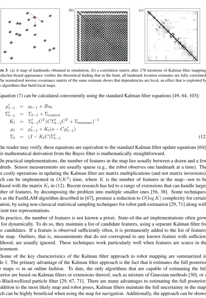
Before discussing the Kalman filter-based mapping algorithm, let us inspect an example. Figure 2 shows an image of a map obtained using the Kalman filter approach (courtesy of Stefan Williams and Hugh Durrant-Whyte [104]). Shown in this image is the path of an underwater vehicle, along with range mea-surements obtained using a pencil sonar. The map itself consist of 14 point features, extracted from the sonar data. Five of those features correspond to thin, vertical artificial landmarks; the other correspond to other reflective objects in the environment. The ellipses around these landmarks illustrate the residual un-certainty that remains after mapping, as specified by the covariance matrix Σ. Similarly, the robot’s path itself is uncertain, as indicated by the ellipses that can be found in regular intervals along the path. All these ellipses, are two-dimensional projections of a single Gaussianhµ,Σithat represents the joint posterior over all landmark locations and the robot pose. Additional dots in Figure 2 depict hypotheses for the location of additional landmarks whose evidence is too weak for them to be included in the map. Figure 3 illus-trates the result after successful mapping, using a simulation example. Of importance is the matrix shown in Figure 3b, which depicts the correlation (normalized covariance matrix Σ) between the robot’s three-dimensional pose and all 20 landmarks’ two-three-dimensional location. The checkerboard appearance suggests that there are strong correlations between all location estimates in the x- andy-dimensions. This makes sense, since measurements convey only information about the relative location of the robot to landmarks (and, by induction, between the landmarks themselves), not about their absolute coordinates. Consequently, the final map in Figure 3a is still somewhat uncertain.
Kalman filter mapping relies on three basic assumptions. First, the next state function (motion model) must be linear with added Gaussian noise. Second, the same characteristics must also apply to the per-ceptual model. And third, the initial uncertainty must be Gaussian. We will now elaborate on these three assumptions.
A linear next state function is one where the robot posest and the mapmtat time tdepend linearly on the previous posest−1 and mapmt−1, and also linearly on the controlut. For the map, this is trivially the case since by assumption, the map does not change. However, the pose st is usually governed by a nonlinear trigonometric function that depends nonlinearly on the previous pose st−1 and the control ut.
Figure 2: Example of Kalman filter estimation of the map and the vehicle pose. Courtesy of Stefan Williams and Hugh Durrant-Whyte of the Australian Centre for Field Robotics at the University of Sydney [104].
To accommodate such nonlinearities, Kalman filters approximate the robot motion model using a linear function obtained via Taylor series expansion. The resulting Kalman filter is known as extended Kalman
filter [64] (see also [47]), and single motion commands are often approximated by a series of much smaller
motion segments, to account for nonlinearities. For most robotic vehicles, such an approximation works well. The result of the linearization is that the state transition function can be written as a linear function with added Gaussian noise:
p(x|u, x0) = Ax0+Bu+εcontrol (10)
HereAandBare matrices that implement linear mappings from statesx0and the motion commanduto the next state variablex, respectively. Noise in perception is modeled via the variableεcontrol, which is assumed
to be normal distributed with zero mean and the covarianceΣcontrol.
As with robot motion, sensor measurements in robotics are usually nonlinear, with non-Gaussian noise. Thus, they are also approximated through a first degree Taylor series expansion. Put into equations, Kalman filter methods require thatp(z|x)withx=hs, miis of the following form:
p(z|x) = Cx+εmeasure (11)
Here C is a matrix (a linear mapping), andεmeasure is normal distributed measurement noise with zero
mean and covarianceΣmeasure. Such approximations are known to work well for robots that can measure
(a) (b) (c)
Figure 3: (a) A map of landmarks obtained in simulation, (b) a correlation matrix after 278 iterations of Kalman filter mapping. The checker-board appearance verifies the theoretical finding that in the limit, all landmark location estimates are fully correlated. (c) The normalized inverse covariance matrix of the same estimate shows that dependencies are local, an effect that is exploited by some algorithms that build local maps.
in Equation (7) can be calculated conveniently using the standard Kalman filter equations [49, 64, 103]:
µ0t−1 = µt−1+But Σ0t−1 = Σt−1+ Σcontrol
Kt = Σ0t−1CT(CΣ0t−1CT + Σmeasure)−1
µt = µ0t−1+Kt(o−Cµ0t−1)
Σt = (I−KtC)Σ0t−1 (12)
As the reader may verify, these equations are equivalent to the standard Kalman filter update equations [64]. Their mathematical derivation from the Bayes filter is mathematically straightforward.
In practical implementations, the number of features in the map lies usually between a dozen and a few hundreds. Sensor measurements are usually sparse (e.g., the robot observes one landmark at a time). The most costly operations in updating the Kalman filter are matrix multiplications (and not matrix inversions), which can be implemented in O(K2) time, where K is the number of features in the map—not to be confused with the matrixKtin (12). Recent research has led to a range of extensions that can handle larger number of features, by decomposing the problem into multiple smaller ones [56, 38]. Some techniques, such as the FastSLAM algorithm described in [67], promise a reduction toO(logK)complexity for certain situation, by using non-classical statistical sampling techniques for robot path estimation [29, 71] along with efficient tree representations.
In practice, the number of features is not known a priori. State-of-the-art implementations often grow this list dynamically. To do so, they maintain a list of candidate features, using a separate Kalman filter for these candidates. If a feature is observed sufficiently often, it is permanently added to the list of features in the map. Outliers, that is, measurements that do not correspond to any known feature with sufficient likelihood, are usually ignored. These techniques work particularly well when features are scarce in the environment.
Some of the key characteristics of the Kalman filter approach to robot mapping are summarized in Table 1. The primary advantage of the Kalman filter approach is the fact that it estimates the full posterior over maps m in an online fashion. To date, the only algorithms that are capable of estimating the full posterior are based on Kalman filters or extensions thereof, such as mixture of Gaussian methods [30], or a Rao-Blackwellized particle filter [29, 67, 71]. There are many advantages to estimating the full posterior: In addition to the most likely map and robot poses, Kalman filters maintain the full uncertainty in the map, which can be highly beneficial when using the map for navigation. Additionally, the approach can be shown to converge with probability one to the true map and robot position, up to a residual uncertainty distribution that largely stems from an initial random drift [73, 26, 27]. As is commonly the case with theoretical results,
(a) (b) (c)
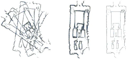
Figure 4: (a) Raw range data of a large hall in a museum. (b) Data aligned with EM using artificial but indistinguishable landmarks. (c) Result of applying the Lu/Milios algorithm to the pre-aligned data.
they only hold under the specific conditions discussed above. They also require that the robot encounters each landmark infinitely often. Nevertheless, this result is the strongest convergence result that presently exists in the context of robotic mapping.
Probably the most important limitation of the Kalman filter approach lies in the Gaussian noise assump-tion. In particular, the assumption that the measurement noiseεmeasuremust be independent and Gaussian
poses a key limitation, with important implications for practical implementations. Consider, for example, an environment with two indistinguishable landmarks. Measuring such a landmark will induce a multimodal distribution over possible robot poses, which is at odds with the (unimodal) Gaussian noise assumption. More generally, Kalman filter approaches are unable to cope with the correspondence problem, which is the problem of associating individual sensor measurements with features in the map.
This limitation has important practical ramifications. Implementations of the Kalman filter approach usually require a sparse set of features which are sufficiently distinctive—either by their sensor characteris-tics or by their location—so that they can be identified reliably. Errors in the identification of environment features usually imply failure of the mapping algorithm. For this reason, Kalman filter approaches are usu-ally forced to ignore large portions of the sensor data, and work with a small number of landmark-type features only. The resulting maps contain the locations of these landmarks but usually lack detailed geomet-ric descriptions of the environment.
A recent extension of the basic paradigm is known as the Lu/Milios algorithm [60]. This algorithm was successfully implemented by Gutmann [39, 41]. The Lu/Milios algorithm is somewhat specific to laser range data. It combines two basic estimation phases: A phase where Kalman filters are used to calculate posteriors over maps, and another where the range measurements in multiple range scans are associated with each other. The correspondence is obtained via maximum likelihood data association, that is, the algorithm simply pairs up nearby measurements. However, by iterating both phases, the correspondence is calculated repeatedly, enabling the approach to recover from wrong correspondences. In practice, this approach is able to build maps from raw data with unknown correspondences. However, the fact that it uses maximum likelihood to ‘guess’ the correspondences—instead of calculating the full posterior over correspondences and maps—imposes important limitations. In practice, the algorithm works amazingly well when the errors in the initial pose estimates are small (e.g., smaller than 2 meters). Larger pose errors,
such as typically encountered when mapping a cyclic environment, cannot be accommodated. Moreover, this approach requires multiple passes through the data, hence is not a real-time algorithm. Figure 4c depicts a map generated using this algorithm from the range data shown in Figure 4b. The final map is highly accurate and exhibits detailed structure. However, the reader should notice that the data fed into this algorithm is pre-aligned. The raw data using the robot’s odometry for pose estimation, shown in Figure 4a, is too erroneous for the Lu/Milios algorithm. The problem with such erroneous data is the failure of the maximum likelihood correspondence step, which in turn leads to wrong maps when using Kalman filtering. This result illustrates the strength and weakness of the basic approach. We note that the pre-alignment from Figure 4a to Figure 4b was performed using an algorithm described in the next section.
The discussion of Kalman filter approaches raises the more general question as to whether it is prin-cipally possible to perform full posterior estimation in the face of unknown correspondences. The basic Kalman filter algorithm cannot cope with ambiguous features, and even extensions such as the Lu/Milios algorithm resort to (brittle) maximum likelihood techniques to guess the best correspondence during map-ping. Unfortunately, calculating the full posterior under unknown correspondences is hard. If there exist
nambiguous features in the world, each measurement of such a feature will in the worst case multiply the modes of the posterior by a factor ofn. Thus, the number of modes in the posterior may grow exponentially over time. This suggests that no incremental algorithm exists that can calculate the full posterior under unknown correspondences. However, recent research suggests that it may suffice to maintain a small num-ber of those modes, using a mixture of Gaussian representation [30] or a—highly related—particle filter representation [67, 71]. Such representations have been applied with great success in lower dimensional robot localization problems [19, 46, 79, 80], commonly under the name multi hypothesis Kalman filters. The development of techniques for posterior estimation with unknown correspondence is currently subject of ongoing research, with enormous potential for practical applications.
6
Expectation Maximization Algorithms
A recent alternative to the Kalman filter paradigm is known as the expectation maximization family of algorithms, or in short, EM. EM is a statistical algorithm that was developed in the context of maximum likelihood (ML) estimation with latent variables, in a influential paper by Dempster, Laird and Rubin [24]. A recent book on this topic illustrates the wealth of research that presently exists on the EM algorithm [65]. Applied to the robotic mapping problem, the EM algorithm has quite orthogonal characteristics. EM algorithms constitute today’s best solutions to the correspondence problem in mapping [11, 101]. In partic-ular, EM algorithms have been found to generate consistent maps of large-scale cyclic environment even if all features look alike and cannot be distinguished perceptually. However, EM algorithms do not retain a full notion of uncertainty. Instead, they perform hill climbing in the space of all maps, in an attempt to find the most likely map. To do so, they have to process the data multiple times. Hence, EM algorithms cannot generate maps incrementally, as is the case for many Kalman filter approaches.
The EM algorithm exploits the chicken-and-egg nature of the mapping problem. In particular, it builds on the insight that determining a map when the robot’s path is known (in expectation) is relatively simple, as is the determination of a probabilistic estimate of the robot’s location for a given map. To exploit this insight, EM iterates two steps: An expectation step or E-step, where the posterior over robot poses is calculated for a given map, and a maximization step or M-step, in which EM calculates the most likely map given these pose expectations. The result is a series of increasingly accurate maps,m[0], m[1], m[2], . . .. The initial map,
m[0], is an empty map.
dtand the robot’s pathst={s1, . . . , st}:
m[i+1] = argmax m Es
t[logp(dt, st|m)|m[i], dt] (13) This equation follows from the Bayes filter under several mild assumptions. The(i+ 1)-th map is obtained from thei-th map by maximization of a log likelihood function. The logarithm is a monotonic function; hence maximizing the logarithm is equivalent to likelihood maximization. Part of the likelihood that is being maximized is the robot’s pathst. However, in mapping the path is unknown. Equation (13), thus, computes the expectation of this likelihood over all possible paths the robot may have taken. Under mild assumptions, (13) can be re-expressed as the following integral:
m[i+1] = argmax m X τ Z p(sτ |m[i], dt) logp(zτ |sτ, m)dsτ (14) Here the right-hand side contains the termp(sτ |m[i], dt), which is the posterior for the posesτconditioned on the datadt and thei-th mapm[i]. Further above, we have already encountered various such estimation problems, and have shown how to use Bayes filters to solve them. The specific problem here is a low-dimensional robot localization problem, since we are given the i-th map and only need to compute the posterior over the robot pose. The key difference to standard localization is that in our case, data in the entire time interval {1, . . . , t} is used to estimate the posterior pose at timeτ, even for τ < t. Thus, we need to incorporate past and future data relative to the time stepτ. Luckily, under further mild assumptions this can be achieved by running Bayes filters twice: once forward in time, and once backwards in time. The forward run provides us with a posteriorp(sτ |m[i], dτ)conditioned on all data leading up to timeτ. The backwards pass gives us the posteriorp(sτ |m[i], dτ+1, . . . , dt)conditioned on all data collected after time stepτ. Multiplication of these two estimates and subsequent normalization gives us indeed the desired probabilityp(sτ |m[i], dt). This calculation is known as the E-step in EM, since it calculates expectations (probabilities) for different poses at all points in time.
The final step, the M-step, is the maximization in (14). Here the expectationsp(sτ |m[i], dt)are fixed, as obtained in the E-step. The goal of the M-step is to find a new mapmthat maximizes the log likelihood of the sensor measurementslogp(zτ |sτ, m), for allτ and all posesstand under the expectation calculated in the E-step. Unfortunately, there exist no known closed form solution to this high-dimensional maximization problem. A common approach is to solve the problem for each map location hx, yi independently [11, 101]. This assumes that the map is represented by a finite number of locations, e.g., by a fine-grained grid. The component-wise maximization is then relatively straightforward. Existing implementations of the EM paradigm rely on grid representations for all densities involved in the estimation process. They also rely on probabilistic maps instead of zero-one maps, which has a smoothing effect on the maximization and avoids getting trapped in local maxima during the optimization.
Key characteristics of the EM algorithm are summarized in Table 1. A key advantage of the EM al-gorithm over Kalman filtering lies in the fact that it solves the correspondence problem. It does so by repeatedly relocalizing the robot relative to the present map in the E-step. The pose posteriors calculated in the E-step correspond to different hypotheses as to where the robot might have been, and hence imply dif-ferent correspondences. By building maps in the M-step, these correspondences are translated into features in the map, which then either get reinforced in the next E-step or gradually disappear.
Figure 5a shows an example of a data set mapped using EM. In this specific example, the robot measures 28 landmarks that are perceptually indistinguishable. These landmarks correspond to corners, intersections and distinctive places; however, for the exercise of mapping with unknown correspondence, the robot is not given any perceptual information that would help disambiguate them. When traversing the large loop in the environment for the first time, the error in the pose estimate using odometry is too large to use it to resolve
(a)
(b)
(c) (d)
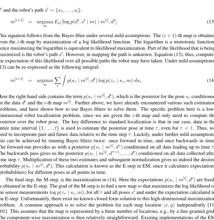
Figure 5: (a) Raw data of a large-scale cyclic environment with indistinguishable landmarks. (b) Occupancy grid map built from raw data using sonar sensors. (c) Map and robot path aligned by EM, demonstrating EM’s ability to solve hard correspondence problems. (d) Occupancy grid map built on top of the outcome of the EM mapping algorithm.
the correspondence problem. Such large loops are known to be challenging to map [40]. Figure 5c shows the result of applying EM to this data set. The resulting map and path is topologically correct. To illustrate the accuracy of the map, Figures 5b and d show occupancy grid maps built from sonar range measurements using the raw range data without and with the poses estimated by EM, respectively.
Such results cannot be obtained using present-day Kalman filtering techniques, since those techniques do not address the correspondence problem in ways that would scale to environments of this complexity. However, we notice that EM is inferior to Kalman filter algorithms in that it is an offline algorithm that is subject to local maxima. Generating maps like the one shown here may take several hours on a low-end PC.
7
Hybrid Approaches
The literature on robotic mapping provides ample examples of hybrid solutions which integrate probabilistic posteriors with computationally more efficient maximum likelihood estimates.
One of the most common approaches, which from a mathematical point of view is inferior to both Kalman filters and EM, is the incremental maximum likelihood method [32, 69, 94, 105, 107]. The basic idea is to incrementally build a single map as the sensor data arrives, but without keeping track of any residual uncertainty. Such a methodology can be viewed as a M-step in EM, without an E-step. The advantage of this paradigm lies in its simplicity, which accounts for its popularity.
Mathematically, the basic idea is to maintain a series of maximum likelihood maps,m∗1, m∗2, . . ., along with a series of maximum likelihood poses s∗1, s∗2, . . .. The t-the map and pose are constructed from the
(a) (b) (c)
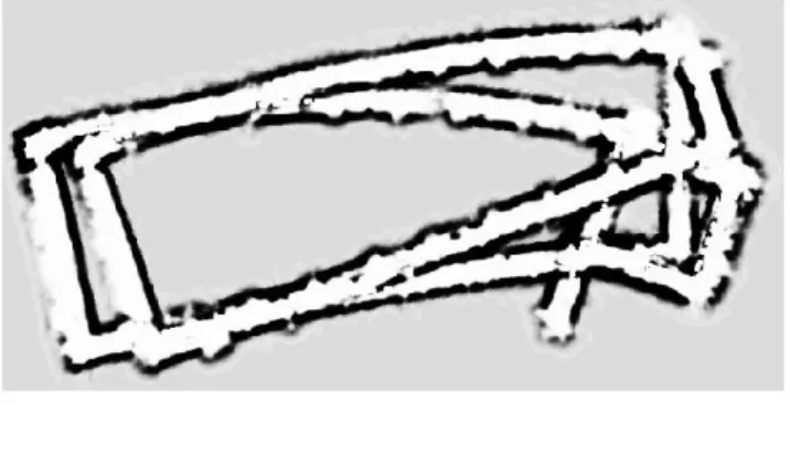
Figure 6: Incremental maximum likelihood mapping: At every time step, the map is grown by finding the most likely continuation. This non-probabilistic approach works well in non-cyclic environment but is generally unable to handle cycles.
(a) (b) (c)
Figure 7: Hybrid approach, which maintains a posterior estimate over the robot poses, represented by a set of particles. When closing the loop, these samples are used to relocalize the robot in the map and correct the map accordingly.
(t−1)-th map and pose via maximization of the marginal likelihood:
hm∗t, s∗ti = argmax mt,st
p(zt|st, mt)p(st, mt|ut, s∗t−1, m∗t−1) (15)
This equation directly follows from the Bayes filter (6) under the assumption that the(t−1)-th map and robot pose are known. In practice, it usually suffices to search in the space of posesst, since the mapmtis usually uniquely determined once the posestis known. Thus, the incremental ML method simply requires search in the space of all posesstwhen a new data item arrives, to determine the poses∗t that maximizes the marginal posterior likelihood. Like Kalman filters, this approach can build maps in real-time, but without maintaining a notion of uncertainty. Like EM, it maximizes likelihood. However, the incremental one-step likelihood maximization differs from the likelihood maximization over an entire data setdt. In particular, once a poses∗t and a mapm∗t have been determined, they are frozen once and forever and cannot be revised based on future data—a key feature of both the Kalman filter and the EM approach.
This weakness manifests itself in the inability to map cyclic environments, where the error in the poses
s∗t may grow without bounds. Figure 6 shows an example where the incremental maximum likelihood approach is used to map a cyclic environment, with a robot equipped with a 2D laser range finder. While the map is reasonably consistent before closing the loop, the large residual error leads to inconsistencies that cannot be resolved by the incremental maximum likelihood approach. This is a general limitation of algorithms that do not consider uncertainty when building maps, and that possess no mechanism to use future data to adjust past decisions.
A B C
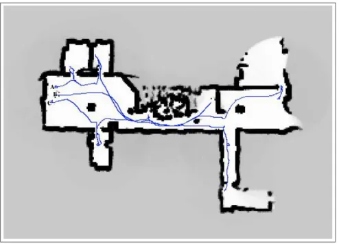
Figure 8: Map built by three autonomously exploring robots. The initial robot poses are on the left as marked by the letters A, B, and C.
mapping, short of the full posterior over maps and poses maintained by Kalman filters. A good example are the algorithms described in [40, 97, 100]. Both of these algorithms use the incremental maximum likelihood approach to build maps, but in addition maintain a posterior distribution over robot posesst. This distribution is calculated using the standard Bayes filter (3) applied to robot posesst(but not maps):
p(st|zt, ut) = η p(zt|st)
Z
p(st|ut, st−1)p(st−1 |zt−1, ut−1)dst−1 (16)
The idea is that by retaining a notion of the robot’s pose uncertainty, conflicts like the one faced by the incremental maximum likelihood method can be identified, and the appropriate corrective action can be taken. Figure 7 shows a sequence of map estimation steps using this approach, for the same data that were used to generate Figure 6. The pose posterior estimatep(st|zt, ut)is implemented using particle filters [22, 28, 57, 77], which is a version of the Bayes filter that represents posteriors by samples. The samples can be seen in all three diagrams in Figure 7. When the robot traverses a cyclic environment, it uses the samples to localize itself relative to the previously built map. When it has determined its pose with high likelihood, it uniformly spreads the resulting error along the cycle in the map. Consequently, the approach still maintains just a single map, which is computationally advantageous. But unlike the incremental maximum likelihood methods, it also has the ability to correct its map backwards in time whenever an inconsistency is detected. Mathematically, this hybrid algorithm can be derived as a rather crude approximation to the EM algorithm, which performs the E-step and the M-step selectively, as discrepancies are detected.
However, the hybrid approach suffers many deficiencies. First and foremost, the decision to change the map backwards in time is a discrete one which, if wrong, can lead to catastrophic failure. Moreover, the approach cannot cope with complex ambiguities, such as the uncertainty that arises when the robot traverses multiple nested cycles. Finally, the hybrid approach is—strictly speaking—not a real-time algorithm, since the time it takes to correct a loop depends on the size of the loop. However, practical implementations appear to work well in real-time when used in office-building type environments.
The hybrid mapping algorithm has been extended to handle multiple robots that jointly acquire a single map [50, 97]. Figure 8 plots a map acquired by three autonomous robots, which coordinated their
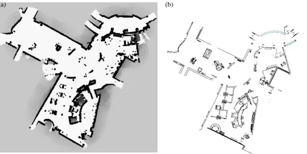
explo-(a) (b)
Figure 9: (a) Occupancy grid map and (b) architectural blueprint of a recently constructed building. The blueprint is less accurate than the map in several locations.
ration efforts while the map was being built [12, 89]. Such results exploit the approximate real-time property of the hybrid algorithm.
8
Occupancy Grid Maps
The mapping algorithms described above all address the mapping problem with unknown robot poses which, as pointed out above, is known as the simultaneous localization and mapping (SLAM) problem. The simpler case—mapping with known poses—has also received attention in the literature. One mapping algorithm, known as occupancy grid maps developed by Elfes and Moravec in the mid-Eighties [32, 69], has enjoyed enormous popularity. This algorithm is used by a number of autonomous robots, typically in combination with one of the algorithms described above.
The central problem addressed by occupancy grid mapping and related algorithm is the problem of generating a consistent metric map from noisy or incomplete sensor data. Even if the robot poses are known, it is sometimes difficult to say whether a place in the environment is occupied or not, due to ambiguities in the sensor data. The best-explored applications of occupancy grid maps require robots with range sensors, such as sonar sensors or laser range finders. Both sensors are characterized by noise. Sonars, in addition, cover an entire cone in space, and from a single sonar measurement it is impossible to say where in the cone the object is. Both sensors are also sensitive to the angle of an object surface relative to the sensor and the reflective properties of the surface (absorption and dispersion).
Occupancy grid maps resolve such problems by generating probabilistic maps. As the name suggests, occupancy grid maps are represented by grids, which are usually two-dimensional [69] but may also cover all three spatial dimensions [70]. The standard occupancy grid mapping algorithm is a version of Bayes filters, just like any other major mapping algorithm. In particular, Bayes filters are used to calculate the posterior over the occupancy of each grid cell. Lethx, yi be the coordinates of a grid cell and mx,y its occupancy. Occupancy is a binary variable: Either the cell is occupied or it is free. The problem, thus, is to calculate a posterior over a set of binary variables, each of which is a single numerical probability
The binary Bayes filter is often written using odds. The odds of an event x with probabilityp(x) is defined as1−p(px()x). In odds notation, the binary Bayes filter for a static maps and with known posesstworks as follows: p(mx,y|zt, st) 1−p(mx,y |zt, st) = p(mx,y |zt, st) 1−p(mx,y |zt, st) 1−p(mx,y) p(mx,y) p(mx,y|zt−1, st−1) 1−p(mx,y|zt−1, st−1) (17) The basic update equation is often implemented in logarithmic form, which is computational advantageous (additions are faster than multiplications) and also avoids numerical instabilities that arise when probabilities are close to zero:
log p(mx,y|z t, st) 1−p(mx,y|zt, st) = log p(mx,y |zt, st) 1−p(mx,y |zt, st) + log1−p(mx,y) p(mx,y) + log p(mx,y |zt−1, st−1) 1−p(mx,y |zt−1, st−1) (18) It is easy to see that the desired probability of occupancy,p(mx,y |zt, st), can be recovered from the log-odds representation. Moreover, we notice that the occupancy grid mapping algorithm is recursive, allowing for incrementally updating the individual grid cells as new sensor data arrives. Finally, occupancy grid maps require two probability densities,p(mx,y |zt, st)andp(mx,y). The latter probabilityp(mx,y)is the prior for occupancy which, if set to 0.5, makes an entire term disappear in Equation (17).
The remaining probabilityp(mx,y|zt, st), is called an inverse sensor model. It specifies the probability that a grid cellmx,yis occupied based on a single sensor measurementzttaken at locationst. The literature has devised numerous versions of this probability, for sensors such as sonars, lasers, cameras (mono and stereo), and infrared sensors [72, 99]. Inverse models for range sensors usually attribute high probability of occupancy for grid cells that overlap with detected range, and low probability for grid cells in between this range and the sensor. These functions can be crafted by hand [69] or learned from sensor data [99].
We already encountered examples of occupancy grid maps in Figures 1a and 5. The maps shown there were built using sonar sensors. Figure 9 gives another example, constructed from laser range finders. In this example, the pose information stwas obtained using the hybrid mapping algorithm described in the previous section. The resulting occupancy grid map exhibits a great level of accuracy when compared with a CAD map of the building, shown on the right.
The occupancy grid mapping algorithm enjoys the reputation of being extremely robust and easy to implement, which has contributed to its popularity. Its major shortcoming is the lack of a method for accommodating pose uncertainty. A second deficiency is inherited from the Bayes filter, which assumes independent noise. When sensor noise is strongly correlated, the resulting maps can be erroneous. This is particularly the case when sonar measurements are integrated while the robot stands still. Most implemen-tations remedy this problem by simply discarding all sensor measurements, unless the robot is in motion. A final, more subtle deficiency stems from the independence assumption between multiple grid cells. Such an assumption, while convenient, can lead to inferior maps. See [96] for more details.
9
Object Maps
Another family of mapping algorithms described in this paper addresses the problem of building maps composed of basic geometric shapes or objects, such as lines, walls, and so on. In mobile robotics, the idea of representing maps by simple geometric shapes can be traced back to a paper by Chatila and Laumond [15], who proposed to represent 2D maps by collection of lines rather than grids. However, they did not provide a
(a) (b)
Figure 10: (a) Polygonal model generated from raw data, not using any geometric shape information. (b) Texture superimposed onto this model.
practical algorithmic solution. Since then, researchers have devised a few practical algorithms that can use object information in the process of mapping, such as [6, 58, 61].
There are four basic advantages of object maps over grid maps: First, object maps can be more compact than occupancy grid maps, especially if the environment is structured. Second, they can also be more accurate, assuming that the basic objects in the approach are adequate to describe the actual objects found in the environment at hand. Third, object representations appear to be necessary for describing dynamic environments where objects might change their location over time. And fourth, object maps are often closer to people’s perception of environments than grid maps, thereby facilitating the interaction between humans and robots. However, object maps also suffer a major disadvantage. In particular, they are usually confined to environments that can be expressed through simple geometric shapes and objects. Real environments are complex, and any list of shapes and objects will typically be incomplete. One way to overcome this limitation is to allow for hybrid maps, which represent some parts of the environment via objects and others using grid map-style representations. Another is to broaden the notion of objects, and learn models of object concurrently to learning the map.
A good example of learning with parametric object models is described in [58, 61]. The specific prob-lem addressed in both of these papers is that of constructing three-dimensional maps. The data used for the mapping task is collected by the robot equipped with two 2D laser range finders. One of those 2D sensors is pointed forward to accomplish localization during mapping. A second sensor is pointed upward perpen-dicular to the robot’s motion direction, enabling the robot to scan the 3D structure of the environment as it moves about the environment. Figure 10 shows a slightly pre-processed raw data set of a 3D structure, represented by small polygons that connect adjacent range measurements. This structure was constructed with the help of the hybrid 2D mapping algorithm described in Section 7, to obtain accurate localization. The surface structure in Figure 10 is extremely rugged, reflecting the noise in the sensor measurements. One might be tempted to apply occupancy grid-style techniques for reducing the noise, as in [70]. However, in this specific data set each feature in the environment is sensed at most once, whereas techniques like occupancy grids require that a grid cell can be measured many times, so that information can be integrated using Bayes filters.
The object mapping approach in [58, 61] remedies this problem by assuming that parts of the environ-ment consists of large flat surfaces—which is the one and only type of object that is accommodated in this approach. This assumption is certainly valid for corridor-like environment with flat walls and ceilings. The technical problem, thus, is how to determine the number, sizes, and locations of these surfaces.
Interestingly enough, this problem can be solved with a variant of the expectation maximization algo-rithm that we already encountered above. EM generates a sequence of object maps that explain the data with increasing accuracym[0], m[1], m[2], . . .. Above, the EM algorithm was used to generate maps, where
(a) Polygonal models generated from raw data
(b) Low-complexity multi-surface model
Figure 11: 3D Model generated (a) from raw sensor data, and (b) using our algorithm, in which 94.6% of all measurements are explained by 7 surfaces. Notice that the model in (b) is much smoother and appears to be more accurate.
the latent variables were robot poses. Here, the poses are known. Instead, the latent variables are corre-spondence variables that specify which of the measurements were caused by which of the flat surfaces—or whether a measurement was caused by a surface at all. For simplicity, let us assume that each measurement
ztis a single range measurement which, by virtue of knowing the robot’s posest, can be mapped into 3D coordinates using the standard geometric laws. Let us assume the world contains J flat surfaces, called
m1, m2, . . . , mJ. For now, let us assumeJ is given, although the work in [58, 61] provides techniques for estimatingJ along the way (see below). The correspondence variables will be written asctjandct∗, where ctjis 1 if and only if a measurementztwas caused by surfacej, andct∗is 1 if and only if this measurement
was not caused by any of the surfaces. The set of all correspondence variables at timetwill be denoted byct, and the correspondences leading up to timetbyct. Clearly, these variables are not observable. However, it turns out that calculating expectations for these correspondence variables for any given mapmis relatively straightforward, as is generating a new improved map under knowledge of these expectations. Thus, the problem lends itself nicely to the EM algorithm.
Applied to this mapping problem, the EM algorithm generates a sequence of maps by maximizing the following expected log likelihood function:
m[i+1] = argmax m
Ect[logp(zt, ct|m, st)|m[i], zt] (19) Notice the similarity to Equation (13). In both cases, EM maximizes a log-likelihood function over the data zt and some hidden variables. In both cases, the hidden variables are integrated out by calculating the expectation over them. However, in the present mapping problem the posesstare known. Instead, the correspondencesctare not.
Under the familiar conditional independence assumptions and further mild assumptions on the nature of sensor noise, this expression unfolds to the following one:
m[i+1] = argmin m X t X j p(ctj |m[i], zt, st) dist(zt, mj) (20)
Here “dist” is the Euclidean distance function, which is obtained by taking the logarithm of a Gaussian noise model. EM maximizes Equation (20) in two steps: The E-step calculates the expectation of the correspon-dence variablesp(cij |m[i], zt, st)andp(ci∗ |m[i], zt, st)for a fixed, given mapm[i]. Put differently, the E-step calculates the probability that a measurementzt was caused by any of the surfaces in the present model. The M-step generates a new mapm[i+1] by maximizing the data log likelihood under these fixed expectations. Both steps are mathematically straightforward and can be implemented in closed form [58]. The result, as stated above, is a sequence of maps that successively maximizes the expected log likelihood of the data or, put differently, generates maps that are increasingly accurate.
The basic algorithm in [58] contains two additional ideas. First, while the EM map itself consists exclu-sively of flat surfaces, the underlying mathematical framework allows for the possibility that measurements are not caused by such surfaces. This makes it possible to include such ‘unexplained’ measurements into the final map, effectively devising a hybrid approach that integrates flat surfaces with raw polygonal models. This property is important when applying any object-based mapping algorithm in practice.
Second, the EM algorithm provides no answer as to how many surfaces are contained in the world. This is not a trivial question, as it is unclear how small a surface we are willing to accept. The approach in [58] solves this through a Bayesian model selection algorithm, which varies the number of surfacesJ in the model concurrently while running EM. The specific approach realizes a Bayesian prior that effectively requires the presence a certain number of measurements in a certain spatial density to warrant the creation of a surface. The algorithm itself is stochastic, seed-starting surfaces at random locations and terminating others whose posterior probabilities, after running EM for a few iterations, do not warrant their existence under the Bayesian prior. The resulting algorithm is a strict maximum likelihood algorithm that generates a single map, which combines large flat surfaces and many small polygons. In a recent paper, the approach was extended as an online algorithm [61].
Figure 11 compares example views, generated without (top row) and with (bottom row) EM and the flat surface model. The object model is 20 times as compact as the original one. In fact, 95% of all original measurements are easily explained byJ = 7flat surfaces. It is also visually much more accurate, due to the fact that the texture is mapped onto a flat surface, instead of a rugged surface like the one shown in Figure 10. The online algorithm described in [61] requires less than two minutes to construct maps of comparable sizes. Clearly, these results are encouraging, though they only hold in cases where the basic geometric object templates describe significant portions of the environment. The remaining challenge is to find richer models that can describe more complex environments than the relatively simple corridor environment.
10
Mapping Dynamic Environments
Physical environments change over time. As noted in Section 3, the vast majority of published algorithm make a static world assumption, hence are principally unable to cope with dynamic environments. Some of these algorithms, however, can be modified to cope with certain types of changes. For example, the Kalman filter approach is easily adapted to one in which landmarks move slowly over time, on trajectories that resemble—for example—Brownian motion. Technically, this is achieved by adding a Gaussian motion variable into the landmark’s location. The effect is an increase in the location uncertainty of each landmark over time, which subsequently may be counteracted by sensing. Such algorithms are popular in the target tracking literature [4, 68, 85]. Similarly, occupancy grid maps may accommodate certain types of motions, by decaying occupancy over time as discussed in [106]. Extensions of occupancy grids exist that can detect frequently-changing locations such as doors [83] and, once detected, quickly estimate their present status during everyday navigation [2]. Nevertheless, the issue of robotic mapping dynamic environments remains poorly explored, and the approaches outlined above cover only a narrow set of cases.

![Figure 2: Example of Kalman filter estimation of the map and the vehicle pose. Courtesy of Stefan Williams and Hugh Durrant- Durrant-Whyte of the Australian Centre for Field Robotics at the University of Sydney [104].](https://thumb-us.123doks.com/thumbv2/123dok_us/1959406.2790113/11.917.148.771.122.615/example-estimation-courtesy-williams-durrant-australian-robotics-university.webp)