scottish institute for research in economics
SIRE DISCUSSION PAPER
SIRE-DP-2010-85
The Distributional Consequences of
Supply-Side Reforms in General Equilibrium
Konstantinos Angelopoulos
Bernardo X. Fernandez
James R. Malley
The Distributional Consequences of
Supply-Side Reforms in General Equilibrium
Konstantinos Angelopoulos, Bernardo X. Fernandez,
James R. Malley
November 2, 2010
Abstract
This paper addresses the issue on whether tax reforms consistent with lower public debt-to-GDP in the long-run can lead to a more e¢ cient and equitable economy. To this end we solve a heterogeneous agent model comprised of a government, a representative capitalist and representative skilled and unskilled workers, under both rational expectations and adaptive learning. Our main …ndings are that (i) reductions in capital taxation, while bene…cial at the aggregate level, lead to increased inequality mainly due to the substitutability of un-skilled labour and capital; (ii) a fall in taxation for un-skilled labour is Pareto improving, which is largely explained by its complementarity with the other factor inputs; (iii) all agents would prefer increasing the tax rate on capital to increasing the tax rate on skilled and un-skilled labour since it leads to relatively lower welfare losses; and (iv) heterogeneity in initial beliefs under adaptive learning quantitatively matters for welfare.
Keywords: tax reform, structural heterogeneity, inequality, adap-tive learning
JEL codes: E25, E62
We would like to thank Apostolis Philippopoulos for helpful comments and sugges-tions. We are also grateful for …nancial support from the ESRC, Grant No. RES-062-23-2292, but the views expressed here are entirely our own. Address for correspondence: Jim Malley, Department of Economics, University of Glasgow, Adam Smith Building, Glasgow G12 8RT. E-mail [email protected].
1
Introduction
There now exists a signi…cant and growing literature on tax reforms in dy-namic general equilibrium (DGE) models, largely focusing on the aggregate welfare bene…ts and the distributional e¤ects of permanent reductions in con-stant capital tax rates. At the aggregate level, studies within a representative agent framework suggest that tax reforms which reduce capital taxation will produce welfare gains for the society, even if the tax burden is concurrently shifted to labour (see e.g. Lucas (1990), Cooley and Hansen (1992) and Gian-nitsarou (2006).1 The aggregate welfare bene…ts from tax reforms that reduce capital taxation are also con…rmed in models with heterogeneous agents (see e.g. Garcia-Mila et. al. (2010)). However, at the same time, heterogeneous agents models make clear that such reforms will have large redistributive ef-fects that will disadvantage di¤erent groups in the society (see e.g. Domeij and Heathcote (2004) and Garcia-Mila et. al. (2010)).2 These results then
suggest that even if they are bene…cial at the aggregate level, tax reforms that reduce capital taxes are not likely to be supported by a majority of the population, unless a compensating mechanism is agreed. It would, of course, be preferable to …nd tax reforms that are Pareto improving since they are more likely to be implemented.
With the above background in mind, this paper aims to welfare-evaluate changes in income tax rates for di¤erent types of agents, to investigate which if any reforms are Pareto improving and if not, which are capable of gener-ating enough gains to compensate potential losers. In most of the literature on tax reforms in heterogeneous agent models, agents di¤er proportionately with respect to their productivity and/or their asset holdings. However, the research by e.g. Stokey (1996) and Krusell et al. (2000) suggests that the roles performed by di¤erent types of labour can be structurally distinct in production. In particular, skilled labour complements capital, whereas un-skilled labour can substitute for capital.3
1At the same time, at the aggregate level, there is also an important literature that
examines optimal tax policy. The general message from Ramsey optimal taxation is that the tax rate on capital should be zero in the long-run (see e.g. Chamley (1986), Chariet al. (1994) and Chari and Kehoe (1999)). This result, however, does not necessarily hold in models incorporating market failures, see e.g. Guo and Lansing (1999), nor in models under time-consistent optimal taxation (see e.g. Kleinet. al. (2008)).
2Studies that take into account the redistributive e¤ects of capital taxation in designing
optimal taxation in heterogeneous agent models are fewer. In Judd (1985), Ramsey-type optimal taxation leads to a zero tax on capital in the long run, but this is not a general result (see e.g. Lansing (1999) and Conesaet. al., (2009)).
3See these papers and the references therein for empirical support regarding these
To achieve our objectives, we build on the research which allows for struc-tural heterogeneity and construct a closed-economy DGE model comprised of three types of private agents and the government. In particular, the model contains a representative capitalist and representative skilled and unskilled workers who all consume output in the product market and supply labour in the factor market in return for labour income. Additionally, the …rst two income groups, subject to intermediation costs, allocate savings to physical capital and government bonds in return for capital income whereas unskilled workers do not save. The representative …rm is owned by the capitalist who hires (skilled and unskilled) labour services and leases physical capital from the factor market for which it pays the competitive wage and interest rate re-spectively. Finally, the government taxes economic activity, provides public spending and issues debt to balance its budget.
We calibrate our model to the UK economy, with the aim of obtaining a realistic assessment of the likely costs and bene…ts of tax reforms for the di¤erent agents. Our modeling permits us to capture key features of hetero-geneity. Following the literature on credit constraints and income inequality (see e.g. Galor and Zeira (1993), Benabou (1996) and Aghion and Howitt (1998)), …nancial intermediation costs allow our model to generate hetero-geneity in savings. In particular, the heterohetero-geneity in savings predicted by our model is consistent with the UK data, which suggest that about 30% of the households in the UK do not save and that the savings of high savers are about …ve times higher than those of low savers. In addition, we use a constant elasticity of substitution (CES) speci…cation, following e.g. Stokey (1996) and Krusell et al. (2000), which assumes di¤erent roles in the pro-duction function for skilled and unskilled labour. This allows our calibrated model to produce factor input elasticities and a wage premium that are in line with empirical studies.
We also relax the assumption of rational expectations, to examine whether bounded rationality in the form of adaptive learning (see e.g. Evans and Honkapohja (2001)), can lead to di¤erent conclusions regarding the welfare costs of tax increases. For instance, Giannitsarou (2006), in a representative agent model, shows that learners can have lower welfare gains from tax re-forms, compared to the case of rational expectations. In the case of bounded rationality, we also consider an additional source of heterogeneity, in the form of the initial beliefs of the agents regarding the equilibrium laws of motion (see e.g. Honkapohja and Mitra (2006), for heterogeneity in learning). In particular, we examine the case where the capitalists are able to predict the rational expectations solution in the post-reform economy and thus use this as their initial guess for the parameters of their policy functions, but the skilled workers cannot and thus use the pre-reform economy to determine
their policy functions in the …rst period after the reform. In other words, for the capitalists the tax reform is perfectly anticipated, while for the skilled workers it is unanticipated. This would correspond to an unequal distribution of information regarding the reform in the economy. As far as we know, this type of heterogeneity has not been considered in the tax reform literature.
As discussed above, we also di¤er from the previous literature on tax reforms in heterogeneous agent models, as we model the complementarities and substitutabilities between the di¤erent types of agents. An additional di¤erence is in the types of tax reform we consider. In particular, in the tax reform literature the main interest has been in policy reforms that lowers the capital tax rate, while increasing the labour tax rate at the same time, to keep the budget balanced (see e.g. Lucas (1990), Domeij and Heathcote (2004) and Garcia-Mila et. al. (2010) and, for the UK, Angelopoulos et al. (2008)). In a heterogeneous agent setup, this implies that cuts in capital taxes will directly hurt the share of the population whose income is primarily from labour, thus suggesting that a large part of the welfare losses of these agents will come from the increased labour taxation. To isolate the e¤ects of changes in each tax rate on all agents, we consider changes in tax rates that are not followed by opposite movements in the other tax rates. Instead, the target for tax reforms is a lower steady-state debt-to-GDP ratio, holding government spending (excluding interest payment on the debt) …xed.
Our proposed analysis is particularly relevant in the current economic en-vironment as economies struggle to deal with aftermath of the world …nancial crisis in 2007/08. Supply-side reforms, aimed at creating a tax system that is more e¢ cient and more equitable, have been on the political and economic agenda for many years.4 Given the burgeoning public debt which has
accu-mulated since the onset of the economic crisis, a number of both demand and supply side measures are being implemented in countries across the world to reduce public debt as a share of national income.5 Indeed in the UK, an
increase in the VAT to 20% together with public spending cuts has been an-nounced. With existing as well as new pressing policy objectives in mind, we employ our modelling framework to address the issue on whether supply-side reforms consistent with lower public debt-to-GDP in the long-run can lead to a more e¢ cient and equitable economy.
Our main …ndings are that (i) reductions in capital taxation, while
ben-4See e.g. the research for the Mirrlees Review, at the Institute for Fiscal Studies for
the UK and the discussion on actual tax reforms in Giannitsarou (2006) and Garcia-Mila
et. al. (2010).
5According to data from the OECD for the G-7 (Economic Outlook 87 database), the
UK, France and the US have experienced the largest percentage increases in debt-to-GDP of 86%, 68% and 58% respectively.
e…cial at the aggregate level, lead to increased inequality mainly due to the substitutability of unskilled labour and capital; (ii) a fall in taxation for skilled labour is Pareto improving, which is largely explained by its comple-mentarity with the other factor inputs; (iii) all agents would prefer increasing the tax rate on capital to increasing the tax rate on skilled and unskilled labour since it leads to relatively lower welfare losses; and (iv) heterogeneity in initial beliefs under adaptive learning quantitatively matters for welfare.
The rest of the paper is organised as follows. Sections 1 through 3 set out the model structure, calibration and steady-state and solution respectively. Section 4 contains the policy analysis and …nally Section 5 concludes.
2
Model
The closed-economy setup which follows describes the interaction of three types of private agents and the government in …nal goods, labour and asset markets.
2.1
Population composition
The population size, N, is exogenous and constant. Among N, Nc < N
are identical capitalists, Ns < N are identical skilled workers, and the rest,
Nu =N Nc Ns, are identical unskilled workers. Capitalists are indexed by
the subscript c= 1;2; :::; Nc, skilled workers by s= 1;2; :::; Ns and unskilled
workers by u = 1;2; :::; Nu. There are also Nf …rms, f = 1;2; :::; Nf. We assume that the number of …rms equals the number of capitalists,Nc =Nf;
and that each capitalist owns one …rm. It is useful, for what follows, to de…ne
Nc=N =nc,Ns=N =ns, Nu=N =nu = 1 nc ns and Nf=N =nf.
2.2
Firms
Each …rm produces a single output, Ytf, using physical capital, Ktf, and labour services. There are two distinct types of labour that are used in the production process, unskilled labour,hfu;t, that can be substituted for capital, and skilled labour,hft, which complements capital.6 The production function is given by a constant returns to scale (CRS) technology assumed to take a constant elasticity of substitution (CES) speci…cation following e.g. Stokey (1996) and Krusell et al. (2000):
Ytf =At
h
Ktf + (1 )hfu;ti hhfti1 (1)
where At is exogenous stochastic productivity; 0< ; (1 ); are the
pro-ductivity of weighted capital and unskilled labor and of skilled labour, re-spectively; 0< <1measures the degree of substitutability between capital and unskilled labour.7
Each …rm acts competitively, taking prices and policy variables as given, and maximises pro…ts given by:
f t Y f t r k tK f t wthft wu;thfu;t (2)
subject to the technology constraint given by (1); where wt and wu;t are,
respectively, the wage rates of skilled and unskilled labour and rkt is the interest rate on capital.8 The di¤erent roles in the production function for
skilled and unskilled labour imply that there will be a skill premium for the former, in the sense that the ratio of wt to wu;t will be larger than unity.
We will calibrate the production function so that the implied factor input elasticities and the resulting wage premium are in line with empirical studies.
2.3
Budget constraints of capitalists
The representative capitalist owns one …rm and receives its pro…ts. He also receives income from providing skilled labour services, hc;t, to the labour
market and income from interest on his accumulated stock of …nancial assets, in the form of capital, Kc;t, and government bonds, Bc;t. The interest rate
on government bonds is given by rb
t. All these sources of income are taxed.
In particular, …nancial asset and pro…t income are taxed at the constant rate
k, while labour income is taxed at the constant rate h.
We assume that those agents holding assets need to pay intermediation or transaction premia due to imperfections in capital markets. For instance, these premia can represent the costs of gathering extra information relating to legal issues, asset-speci…c government regulations, intermediation fees and so on. We follow Persson and Tabellini (1992) and assume a quadratic cost function such that the capitalist incurs a cost of 'k
cKc;t2 for holding physical
capital and of 'b
cBc;t2 for holding government bonds, where 'bc; 'kc > 0
mea-sures the size of the transaction costs.9 The presence of this capital market imperfection and of the associated transaction costs help the model to cap-ture a feacap-ture of realism. However, their main contribution here is that they
7Note that when = 1, unskilled labour serves no purpose in production and the
production function is of the standard Cobb-Douglas form in capital and skilled labour.
8Note that, in equilibrium, pro…ts, f
t, are driven to zero due to perfect competition.
9See also Benigno (2009) for intermediation or transaction costs of the form assumed
will allow us, as we shall see below, to capture household heterogeneity in asset holdings.10
The capitalist uses his income for consumption,Cc;t, investment in capital,
Ic;t, and investment in government bonds, Dc;t. He also receives average
(per agent) transfers from the government, Gt(=Gt=N). Thus, his budget
constraint is:
Cc;t+Ic;t+Dc;t= 1 k rtkKc;t+rtbBc;t +
+ 1 k f
t + 1 h wthc;t+Gt 'bcBc;t2 'kcKc;t2
(3) while the evolution of the stock of capital and government bonds, respectively, are given by:
Kc;t+1 = (1 )Kc;t+Ic;t (4)
Bc;t+1 =Bc;t+Dc;t (5)
where 0< <1is a depreciation rate and Kc;0; Bc;0 >0 are given.
2.4
Budget constraints of skilled workers
The problem of the skilled worker is similar to the capitalist’s, in that he provides skilled labour to the factor market, invests the share of his income he does not consume in capital and government bonds, earns interest rate income on his …nancial stock and pays the same tax rates as the capitalist for these economic activities.
The skilled worker di¤ers, however, in that he pays potentially di¤erent transaction costs, so that the capital market imperfections a¤ect him to a greater extent.11 In particular, we assume that …rm ownership gives an
in-sider advantage in …nancial transactions to the capitalist (due, for instance, to past experience, socioeconomic background, networks, etc.) and thus the size of the transaction costs is lower for the capitalist. The idea that capital mar-ket imperfections can explain heterogeneity has been extensively examined in the income inequality literature (see e.g. Galor and Zeira (1993), Ben-abou (1996) and Aghion and Howitt (1998)). Most of these models assume, for simplicity, that the intermediation cost is either in…nite for some agents (and thus these agents are e¤ectively excluded from the …nancial market) or zero. In this paper, we examine the case of non-zero, …nite intermediation costs for both capitalists and skilled workers where 'bc < 'bs, 'kc < 'ks. We
10Transaction costs also helps to di¤erentiate the Euler conditions for bonds and capital
in the steady-state, thus allowing for a unique solution.
11The skilled worker also di¤ers from the capitalist in that he does not appropriate the
pro…ts of the …rm. Given that, in this model, these pro…ts are zero, in equilibrium, this di¤erence is of course trivial.
di¤erentiate the skilled worker and capitalist even further by assuming that the former has lower initial holdings of capital and government bonds, i.e.
Ks;0 < Kc;0, Bs;0 < Bc;0:12
Accordingly, the budget constraints and the evolution equations for cap-ital and government bonds for the sth skilled worker are:
Cs;t+Is;t+Ds;t = 1 k rktKs;t+rtbBs;t + + 1 h w ths;t+Gt 'bsBs;t2 'ksKs;t2 (6) Is;t=Ks;t+1 (1 )Ks;t (7) Ds;t =Bs;t+1 Bs;t: (8)
2.5
Budget constraint of unskilled workers
Unskilled workers di¤er from capitalists and skilled workers in two important respects. First, they start with zero initial holdings of assets and capital mar-ket imperfections result in them being excluded from the …nancial marmar-kets as in the models of Benabou (1996) and Aghion and Howitt (1998). In the context of the formulation used above, this implies an in…nite intermediation cost.13 Second, we assume that exclusion from capital markets does not
al-low them to acquire the skills to provide skilled labour services, so that their labour e¤ort di¤ers, in nature, from the labour e¤ort of the other two types of agents. Evidence from the UK, introduced later, suggests that skill acqui-sition, in the form of University education, is indeed related to socioeconomic income group.
Thus, the budget constraint of theuth unskilled worker is:
Cu;t = (1 u)wu;thu;t +Gt (9)
where0 u <1is the tax rate on unskilled labour,hu;t is the labour supply
and Cu;t is the consumption.
2.6
Utility function of agents
Each type of householdi=c; s; umaximises:
E0 1 P t=0 tu(C i;t; hi;t) (10)
12For the policy experiments that we conduct, the initial conditions for each agent will
e¤ectively correspond to the steady-state of the pre-reform economy.
13See e.g. Aghionet al. (1999) for a microeconomic rationalisation of credit constraints
subject to the relevant budget constraints given above; whereE0 is the
con-ditional expectations operator.
We use the instantaneous utility function:
ui;t = (Ci;t; hj;t) =
(Ci;t) (1 hi;t)
1 1
1 (11)
where 0 < ;1 < 0 are the weights attached to each argument of the utility function and >1 is the coe¢ cient of relative risk aversion.
2.7
Government budget constraint
Following the literature on tax reforms (see e.g. Lucas (1990), Cooley and Hansen (1992), Giannitsarou (2006) and Garcia-Milà et al. (2010)), we do not model government spending.14 Instead, government expenditure takes
the form of transfers to the private agents, Gt. To …nance these, it taxes
income from labour and …nancial assets and issues government bonds, Bt.
The budget constraint of the government is thus given by:
Gt+ 1 +rtb Bt=Bt+1+Nc[ k rktKc;t+rbtBc;t + hwthc;t]+
+Ns[ k rtkKs;t+rbtBs;t + hwths;t] +Nu[ uwu;thu;t]. (12)
2.8
Market-clearing conditions
The market clearing conditions for the capital, bond, skilled and unskilled labour and product markets respectively are:
NfKtf =NcKc;t+NsKs;t (13) Bt=NcBc;t+NsBs;t (14) Nfhft =Nchc;t+Nshs;t (15) Nfhfu;t =Nuhu;t (16) NfYtf =NcCc;t+NsCs;t+NuCu;t+Nc[Kc;t+1 (1 )Kc;t] + (17) +Ns[Ks;t+1 (1 )Ks;t] +Nc 'bcB 2 c;t+' k cK 2 c;t +N s 'b sB 2 s;t+' k sK 2 s;t ,
where (17) gives the aggregate resource constraint of the economy.
14To address distributional e¤ects of spending reforms, the possible bene…ts of public
spending for di¤erent socioeconomic groups would need to be added to our model. More-over, the potential distorting or crowding-out e¤ects of public spending would also need to be more realistically incorporated to capture the e¤ects of increased spending on the interest rate over and above changes to the marginal product of capital.
2.9
Decentralised competitive equilibrium
The decentralised competitive equilibrium (DCE) is de…ned when (i) house-holds and …rms optimize, taking prices and policy as given; (ii) all constraints are satis…ed; and (iii) all markets clear. The optimality conditions for the heterogenous households include four from the capitalist and four from the skilled worker and two from the unskilled worker. In particular, each repre-sentative capitalist and skilled worker chooses fCc;t; hc;t; Kc;t+1; Bc;t+1g1t=0 to
maximise discounted lifetime utility subject to (3 5) and fCs;t; hs;t; Ks;t+1; Bs;t+1g1t=0 subject to (6 8), respectively. Whereas the representative
un-skilled worker chooses fCu;t; hu;tg1t=0 subject to (9). Finally, each
represen-tative …rm chooses nKtf; hfu;t; hfto1
t=0 to maximises pro…ts subject to the
technology constraint (1). In addition to these thirteen …rst-order condi-tions, the DCE also includes the production function (1), two of the three budget constraints from the households’ problems, the government bud-get constraint (12), the market clearing conditions (13)-(16) and the ag-gregate resource constraint (17). We substitute out the Lagrangian mul-tipliers and output, using the appropriate …rst-order conditions and the production function, respectively, and use the market clearing conditions (13)-(16) to substitute out Ktf; hfu;t; hft and Bt. We can then summarise the
DCE by a system of fourteen equations in the paths of the following vari-ables: (Cc;t; Cs;t; Cu;t; hc;t; hs;t; hu;t; wt; wu;t; Kc;t+1; Ks;t+1; Bc;t+1; Bs;t+1; rkt; rbt)
given the exogenously set stationary AR processes for technology and …s-cal policy instruments which are discussed below.15 We de…ne the
rele-vant aggregate, economy-wide quantities using a capital letter Xt, for Xt = fCt; It; Kt; Bt; Ytg.
2.10
The motion of productivity and …scal policy
in-struments
2.10.1 Total factor productivity
Following the literature, we assume that the stochastic process determining
At is an exponential …rst-order Markov process:
At=A (1 a) 0 A a t 1e "t (18)
where A0 >0 is a constant, 0< a <1 is the autoregressive parameter and
"t iid(0; 2) are random shocks to productivity.
15To save space we have not reported the 14-equation DCE system here but it will be
2.10.2 Policy instruments
Given that we wish to analyse the welfare implications of permanent tax regime changes, all tax rates are treated as exogenous constants,0 k; h; u
<1. In particular, in the policy reforms that we will examine, the economy will start from the steady-state and will be subjected to an exogenous, per-manent change in one or more tax instruments, holding the other policy in-struments, including G, constant at the pre-reform steady-state values. We examine economic outcomes and welfare in the new steady and during the transition period to the new steady-state. While we do not analyse the wel-fare implications of changes in government spending, the calibrated value of
G
Y is important in helping to obtain the current steady-state debt-to-output
ratio for the UK.
3
Calibration and steady-state
In Table 1 below, we next calibrate the structural parameters of the model so that its steady-state solution reported in Table 2 re‡ects the main empirical characteristics of the UK economy. The calibration also provides empirical justi…cation for the key modelling decisions made above.
3.1
Distinguishing agent types
3.1.1 Population shares
We …rst wish to map out agent heterogeneity and thus distinguish the three types of households by their di¤ering shares in the population, ni. According
to the Family Resources Survey in 2008-2009, 28%of households do not have any savings, 53% have savings up to £ 20,000 and 19% have savings above £ 20,000.16 In light of this, since we assume that unskilled workers do not
have savings, we set nu equal to 30%. At the other end of the distribution, since we model capitalists as the income group with the highest share of savings and assets, we set nc to 20% implying that ns is 50%. Other data
providing an additional dimension by which unskilled workers di¤er from skilled workers and capitalists is that the former group o¤ers a labour input that is lacking in skills. According to the Labour Force Survey, O¢ ce for National Statistics17, in 2003, 28% of the working population was employed in semi-routine and routine occupations, whereas the remaining share worked
16The Survey is sponsored by the Department for Work and Pensions (see Table 4.9 for
the information reported here).
in supervisory, technical, professional and managerial occupations, which require an increasingly higher skilled labour input. Moreover, according to data from the Department for Education and Skills on the participation rates in higher education for di¤erent income groups, the participation ratio was about three times higher in the 1990s for the three highest, relative to the three lowest groups.18 Thus, there appears to be adequate support for
associating skill with income group.
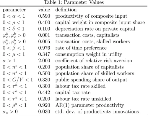
Table 1: Parameter Values parameter value de…nition
0< <1 0.590 productivity of composite input
0< <1 0.400 capital weight in composite input share
0 1 0.100 depreciation rate on private capital
'kc; 'bc >0 0.001 transaction costs, capitalists
'k
s; 'bs>0 0.005 transaction costs, skilled workers
0< <1 0.976 rate of time preference
0< <1 0.347 consumption weight in utility
>1 2.000 coe¢ cient of relative risk aversion
0< nc <1 0.200 population share of capitalists
0< ns <1 0.500 population share of skilled workers
0< G=Y <1 0.330 public spending share of output
0< h <1 0.300 labour tax rate skilled
0< k <1 0.442 capital tax rate
0< u <1 0.200 labour tax rate unskilled
0< a<1 0.920 AR(1) parameter productivity a>0 0.030 std. dev. of productivity innovations
3.1.2 Asset holdings
We next turn to heterogeneity in asset holdings and returns to labour which governs the choice of the relevant production parameters. In particular, following e.g. Stokey (1996), we set the productivity of the composite input in the production function, to 0:59 and , the weight of capital in the composite input share to 0:4. This implies that, at the steady-state, the capital to skilled labour elasticity of substitution is 0:67, the elasticity of capital with respect to unskilled labour is 0:88 and the elasticity of skilled to unskilled labour is 1:30. These elasticities are well within the range of estimated elasticities of substitution in the literature (see e.g. Krusell et al. (2000) for a review of such studies). In turn, these parameters and the implied elasticities lead to a steady-state skill premium, de…ned as log
di¤erences between the wage rates for skilled and unskilled labour, of 24%. Also note that the ratio of the wage rates for skilled and unskilled labour is
1:28. These values are again broadly consistent with estimates for both the UK and the USA. For the UK, Walker and Zhu (2008) estimate a college premium (in log di¤erences) of about 18% for males and 28% for females. Machin (1996) computes the ratio of wages between non-manual and manual jobs in manufacturing that ranges between 1:3 and 1:5, from 1970 to 1990. For the USA, Krusell et al. (2000) report a college premium, in terms of wage ratios, of about 1:18 in 1990.
3.1.3 Savings
Heterogeneity in savings is controlled for, as explained in the previous section, by the parameters that govern transaction costs in the …nancial markets. In particular, following the models in e.g. Galor and Zeira (1993), Benabou (1996) and Aghion and Howitt (1998), we set these costs to in…nity for the unskilled workers, which implies that these agents do not have any savings. As said above, about28% of the UK households do not save. Regarding the households with positive savings, data from the Family Resources Survey of 2008-2009 suggest that households in the highest saving bracket have …ve times higher savings than the other savers, on average. In terms of our model, this di¤erence is applied to the representative capitalist and skilled worker by setting the transaction costs for the latter to be …ve times greater than the former. For simplicity, we set this cost in capital asset markets to be the same in the bond market. We chose the level of the transaction costs parameter, so that in combination with a usual annual depreciation rate, , of10%, the total ratio of capital to GDP in the steady-state is about2, which again coheres with UK data.
3.1.4 E¤ective tax rates
E¤ective average tax rates for capital and labour income are constructed by following the approach in Conesa et al. (2007).19 We use data from the National Accounts and the Public Sector, Taxation and Market Regulation databases (available from OECD.Stat), to obtain the same series as in Conesa
et al. (2007) for 1970-2005.20 The average capital tax rate over the time period is k = 0:442, while the average labour income rate is 0:27. Using
19See their Appendix B for more details.
20As an alternative, we have also used the ECFIN e¤ective average tax rates (see
Martinez-Mongay (2000)). Both approaches give similar long-run averages of labour tax rates, while the ECFIN capital tax rate is higher.
data from Social Trends 38, O¢ ce for National Statistics, we are able to approximate the progressivity of the UK income tax system at about 1:6.21 A
ratio of h= u = 1:6, together with the requirement that the weighted average
of the two tax rates equal the e¤ective labour income tax rate, would imply that h = 0:304and u = 0:19. However, the progressivity of income taxation
probably overestimates the progressivity of labour income taxation, which is our interest here. This is because, in light of the data discussed, we would expect the higher income brackets to have more capital income compared to lower income brackets. On the other hand, the lower the progressivity ratio, the higher the implied value of u. We thus use a progressivity ratio
of h= u = 1:5 for the calibration, which guarantees that u is equal to the
base income tax rate. Accordingly, we approximate the lower tax rate, u,
at 20%, and the higher labour income tax rate, h at30%.
3.2
Parameters common to all agents
We next approximate the rate of time preference, , so that1= is equal to 1 plus the ex-post real interest rate, where we use real interest rate data from OECD Main Economic Indicators, from 1970-2005. This gives a value 0:976
for . Following Kydland (1995), we set , the weight given to consumption relative to leisure in the utility function, equal to the average value of work versus leisure time, which is obtained using data on hours worked from the OECD Economic Outlook database, from 1970-2005.22 We also use a com-mon value from the literature for the intertemporal elasticity of consumption,
1= = 0:5or = 2.
Given that we will evaluate policies that reduce the debt-to-GDP ratio below, we calibrate the share of government spending in GDP,G=Y, to obtain aB=Y ratio of70%based on o¢ cial forecasts for 2011-2013 (see e.g. the Pre-Budget Forecast, June 2010, O¢ ce for Pre-Budget Responsibility)23. Finally, the
AR(1) relation for the productivity process in (18) is estimated using TFP data from the O¢ ce for National Statistics, 1970-2005. The estimated values for a is 0:92and is signi…cant at less than the 1% level of signi…cance. The standard deviation, a, is 0:03.
21This is obtained by calculating the average income tax rate that applies approximately
to the lower30%and the upper70%of the tax payers. We then add the national insurance contribution rate of11% and calculate the ratio of these two e¤ective average tax rates.
22To obtain this we divide total hours worked by total hours available for work or leisure,
following Ho and Jorgenson (2001). They assume that there are 14 hours available for work or leisure per day with the remaining 10 hours accounted for by physiological needs.
3.3
Steady-state
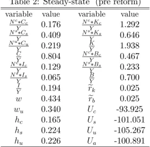
The steady-state solution of the model in this, pre-reform, high debt equi-librium, is given in Table 2 below in terms of the aggregate variables. In particular, we see that the capitalists consume in total17:6%of total income (or about 22% of total consumption24), skilled workers consume in total
40:9% of total income (or around 51% of total consumption) and unskilled workers consume in total 21:9% of total income (or approximately 27% of total consumption). In addition, the capitalists in total have around 67% of total savings and own about67% of the capital and government bonds in the economy. As said above, the ratio of savings, Ic=Is, and assets, Kc=Ks and
Bc=Bs, of the representative capitalist to the representative skilled worker,
are equal to …ve. Note also that the net (after depreciation, tax and trans-action costs) interest rates on capital and bonds, are given respectively by:
e rk=rk(1 k) 2'kc nc nc +ns Kc 2' k s ns nc+ns Ks (19) e rb =rb(1 k) 2'bc nc nc+ns Bc 2' b s ns nc+ns Bs (20)
and are equal in the steady-state.
It is also worth noting that the labour supply elasticities of this model are more in line with microeconometric studies than in the standard aggregate RBC models. In particular, the Frisch (or -constant) labour supply elastic-ity (see e.g. Browning et. al., 1999) is 3:41 for capitalists, 0:43 for skilled and 2:31for unskilled workers. Microeconometric studies (see e.g. Browning
et. al. (1999) for a review) generally suggest that the Frisch labour supply elasticity is less than one and the standard RBC model implies an elasticity around four (see e.g. King and Rebelo, (1999)). The elasticities reported here suggest that capitalists (skilled workers) are less (more) dependent on labour income respectively.
24This is calculated as (Nc C c)=Y
C=Y = (N c C
c)=C. The same formula is used below for
Table 2: Steady-state (pre reform)
variable value variable value
Nc C c Y 0.176 Nc K c Y 1.292 Ns Cs Y 0.409 Ns Ks Y 0.646 Nu C u Y 0.219 K Y 1.938 C Y 0.804 Nc B c Y 0.467 Nc I c Y 0.129 Ns B s Y 0.233 Ns Is Y 0.065 B Y 0.700 I Y 0.194 erk 0.025 w 0.434 erb 0.025 wu 0.340 Uc -93.925 hc 0.165 Us -101.051 hs 0.224 Uu -105.267 hu 0.226 Ua -100.891
The skill premium, measured as the log di¤erences in the wage rates is about24%as noted earlier. In the steady-state, capitalists work considerably less than skilled and unskilled workers, who work more or less the same time (see the hi …gures in Table 2). Also note that in the steady-state Cc =
0:1349; Cs = 0:1253 and Cu = 0:1120. Thus in terms of welfare, Ui, higher
consumption and lower work e¤ort make the capitalists better o¤, followed by the skilled and unskilled workers respectively. The weighted average measure of aggregate or Benthamite lifetime utility, Ua, is also reported in Table 2.25
4
Model Solution
To solve the model, we start by taking the …rst-order Taylor series ex-pansion of the DCE and exogenous process for productivity around their respective steady-states. For any variable Xt, these values are denoted
b
Xt= logXt logX. We next re-express the model in matrix form as
second-order di¤erence equation system:
xt=M1Etxt+1+M2xt 1 +M3zt
yt=N1xt+N2xt 1+N3zt+N4Etxt+1
zt= zt 1+ut:
(21)
25The lifetime utility of agent i in the steady-state is given by U
i = (1
T
) 1 ui, for
i = c; s; u, where ui is the welfare of i calculated at the steady state using (11) and
wherext = h
^
Bc;t+1;K^c;t+1;B^s;t+1;K^s;t+1
i0
contains the endogenous state vari-ables; yt =
h
^
Cc;t;C^s;t;C^u;t;^hc;t;^hs;t;h^u;t;^rtb;r^kt;w^t;w^u;t
i0
the endogenous con-trol variables; andzt= [^at+1]the exogenous state variables.26 The variousM
and Nmatrices contain convolutions of the structural parameters calibrated in Table 1. Finally, since we only have one exogenous state variable, = a
and ut="t+1.
In what follows we use (21) to brie‡y describe how we obtain both the rational expectations (RE) and adaptive learning (AL) solutions of the log-linearised model. Since these methods are well known, our purpose is merely to set out notation and variable de…nitions which will be used in the results and analysis below.
4.1
Rational expectations
Employing the undetermined coe¢ cients method, agents …rst guess that the equilibrium laws of motion for the state variables under RE have the following linear form:
xt= xxt 1+ zzt (22)
where x and z are coe¢ cient matrices. Substituting for zt using the last
equation in(21) gives:
xt= xxt 1+ zzt 1+ z 1
ut (23)
where x = x and z = z . Leading (23) by one-period and taking
expectations of both sides yields:
Etxt+1 = xxt+ z zt (24)
since z 1E
t[ut+1] = 0. Substituting (24) and (23) into the …rst equation
of (21) gives: xt = (I M1 x) 1M 2 xt 1+ + (I M1 x) 1( M1 z+M3) zt 1+ut : (25)
Comparing(25)with(23)implies that the unique RE solution of the reduced-form model is given by the two parameter matrices, hereafter denoted by x
and z, that satisfy the following two equations:
x = (I M1 x) 1M2
z= (I M1 x) 1(M1 z+M3) : (26)
26For examples of others papers in the literature using this particular reduced form, see
Evans and Hokhaponja (2001), Kasa (2004), Giannitsarou (2006) and Carceles Poveda and Giannitsarou (2008).
Assuming x and z exist, the solution for the model’s state variables under RE is:27
xt = xxt 1+ 1 zzt: (27)
Substituting(27) and the expected value of its lead into the second equation of (21) gives the RE solution for the model’s control variables:
yt = h N1 x+N2+N4 2 x i xt 1+ + N1 1 z+N3+N4 z+ x 1 z zt: (28)
4.2
Adaptive learning
Under the AL hypothesis, it is also assumed that private agents can correctly guess the form of the equilibrium policy functions of the state variables given by (22). However, in contrast to the RE solution, it is assumed that they do not know the time-invariant parameter values given by x and z, which ultimately govern the dynamics of the economy.28 Therefore, they must rely
on past data and a recursive learning algorithm to estimate these parameters to produce forecasts of the endogenous state variables for the next period. As new data become available in each period, they revise their parameter estimates so that their forecasting errors are corrected gradually.
More formally, agents’ expectations are assumed to follow a so-called perceived law of motion (PLM) of the form:
Etxt+1= ~x;t 1xt+~z;t 1zt (29)
where parameters ~x and ~z are the estimates of x and z coming from
a recursive least-squares regression andE denotes that expectations do not follow the RE hypothesis.29
Following a similar procedure as under RE, we substitute (29) into the …rst equation of (21) to obtain:
xt=P1xt 1+ 1P2zt (30)
27The two solution matrices
x and z, were obtained applying the method proposed
by Klein (2000).
28Adaptive learning has its foundations in the work of Marcet and Sargent (1989) and
Evans and Honkapohja (2001).
29Note, we follow the common assumption (see, e.g. Evans and Honkaphoja (2001) and
Carceles-Poveda and Giannitsarou (2007)) that at periodt agents form expectations for
xt+1 using their estimates from the previous period, ~x;t 1 and ~z;t 1, which allows us to avoid a problem of simultaneity in the learning process.
where P1= (I M1~x;t 1) 1 M2 P2= (I M1~x;t 1) 1 M1~z;t 1+M3 : (31) Equation (30) is referred to as the actual law of motion (ALM) since every new observed value ofxtdepends on the deep parameters of the model
econ-omy but also on the agents’forecasts given by the PLM (29).
The actual laws of motion for the control variables under learning are found by substituting (30) for xt and (29) for Etxt+1 in the second equation
of (21) giving: yt = h N1P1+N2 +N4~x;t 1P1 i xt 1+ + h N1 1P2+N3+N4 ~x;t 1 1 P2+~z;t 1 i zt: (32)
4.2.1 Recursive least-squares learning
We next focus on how the estimates ~x and ~z in (29) are obtained. We …rst de…ne a vector wt containing the observed values of all the state
vari-ables (including the exogenous process) and another vector ~t = [~x;t;~z;t]0
containing the parameter estimates obtained in each period.30 In what
fol-lows, we will assume that all agents who form expectations, namely capi-talists and skilled workers, follow a recursive least-squares (RLS) learning algorithm. According to this algorithm (see e.g. Evans and Honkapohja (2001) and Carceles-Poveda and Giannitsarou (2007)), in each period agents estimate the parameter matrices ~t = [~x;t;~z;t]0 as they try to …nd their
corresponding true values = [ x; z]0 which come from the RE solution.
For this purpose they make use of all the available data up to that period in a least-squares regression:
xt= ~ 0
wt 1+et (33)
to get a new estimate~t, whereetis the forecast error. According to the
least-squares method,~twill be the coe¢ cient vector which minimizes PT t=1e 2 t and is given by: ~ t= T X i=1 wi 1w 0 i 1 ! 1 T X i=1 wi 1x0i (34)
30Note that under our model setup we havew
The estimator above can be written in a recursive fashion for t= 1;2;3:::, as follows: ~ t= ~t 1+gtRt1wt 1(xt ~ 0 t 1wt 1)0 Rt=Rt 1+gt wt 1w 0 t 1 Rt 1 (35) where Rt is a matrix with the second moments of the regressors included in
wt; (xt ~ 0
t 1wt 1) is the latest forecast error that will be used to correct
the current estimates; and gt = 1=t is the gain sequence implying that as t
increases, every new forecast error will have a lower relative importance.31
4.2.2 Stability and convergence
An important issue is whether the learning algorithm will converge to the RE solution. We …rst consider the so-called expectational stability or E-stability of the model under AL (see the Appendix for further details). Intuitively, the RE solution = [ x; z]0 will be E-stable under learning if small deviations
from it return to = [ x; z]0 under the chosen learning rule. For our model, the E-stability condition is met for the base calibration and all policy experiments considered below.
A second condition for convergence is the stationarity of the RE solution. This requires that the eigenvalues of xhave real parts less than one, ensuring that the part of the RE solution associated with the lags of the state variables do not have an explosive path. The stationarity condition is also met for the base calibration and all policy experiments considered below.
Evans and Honkapohja (2001) show that if the E-stability and stationarity conditions are satis…ed, the RLS algorithm converges locally to x and z
and thus the model at hand is learnable. Honkapohja and Mitra (2006) show that the above conditions also guarantee local convergence in models with structural heterogeneity and heterogeneous initial beliefs. However, these two conditions cannot ensure global convergence of the learning algorithm to the RE solution. As we shall see below, for two of our experiments, where we initialise learning from a point that is far from the RE solution, the learning algorithm breaks down as it implies that the adaptive learners make such big mistakes that a well de…ned solution to the problem cannot be obtained. In other words, the RE solution is not learnable in these cases.
31We make use of Matlab functions made available by Carceles-Poveda and Giannitsarou
5
Policy analysis
5.1
La¤er curves in tax revenue and debt
Our aim is to evaluate the e¤ects of tax reforms that are consistent with a particular long-run debt-to-output target, both at the aggregate level but also for each heterogeneous group of agents in the population. To this end, we …rst calculate the change in a tax rate (or a combination of tax rates) required to bring the debt-to-GDP ratio to a desired level at the steady-state, leaving all the other tax rates and parameters in the model constant. In particular, we start from the current (or pre-reform) steady-state in the economy and calculate the new (or post-reform) steady-state, where the debt-to-GDP ratio is given at the 60% target and a tax rate (or a combination of tax rates) is chosen to satisfy the government budget constraint.
The relationship between the tax revenue from a particular tax base and the associated tax rate is, in general, given by a La¤er curve (see e.g. Schmitt-Grohé and Uribe (1997) for a discussion of La¤er curves in tax revenue in a DGE context). Thus, in our model, an increase (decrease) in a tax rate can lead to either increases (decreases) or decreases (increases) in the tax revenue collected from this tax base, depending on whether the economy is on the upward or downward slopping part of the curve, respectively. In a heterogenous agent context, the complementarity/substitutability of the factors in the production function implies that a tax rate change will have spillover e¤ects to the tax revenue collected from the other tax bases. For instance, an increase in the capital tax rate will decrease the capital supply, but will tend to increase the supply of unskilled labour, which can substitute for capital in production. Thus, the tax revenue collected from the tax base of unskilled labour income is likely to increase after an increase in the capital tax. Hence, these spillover e¤ects, due to the form of technology employed, imply that the relationship between total tax revenue and the tax rates can be di¤erent from the relationship between tax revenue from a particular tax base and the tax rate. In particular, the economy can be on one side of the La¤er curve of tax revenue from a particular tax base but on either side the total revenue La¤er curve.
A lower level of debt in the steady-state implies that there will also be a reduction in interest payments on debt and thus in total government spend-ing, assumspend-ing, as we do here, that the remaining components of government spending do not change. Hence, tax reforms consistent with reducing steady-state debt will need to generate a lower level of total tax revenue.32 As long
32This is di¤erent from the analysis in e.g. Lucas (1990), Angelopoulos et al. (2008)
as a La¤er curve exists in tax revenue with respect to the tax rates, these tax changes can take the form of either decreases or increases in the tax rates since this relationship suggests that a particular tax revenue target can be achieved by two tax rates. We would then expect that there should be a Laf-fer curve characterising the relationship between debt and debt-to-GDP with respect to the tax rates. We plot and discuss these relationships below.33
The above discussion implies that, consistent with the analysis in Schmitt-Grohé and Uribe (1997), for a given level of debt, when a tax rate is the variable that is chosen to satisfy the government budget constraint, it can have two long-run solutions.34 A critical condition for this is that there
is a La¤er curve with respect to total tax revenue. As will be discussed below, the role of the complementarity/substitutability in the capital and labour supply policies of the heterogeneous agents is important in obtaining this La¤er curve and thus in making both long-run solutions empirically plausible. In addition, this complementarity/substitutability implies that the optimal reactions to tax reforms will have distributional e¤ects that might di¤er between the two long-run solutions, across the di¤erent policy reforms. To rank order these two equilibria at both the aggregate level and for each individual type of agent, across di¤erent tax reforms we undertake a welfare analysis.
5.2
Alternative tax regimes
Our analysis concentrates on examining tax policies to reduce the debt-to-GDP ratio to the EU target of 60%.35 Therefore, starting from the current
the capital tax, leave the total tax revenue unchanged. This is achieved in these models by an increase in the labour tax. Giannitsarou (2006), on the other hand, considers the case where the capital tax rate is decreased, while the labour tax rate is kept …xed and government spending is endogenously chosen to close the model in the post-reform economy.
33Note that in a general equilibrium framework, for a given level of spending other than
interest payments, a higher level of debt can only be sustained, in the steady-state, by higher tax revenues. This is because the interest payments on the debt, which are part of government expenditure, increase with the level of debt. Thus, there should be a positive relationship in the long-run between debt and tax revenue, for a given level of government spending other than interest payments.
34Note that Schmitt-Grohé, and Uribe (1997), also discuss the parameter range under
which some of these equilibria can be indeterminate. For our model and the calibrated parameters for the UK, all solutions obtained below are saddle-path stable.
35Note that our results are qualitatively robust to tax reforms to achieve lower debt
targets. Quantitatively, the welfare e¤ects are naturally bigger under such targets because the required changes in the tax rates are also bigger. Moreover, the costs associated with AL are also larger in this case.
state of the economy summarised in Table 2, in the experiments that follow, the government increases or decreases the various tax rates at its disposal with the aim of reducing the steady-state debt-to-GDP ratio. Recall that in the baseline pre-reform economy, u = 0:2; h = 0:3; and k = 0:442.
Given that we seek to evaluate the distributional e¤ects of tax reforms to meet a particular debt target and not the optimal size of the government or government debt, we take this debt target as given. Hence, we do not evaluate the potential welfare bene…ts from reducing the debt-to-GDP ratio, in the form of, for instance, lowering the cost of borrowing for the government and reassuring …nancial markets that there is no risk of default.36
We examine four di¤erent tax reforms to meet the debt target. First, the scenario where the government, ceteris paribus, increases/decreases the tax rate on skilled labour, h, implying that the progressivity of labour
in-come taxation has risen/fallen. We then examine the case where the gov-ernment increases/decreases the e¤ective average labour tax rate, i.e. it in-creases/decreases h and u proportionately, so that the progressivity in the
labour income taxation remains unchanged. We do not examine increases in
u only, as this would require a reversal of the tax system from progressive
to regressive, which we consider not to be socio-politically feasible. Next, we evaluate the distributional e¤ects of increases/decreases in the capital in-come tax rate, k, holding all other rates constant and …nally, the e¤ects of
increasing/decreases all tax rates proportionately.
For each tax regime considered, we …rst …nd the steady-state tax rate(s) required to reduce the debt-to-GDP ratio to 60%, by working as described in the previous sub-section. We also discuss the La¤er curves in tax revenue and debt associated with each tax change in the long-run. We then assume that the economy is in the current, pre-reform steady-state when the govern-ment implegovern-ments the tax reform as a permanent change in a tax rate (or a combination of tax rates) and simulate the response of the model economy, as described in Section 2, to this change until it reaches the new steady-state. Hence, the only change in policy in the post-reform economy is the higher/lower tax rate(s).
5.2.1 Welfare comparisons
In each case, we present the conditional welfare costs or bene…ts for each agent and the aggregate economy for two di¤erent assumptions regarding expectations. First, we evaluate the lifetime welfare of all agents over time,
36It would, of course, be very interesting to examine whether the bene…ts from reducing
the debt-to-GDP ratio in this fashion can be distributed di¤erentially in the population, but this is outside the scope of our analysis.
as they converge to the post-reform steady-state starting from the current economy, assuming rational expectations. Then, we evaluate welfare over this transition path, assuming that agents have fully learned the pre-reform ratio-nal expectations solution and form expectations in the post-reform economy under bounded rationality. In particular, we assume that the agents learn the coe¢ cients of their reduced form policy functions in the post-reform economy by using the adaptive learning algorithm described above.
5.2.2 Initial conditions for learning
For the second case above involving bounded rationality, we examine two scenarios for the initial conditions. In the …rst, which serves to contextualise our results relative to the literature, we follow e.g. Giannitsarou (2006) and Evans et. al. (2009) and assume that the agents start learning using the reduced form coe¢ cients that correspond to the pre-reform economy. This would represent the case where the tax change is not anticipated. In the second, we assume that there is heterogeneity in the initial conditions used for learning.
In particular, we assume that the skilled workers "guess" that the co-e¢ cients remain the same and thus use the coco-e¢ cients that correspond to the pre-reform economy in their policy functions for the initial period. In contrast, we assume that the capitalists are able to predict the post-reform RE steady-state and their optimal reduced form coe¢ cients for their policy functions in this equilibrium, so that their "guess" for their initial coe¢ -cients correspond to the post-reform RE solution. Therefore, in the initial period the capitalists make their choices as if they were in the post-reform RE economy, while the skilled workers make their choices as if they were in the pre-reform RE economy. This heterogeneity in beliefs implies that the initial guesses for both agents are incorrect, as the actual economy, as determined by the interaction of their choices, is neither in the pre- nor in the post-reform RE equilibrium. Given the gap between the expected and actual outcomes, both agents use thereafter recursive least-squares to learn the coe¢ cients.
More formally, to represent the importance of initial beliefs for the solu-tion of the model, de…ne pre = x;pre; z;pre
0
and post = x;post; z;post
0
as the RE solution matrices for the pre-reform and post-reform economies, respectively, and ~0 =
h
~
x;0;~z;0
i0
as the matrix containing the starting val-ues of the learning algorithm. To obtain the rational expectations solution, we assume that:
~
0 = x;post; z;post
0
where R0 is the covariance matrix associated with the values of the
en-dogenous state variables as predicted by their corresponding policy functions under the post-reform RE solution post.37
For the case of homogeneous learning, we assume, as in Giannitsarou (2006) that:
~
0 = x;pre; z;pre
0
(37) where the covariance matrix R0 is computed as described above, using (37)
instead of (36).
For the case of heterogeneous learning, let cx;postand cz;postbe a(4 2)
and (1 2) sub-matrices of x;post and z;post, respectively, containing the
two columns of x;post and z;post that correspond to the policy functions
of the capitalists. Similarly, let sx;pre and sz;pre be a (4 2) and (1 2)
sub-matrices of x;pre and z;pre, respectively, containing the two columns
of x;pre and z;pre that correspond to the policy functions of the skilled
workers. Hence, ~0 is constructed as:
~ 0 = " c x;post 4 2 s x;pre 4 2 c z;post 1 2 s z;pre 1 2 # (38) while, for consistency, R0 is now computed as above but using (38) instead.
Note that for all the post-reform scenarios considered, ~0 always satis-…es the stationarity condition that the real parts of all the eigenvalues of
~
x;0 must lie inside the unit circle, while R0 is always an invertible matrix.
These two conditions ensure the algorithm is adequately initialised, see, e.g. Carceles-Poveda and Giannitsarou (2007).
5.2.3 Measuring conditional welfare
We calculate conditional welfare or discounted lifetime utility using equation (10) and a time horizon of 1000 periods, by conditioning on the initial guesses for the cases under learning. When the economy is at the steady-state, this is equivalent to welfare reported in Table 2. To calculate the welfare losses for all agents between the post- and pre-reform economy, we follow e.g. Lucas
37To obtainR
0we make use of a numerical approximation involving the following steps: (i) simulate a series of N(0; a) random shocks for the exogenous state variable at, for
Tnum = 100;000 periods; (ii) using (i), simulate the values for the endogenous state
variables as predicted by their corresponding policy functions under the post reform RE solution ( post) forTnum; (iii) constructw(5 Tnum) including the time series of the
simu-lated values for the …ve states(Bc;t; Kc;t; Bs;t; Ks;t; at);and (iv) compute the covariance
matrix in a recursive fashion according to the second equation of(35), where the starting values R0andw0 are given by two zero matrices.
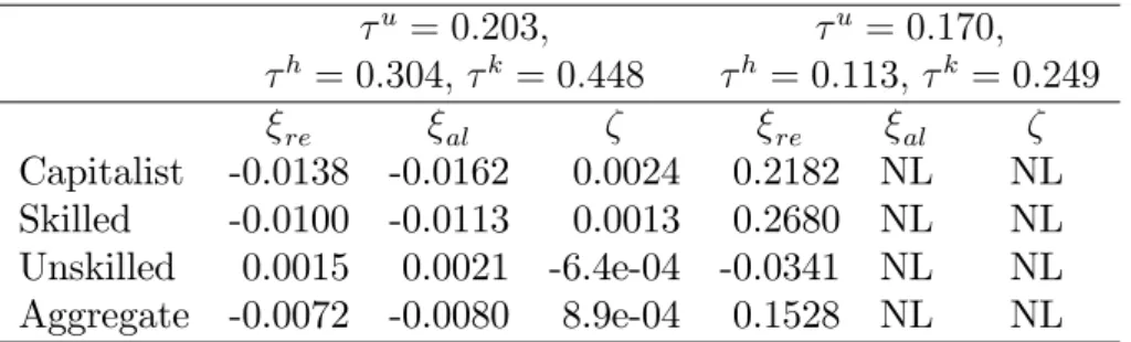
(1990), Cooley and Hansen (1992), Giannitsarou (2006) and Malley et al. (2009) by computing the percentage extra consumption that an individual would require so as to be equally well o¤ between the two regimes. This is de…ned as i;j i;j = Ui;jpost Ui;sspre ! 1 (1 ) 1 (39) for each agent i=c; s; u; aand each casej =re; al, wheressdenotes welfare calculated in the steady-state, re welfare under the rational expectations solution and al, welfare under adaptive heterogeneous learning. For all the cases below, in the case of homogeneous learning, the welfare e¤ects of tax reforms for all agents are e¤ectively the same as under the RE solution as in Giannitsarou (2006).38 Hence, to save on space, we do not discuss results
from this solution further. To quantify the importance of bounded rationality with heterogeneous initial beliefs for welfare, we also calculate the cost of the heterogeneous learning, compared to the rational expectations solution. This is de…ned as i;k i = Ui;repost Ui;alpost ! 1 (1 ) 1 (40) where i=c; s; u; a.
In Tables 3 - 6 below we report the welfare losses or gains for all agents under the di¤erent scenarios and policy regimes, calculated using the formu-las above. In Figures 1 - 4, we plot the tax revenue and debt La¤er curves, the pre-reform state in percent deviations from the post-reform steady-state and the transition paths of the four steady-state variables as well as con-sumption and labour hours for each agent, under rational expectations and learning. Each Figure corresponds to a particular tax reform case. The paths of consumption and hours are important as these will ultimately determine welfare for each agent.
5.3
La¤er curves in
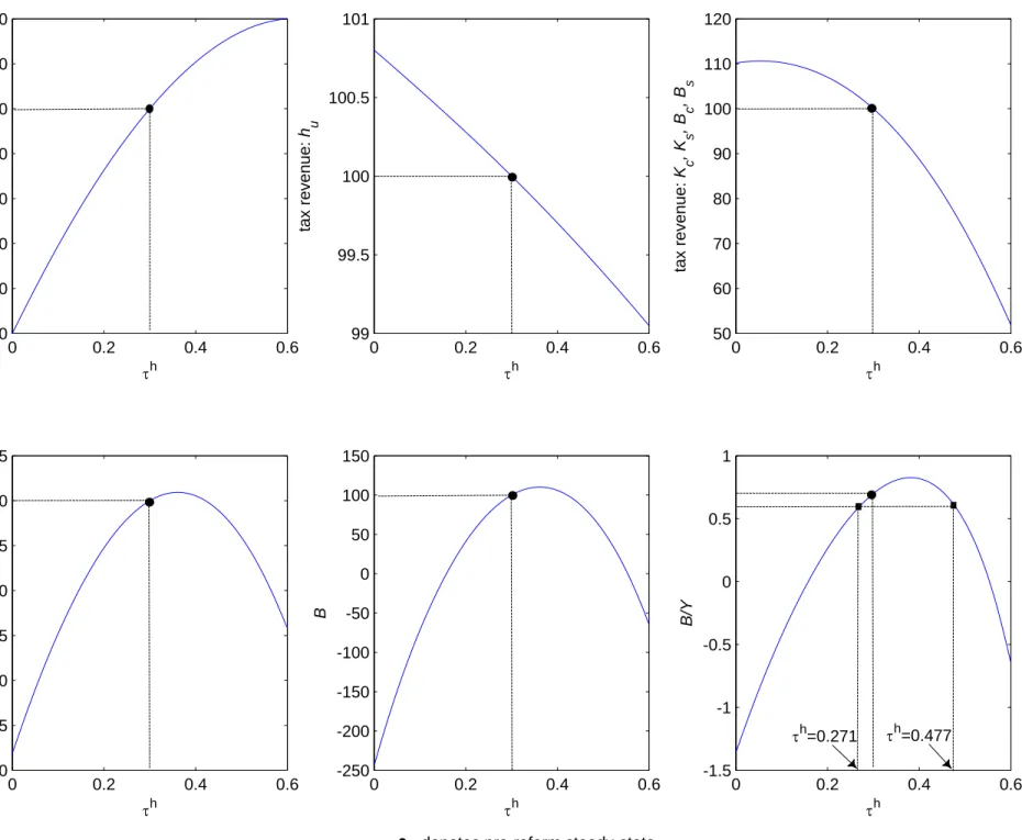
hThe La¤er curves associated with changes in hare shown in Figure 1a. These show the tax revenue collected and debt relative to the current steady-state, which is normalised to 100 for ease of presentation. For B=Y, we plot debt as a share of GDP. The pre-reform steady-state is also given on each La¤er
38Note it is only when the tax reform was accompanied by a positive or negative shock
to TFP that the rational expectations and learning transition paths more substantially di¤ered in Giannitsarou (2006).
curve in Figure 1a. We present those for a range of labour income tax rates that are consistent with a well-de…ned solution to the model.
As can be seen from the debt-to-GDP La¤er curve (lower right panel), the
B=Y target of 60% can be achieved by either increasing h to 47:7%, or by
decreasing it to27:1% from its pre-reform rate of30%. The required increase in h is large and essentially implies increasing the e¤ective average tax rate
for the upper70% of the income distribution to the e¤ective income tax that currently applies to highest income brackets (i.e. those with annual incomes above £ 200,000), when the National Insurance contributions are accounted for as well (see the average tax rates per income group in Social Trends 38, O¢ ce for National Statistics). This implies an increase in the progressivity of the e¤ective labour income tax system to 2:39, from less than 1:6 as it currently stands. In contrast, the required decreases in h are small, and
would result in decreasing the labour income progressivity ratio to 1:36. [Figure 1a about here]
The La¤er curve for labour income from skilled labour in Figure 1a (up-per left panel) indicates that the economy is always on the upward slopping part of this curve, at least for values of h that give a well-de…ned solution, so that increases (decreases) in h increase (decrease) tax revenue. The
pre-and post-reform steady-states for the increase in h are shown in Figure 1b.
As can be seen, the resulting fall in skilled labour supply causes a decrease in the supply of capital and unskilled labour, because of the complementari-ties in production. Given that the tax rates on capital and unskilled labour have not changed, the tax revenue collected from these two sources decreases, which is depicted in Figure 1a (upper right and upper middle panels respec-tively). These imply that the increases in total revenue when h increases are
smaller, as shown in the total revenue La¤er curve in Figure 1a (lower left panel), so that, for instance, an increase in h from 0:3 to 0:4 increases tax
revenue from skilled labour by about 20%, while leaving total tax revenue practically unchanged. Therefore, the complementarity between capital and labour implies that there is a La¤er curve between total tax revenue and h,
the peak of which is obtained for a value of h about 35% despite that fact
that we only obtained the upward slopping part of the skilled labour tax revenue La¤er curve.
[Figure 1b about here]
Of course, the e¤ects on tax revenue are reversed for decreases in h. As can be seen when comparing the pre- and post-reform steady-states for
falls in h in Figure 1c, when h (and thus also tax revenue from skilled
labour) decreases, there is an increase in skilled labour supply, which causes an increase in the supply of capital and unskilled labour, due to the comple-mentarities in production. Given that the tax rates on capital and unskilled labour have not changed, the tax revenue collected from these two sources increases so that the total tax revenue falls by less. For instance, when h
decreases from0:3to0:2, tax revenue from skilled labour falls by about40%, while total tax revenue falls by approximately 10%.
[Figure 1c about here]
It is interesting to note that although the complementarity between cap-ital and labour also exists in a standard Cobb-Douglas production function within a representative agent framework, the quantitative importance of the complementarities between the three di¤erent factor inputs is di¤erent in the heterogeneous agents setup, in light of the role of unskilled labour. Given that, as discussed in the calibration section, the elasticities of substitution between all three factor inputs considered here are well within those found in micro-econometric studies, the quantitative implications of these complemen-tarities is not without empirical foundation. As said above, it is essentially because of these complementarities that we obtain the La¤er curve in total tax revenue, which, in turn, implies that there will be a La¤er curve with respect to debt and thus two long-run solutions for reducing the debt by changing h.
5.3.1 Transition dynamics and welfare e¤ects
In Figure 1b we plot the dynamic transition from pre- to the post-reform steady-state for an increase in h and in Figure 1c for a fall in h. In Table
3 we calculate the welfare losses and gains for all agents in both cases. The …rst thing to note in Figure 1b is that the post-reform economy implies less consumption and less work time, for all agents, as a result of higher taxation. An increase in h hurts the capitalist and the skilled worker directly, but indirectly it also negatively a¤ects the unskilled worker. This happens because skilled labour complements unskilled, so that a decline in the former reduces the productivity of the latter. This trade-o¤ implies a fall in welfare for all agents in the post-reform economy, as can seen by the re measure in the …rst column of Table 3. Given that the e¤ects on the capitalist and the skilled worker are direct, they are hurt more by this change and hence
su¤er very big losses in welfare.
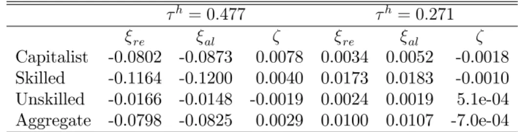
Table 3: Welfare costs/gains of reducing B=Y to0:6
h = 0:477 h = 0:271 re al re al Capitalist -0.0802 -0.0873 0.0078 0.0034 0.0052 -0.0018 Skilled -0.1164 -0.1200 0.0040 0.0173 0.0183 -0.0010 Unskilled -0.0166 -0.0148 -0.0019 0.0024 0.0019 5.1e-04 Aggregate -0.0798 -0.0825 0.0029 0.0100 0.0107 -7.0e-04 Adaptive learning increases the welfare costs, if we assume that capitalists and skilled workers form di¤erent initial beliefs about the economy and their policy functions. As can be seen in Figure 1b, the paths under heterogeneous learning deviate substantially and actually over- and under-shoot the rational expectations solution, as the agents learn and update their forecasts over time. In particular, the capitalist and the skilled worker overshoot in their decrease in consumption and undershoot the reduction in labour hours for long time periods. Both movements tend to reduce their welfare, compared to rational expectations. The additional losses, as reported in Table 3, are not trivial and amount to 0:78% of consumption for the capitalist and 0:4% for the skilled worker. The unskilled workers, forming no expectations, are not a¤ected as much by learning. They are actually better o¤ under learning, as their consumption is not reduced by as much, which more than compensates for the smaller increase in leisure time.
The results are reversed when h is decreased. As discussed above, the
increase in the labour supply of skilled labour crowds-in capital and unskilled labour, increasing the tax revenue collected and also consumption for all agents, as can be seen in Figure 1c. The trade-o¤ is now in favour of all agents, who are now better o¤ in the post-reform economy, as can be seen in Table 3. Hence, all agents in the economy would support a decrease in
h relative to the current steady-state. In addition, adaptive learning with
heterogeneous initial beliefs implies, in fact, small welfare bene…ts for the agents. Under heterogeneous learning, they overshoot their adjustment to the post-reform steady-state and hence they reap more quickly the bene…ts associated with the post-reform economy.
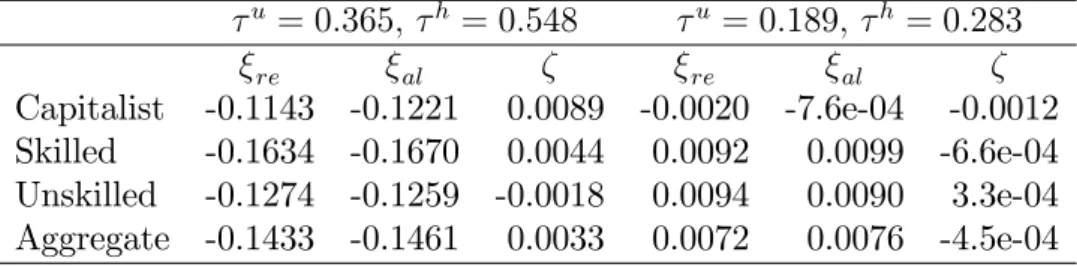
5.4
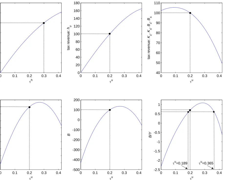
La¤er curves in
uand
hWhen both labour income tax rates are increased proportionately, they both need to increase signi…cantly, to 0:365 for u and 0:548 for h. On the contrary, small decreases, u = 0:189 and h = 0:283 would su¢ ce to reduce