Automating Workload Management for Enterprise-Scale Business Intelligence Systems: Old Problems Just Won t Go Away

Automating Workload Management for

Enterprise-Scale Business Intelligence Systems:

Old Problems

Just

Won’t Go Away

Umeshwar Dayal

[email protected]

Harumi Kuno, Janet Weiner, Kevin Wilkinson,

Abhay Mehta, Chetan Gupta

Intelligent Information Management Lab

Hewlett-Packard Labs

Palo Alto, CA, USA

Stefan Krompass , Alfons Kemper (TU Munich),

Archana Ganapathi (UC-Berkeley)

Outline

•

Context: Next Generation Business Intelligence

•

Workload Management Challenges

•

Predicting Query Performance

•

Managing Batch Workloads

•

Managing Interactive Workloads

•

Experimental Framework for Studying Mixed Workload

Business Intelligence Today

Technologies, tools, and practices for collecting, integrating, analyzing, and presenting large volumes of information to enable better decision making

• Strategic decision making: analytics by experts • Off-line, serial pipeline: batch ETL

(Extract-Transform-Load)

• Workloads run in isolation on different platforms

• BI is the #1 technology priority for CIO’s 2006-2008 • Market for BI is huge and growing (2006 numbers)

Business analytics market: $19B, 10.3% growth Data warehouse platform software market: $5.7B, 12.5% growth

BI services market (data integration, DW design, and vertical solutions): $31B

Analysis Operational System Operational System Operational System Reporting Applications ETL

Next-Generation BI: Operational BI

•

Bringing BI into the “mainstream”

Operational System High Ingest

Analysis

Systems, Sensors, External feeds, Structured & Unstructured info, with

near-real time extraction and integration

Model Building Models Operational System RT Model Execution Operational System Data Access Analytic Applications •

A change in concurrency,

reliability, workload profile

•

Yesterday: Small

number of back office

power users

•

Tomorrow: 10,000

users perform

business actions…

dozens of times a day

•

Near real-time: no end-to-end

latency

•

Mixed workloads

•

Robust, predictable

performance

•

Integrate structured &

less-structured data

•

Gartner: 90% of Global

2000 will have

mission-critical DW applications in

place in the next 5 years

Operational BI: Research Challenges

Extraction & Integration

Analytics

Online Analytic Applications

OLTP External Feeds Streams/Events

Operational data store

Online Operational Systems

Transactional Storage Manager Relational Query Processor

Parallel Data Warehouse

Operational BI Platform

Delivery and Interaction

Self-managing: automated design, tuning, and

maintenance

Highly parallel computer architectures, multi-core

processors, storage hierarchies “Low latency” data integration pipeline

End-to-end optimization

Integration of structured and less structured data

Visual interaction and collaboration interfaces

Robust, stable performance Highly scalable & available

Mixed Workloads Continuous, on-line updates Complex batch and ad hoc

queries

Massively scalable analytics

Outline

•

Context: Next Generation Business Intelligence

•

Workload Management Challenges

•

Predicting Query Performance

•

Managing Batch Workloads

•

Managing Interactive Workloads

•

Experimental Framework for Studying Mixed Workload

Mixed Workload Performance Management

•

Enterprise Data Warehouses are very

complex and expensive to manage.

•

Hundreds of ‘knobs’

•

Workloads are becoming

increasingly complex and dynamic

(especially for operational BI)

•

Some queries run in seconds,

some take hours

•

Mixed workloads

•

Batch (rollups, reports), interactive

(ad hoc queries)

•

Different performance objectives

•

Some are urgent, some have

lower priority

•

Automation is needed

"An Enterprise Data Warehouse must service a wide spectrum of queries: from simple, sub-second lookups, to complex multi-hour rollups. An EDW is expected to

provide the best response time for on-demand queries while simultaneously meeting deadlines for batch queries. All of this must be done without overloading (or under-loading) the system, and with effective controls for rogue queries. This is a difficult problem. Managing the query workload effectively is one of the major challenges in running an EDW.“

Managing data warehouse performance is like

juggling feathers, golf balls, bowling balls, …

Through 2010, mixed workload performance will remain the single most important performance issue in data warehousing [Gartner].

Workload Management Problems

•

How long should this query take?

•

With other queries running concurrently?

•

What resources will it consume?

•

Should we allow this query into the system?

•

When should we start the query?

•

Will this query ever finish? When?

•

What should we do if it is taking too long?

•

Wait?

•

Kill it?

•

Kill it and restart it? When?

•

Kill some other query? Which one?

performance

prediction

progress

indicator

execution

control

admission control

workload

scheduling

Workload Management Approach

•

Machine learning models for predicting performance of queries and

workloads

•

Predict query run times under load

•

Simultaneously predict multiple performance metrics:

cpu time, memory usage, message bytes, disk I/O, ...

•

Experimental Framework

•

Create a taxonomy of problem queries and operational BI

workloads

•

Simulate system configurations, workload execution & workload

management policies

•

Systematically study the ability of workload management policies to

deal with problem workloads

4. Early Warning System

Load

2. Query Workload Management

SLAs SLOs E X E C U T I O N E N G I N E S L A M A N A G E R Workload Scheduler Q U E R I E S Query Queue 1 Queue 2 Queue k Execution Manager

1. Prediction of Query Runtime

Query Optimizer

Workload + Query Optimizer Cost Estimates

Workload +Dynamic Query Cost Estimates

System Load

Execution Cost

Control

Workload

System Load and Execution Cost

3. Query Progress Indicator

Admission Control

Workload Management Architecture

Statement Name:Query_101 18%

Query Progress Indicator Elapsed Time:53.22

Current Time (t*):25th August 2006 16:24:40 Estimated Cost:352 dop Query Execution Speed (at t*):1.2 dop/min Estimated Query Time Left:4:09:20

Outline

•

Context: Next Generation Business Intelligence

•

Workload Management Challenges

•

Predicting Query Performance

•

Managing Batch Workloads

•

Managing Interactive Workloads

•

Experimental Framework for Studying Mixed Workload

Currently, no good way to estimate

execution time*

Cost as a predictor of Execution time

(559 HPIT Canned reports and Yotta generated queries)

y = 0.2206x + 13.067 R2_{= 0.0766} 0 10 20 30 40 50 60 70 80 90 100 0 5 10 15 20 25 30 Cost Time Taken

RMS Error = 26.70

Prediction of Query Run Time (PQR)

•

Predict the execution time of a query,

allowing the user to trade off accuracy

and precision.

• Learn from execution histories

• Understand the problem as that of

classification with unknown classes.

• At the heart of this approach is a machine

learning model called PQR Tree (Prediction

Of Query Runtime).

• Approach:

• From historic data extract features that describe the query plan and the system load.

• Train a PQR Tree on these features.

• For a new query extract its plan and load

features.

• Apply the PQR Tree on these features to

predict the time range of the new query.

A. Mehta, C. Gupta, U. Dayal, “PQR: Predicting Query

Execution Times for Autonomous Workload Management” Proc. Intl Conf on Autonomic Computing, 2008.

Historic Queries Extract Features Plan & Load Vectors P1, P2: Construct Tree PQR Tree New Query Extract Features Plan & Load Vectors P3: Apply Tree [Predicted execution time range] Obtaining a PQR Tree Obtaining a time range for a new query Historic Queries Extract Features Plan & Load Vectors P1, P2: Construct Tree PQR Tree New Query Extract Features Plan & Load Vectors P3: Apply Tree [Predicted execution time range] Obtaining a PQR Tree Obtaining a time range for a new query Historic Queries Extract Features Plan & Load Vectors P1, P2: Construct Tree PQR Tree PQR Tree New Query Extract Features Plan & Load Vectors P3: Apply Tree [Predicted execution time range] Obtaining a PQR Tree Obtaining a time range for a new query

PQR Tree

• A PQR Tree, denoted by T_s, is a binary

tree such that:

1. For every node u of T_s, there is an associated 2-class classifier f_u.

2. The node u contains examples E_u, on which the classifier f_u is trained.

3. f_u is a classifier that decides for

each new query q with execution

time t_q in [t_ua , t_ub], if q should go to

[t_ua,t_ua+•) or [t_ua+•, t_ub], where •

lies in (0, t_ub-t_ua).

4. For every node u of T_s, there is an

associated accuracy, where

accuracy is measured as the percentage of correct predictions made by f_u on the example set E_u.

5. Every node and leaf of the tree

corresponds to a time range.

N1: fu= Classification Tree, [1 – 2690] 93.5% N11: fu= Classification Tree [1 – 170) N12: fu= Classification Tree [170 – 2690) 100% _84.6% 87.5% N111:= [1 – 13) N112 [13 – 170) N121 [170 – 1000) N122:fu= Tree [1000 – 2690) N1221 [1000 – 1629) N1222 [1629 – 2690)

Feature Vectors

•

Query Plan Vector

• Select features through enumeration,

construction and domain expertise.

• Bushiness, Disk Partition Parallelism, Process

Parallelism, Number of IOs, IO Cardinality, IO Cost, Non-IO Cost, Number of Joins, Join Cardinality, Number of Probes, Table Count, Number of Sorts, Sort Cardinality, Total Cost, Total Estimated Cardinality, etc.

•

Load Vector

• The CPU characteristics tend to be erratic and

unpredictable.

• ``Stretch’’ of a query is a good indicator of the load the query experiences while running.

• MPL is a determining factor for stretch and a

good variable for prediction. Hence the new load vectors:

• Query Stretched Cost, Query Stretched Process Parallelism, Query Stretched Operator Cost, Process stretched cost, Process stretched Process parallelism, Process stretched Operator Cost

SELECT n.name

FROM tbNation n, tbRegion r WHERE n.region = r.region

AND r.name = 'EUROPE' ORDER BY n.name; root exchange sort split split partitioning partitioning file_scan file_scan [ tbNation ] [ tbRegion ] nested_join

Creating the PQR Tree

•

Recursively create nodes till one of the

termination conditions

is met:

•

Time range is too small.

•

Number of training examples is too small in a node.

•

Accuracy of prediction falls below a threshold.

•

To

create

a node:

•

Take all the queries in the training set and arrange them in ascending order

of running time. Each running time is a potential point at which the time

range for the node can be split.

•

For every classifier in a fixed set of classifiers compute accuracy for each

potential split point.

•

Chose the combination of classifier and the split that has the highest

accuracy on the test set.

•

Enhancements:

•

Top K

: Compute the percentage change between successive values in this

list. Chose some fixed number of largest changes. They are potential split

points.

•

Skip Split Points

: Skip

n

_skip

percent points from both ends of an interval as

Applying PQR Tree

•

Predict

the time interval for the execution time of a new query.

•

Decompose the query and the system load into the feature vector

described earlier.

•

Apply the classifier at each node to this feature vector, to determine

whether this new query belongs to the left or the right child.

•

Do this recursively at each node until we reach a leaf of the PQR

tree.

•

The leaf has a time range associated with it and this becomes the

predicted execution time of the new query.

•

As the range of execution times becomes narrower corresponding to a

greater depth in the tree, the prediction accuracy will be lower. This

approach allows the user to choose a time range they are comfortable

with.

Resulting Prediction of Query Runtime

(PQR) Model – Loaded system

N1: F = Classification Tree, [1 – 2690] 93.5% N11: F = Classification Tree [1 – 170) N12: F = Classification Tree [170 – 2690) 100% _84.6% 87.5% N111: Tree [1 – 13) N112: Tree [13 – 170) N121: Tree [170 – 1000) _{[1000 – 2690)}N122: Tree N1221 [1000 – 1629) N1222 [1629 – 2690) 37.1% Total Opera tor Cost 55.9% Static PQR 86.5% 36.5% Accura cy Prediction of Query Runtime (PQR) Optimi zer Cost

PQR Results – TPC-H

MPL = 10 MPL= 8 MPL = 6 MPL = 4

Accuracy Buckets Accuracy Buckets Accuracy Buckets Accuracy Buckets Test 1 85.585586 6 89.344262 6 88.571429 5 91.176471 6 2 80 9 73.831776 9 83.157895 11 88.888889 9 3 84 5 84.210526 6 85.714286 8 87.610619 8 4 85.185185 9 87.5 3 80.869565 10 88.461538 10 5 75.490196 11 88.043478 8 82.653061 9 79.381443 8 6 88.77551 7 84.090909 10 87.5 7 91.304348 9 7 81.632653 6 92.66055 9 80.412371 10 84.782609 8 8 75.247525 6 67.567568 8 85.542169 10 90.425532 7 9 85.454545 8 81.132075 9 91.891892 5 89.07563 6 10 75.229358 8 87.628866 7 81.521739 5 82.978723 6 Avg 81.6600558 7.5 83.601001 7.5 84.7834407 8 87.4085802 7.7

Results on a real customer workload

Accuracy vs Time Ranges for Customer X Database (Workload # 2)

0 2 4 6 8 10 12 0 10 20 30 40 50 60 70 80 90 100 Accuracy

Number of Time Ranges

Accuracy vs Time Ranges for Customer X Database (Workload # 3)

0 2 4 6 8 10 12 14 16 18 0 10 20 30 40 50 60 70 80 90 100 Accuracy

Number of Time Ranges

Accuracy vs Time Ranges for Customer X Database (Workload # 2)

0 2 4 6 8 10 12 0 10 20 30 40 50 60 70 80 90 100 Accuracy

Number of Time Ranges

Accuracy vs Time Ranges for Customer X Database (Workload # 3)

0 2 4 6 8 10 12 14 16 18 0 10 20 30 40 50 60 70 80 90 100 Accuracy

Number of Time Ranges

Beyond Run-time Prediction: Predicting

Multiple Performance Metrics

•

Goal:

•

For a specific machine configuration …

•

Predict performance of a query run at MPL=1

•

Using only the query and compiler output

•

Predict execution time, cpu time, message bytes, disk i/o,…

•

Predict performance of a workload run at given MPL > 1

•

Applications:

•

Initial sizing

•

What system configuration for a given workload?

•

Capacity planning

•

What happens to performance when workload or configuration

changes?

•

Workload management

•

What to expect from queries, workload?

SELECT n.name

FROM tbNation n, tbRegion r

WHERE n.region = r.region

AND r.name = 'EUROPE'

ORDER BY n.name;

root

exchange

sort

split

split

partitioning

partitioning

file_scan

file_scan

[ tbNation ]

[ tbRegion ]

nested_join

4.5 2 2 5 1 5 1 4.5 2 2 5.00 1 7.02 2 5.00 1 split sort root partitioning nested_join file_scan exchange 4.5 2 2 5 1 5 1 4.5 2 2 5.00 1 7.02 2 5.00 1 split sort root partitioning nested_join file_scan exchange N u m ber of instances of the operator in query Sum of cardinalities for each instance of the operator

Create Query Vector from Compile-Time

features for input to prediction

Query Plan Projection

Performance Projection 0 LP PL 0 LL 0 0 PP A B = A B

Matrices showing

similarity of query

pairs using a

Gaussian kernel

function

2E4 23E5 80E2 1.4E4 Op2 Op1 Query Plan Query Plan Feature Matrix Statistics Elapsed Time Execution Time I/Os …

Training (through Kernel Canonical

Correlation Analysis - KCCA)

Compile-time features

Run-time features

Performance Feature Matrix 7.3E3 23839 27E2 4.3E7 … I/O Time 1 … N 1 : N Query Plan Similarity Matrix 1 … N 1 : N Performance Similarity Matrix

Co-locate

queries based

on plan AND

performance

features

L

P

L X A

P X B

KCCA

Query Plan

Projection

Performance

Projection

Query Plan

3E 80E 1.4E

Compile-time Feature

Vector

nearest

neighbors

Predicted

Performance

Vector

8E 25792 128

0.01 0.1 1 10 100 0.01 0.1 1 10 100

KCCA predicted elapsed time

actual elapsed time

Under-estimated

records accessed

disk i/o

estimate

too high

1 hour

1 second

1 minute

1 second

_{1 minute}

1 hour

Perfect

prediction

Results: Predicted vs. Actual Elapsed Time

Actual elapsed time

0.0001 0.01 1 100 10000 0.0001 0.01 1 100 10000 Optimizer Cost

Actual Elapsed Time

Cost estimate

10x away from

best fit

Line of best fit

Cost estimate

100x away from

best fit

Optimizer Cost Estimates

Optimizer Cost Estimates

Actual Elapsed Time

1 hour

1 second

1 minute

Cost estimate

100x away from

best fit

1.00E+00 1.00E+01 1.00E+02 1.00E+03 1.00E+04 1.00E+05 1.00E+06 1.00E+07 1.00E+08 1.00E+0 0 1.00 E+01 1.00E+021.00E+0 3 1.00E+0 4

1.00E+051.00E+061.00E+0

7

1.00E+0

8

KCCA predicted records used

actual records used

Perfect prediction Under-estimated

records accessed

Performance Prediction Summary

•

Predict performance for queries AND workloads

• Train and predict for a given configuration (hardware / software / MPL)

• Predict using only query plan features of new queries.

•

Test results show good prediction accuracy

• Predict multiple aspects of performance: cpu time, memory usage, message bytes,

disk I/O, ...

• Multiple metrics useful: explain inaccuracies; Suggest which queries to run together

(complementary use of memory, disk) •

Training is time-consuming

• Many hours to run queries and workloads; Few hours to train models

•

But prediction is fast: only 10-15 seconds per query

•

Continuous retraining will be needed

A. Ganapathi, H. Kuno, U. Dayal, J.Wiener, A. Fox, M. Jordan. D. Patterson, “Predicting Multiple Metrics for Queries: Better Decisions Enabled by Machine Learning.” Proc. ICDE 2009.

Outline

•

Context: Next Generation Business Intelligence

•

Workload Management Challenges

•

Predicting Query Performance

•

Managing Batch Workloads

•

Managing Interactive Workloads

•

Experimental Framework for Studying Mixed Workload

Batch Workload Management

•

Maximize the throughput of BI batch

workloads (while protecting against

underload and overload)

•

Intuition

:

•

Find a good ‘

manipulated variable

’.

•

Make the system stable over a wide

range of this ‘manipulated variable’.

•

Target somewhere in the middle of

the range

•

MPL

has been used but:

•

The optimal mpl is a lower number

for resource-intensive queries,

whereas the optimal mpl is higher

for less intensive queries.

•

A typical BI workload can fluctuate

rapidly between long, resource

intensive queries and short, less

*MPL = Number of concurrent streams

MPL

Throughput

Under-load Overload (thrashing) Optimal range LARGE WORKLOAD MEDIUM WORKLOAD Target

Peak Memory Consumption – A Better

Manipulated Variable

SF100

SF400

SF200

Abhay Mehta, Chetan Gupta and Umeshwar Dayal, BI batch manager: A system for managing batch workloads on enterprise data-warehouses. EDBT 2008: 640-651, Nantes, France.

PGM (Priority Gradient Multiprogramming)

•

‘m’ concurrent streams (MPL=m)

•

Each running at an equal priority (eg

148)

•

‘m’ concurrent streams (MPL = m)

•

Each running at a DIFFERENT priority

(eg 148, 146, 144, 142,…, 148-2(m-1))

…

…

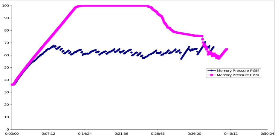
Priority Gradient Multiprogramming

PGM

Equal Priority Multiprogramming

33 0 10 20 30 40 50 60 70 80 90 100 0:00:00 0:07:12 0:14:24 0:21:36 0:28:48 0:36:00 0:43:12 0:50:24 Memory Pressure PGM Memory Pressure EPM

Figure : Memory Pressure Curves for EPM and PGM Schemes

PGM Protects Against Overload…..

•

PGM is stable and exhibits saw-tooth pattern of acquisition, consumption and

release.

•

EPM shows the concurrent buildup of memory resulting in overflow.

…. Hence, stabilizes execution across

memory prediction errors

1F

1/kF

kF

PGM PGM PGM EPM EPM EPM SF100 SF200 SF400

Reasons for stability:

- PGM is unfair

- Quick release

Complex Workload - Q4 0 20 40 60 80 100 120 140 0 2 4 6 8 10 12 14 16 Memory Throughput MPL SF 100 MPL SF 200 MPL SF 400

Outline

•

Context: Next Generation Business Intelligence

•

Workload Management Challenges

•

Predicting Query Performance

•

Managing Batch Workloads

•

Managing Interactive Workloads

•

Experimental Framework for Studying Mixed Workload

Interactive Workloads: Scheduling

49 51 ART = 74.50 AS = 1.48 51 49 ART = 75.50 AS = 1.52 1 99 ART = 50.50 AS = 1.00 ART = 99.50 AS = 50.50 1 99

OLTP

BI

a)

b)

c)

d)

49 51 ART = 74.50 AS = 1.48 49 51 ART = 74.50 AS = 1.48 51 49 ART = 75.50 AS = 1.52 51 49 ART = 75.50 AS = 1.52 1 99 ART = 50.50 AS = 1.00 1 99 ART = 50.50 AS = 1.00 ART = 99.50 AS = 50.50 1 99 ART = 99.50 AS = 50.50 1 99

OLTP

BI

a)

b)

c)

d)

0 5000 10000 15000 20000 25000 30000 0.1 1 10 100 1000 10000

Query Size (Seconds)

Frequency

Stretch = (p

_i

+ w

_i

)/p

_i

Design a strategy for the online scheduling of queries on

an Enterprise Data Warehouse.

Criteria for a ‘good’ Online Scheduler

FEED

•

F

air

•

Avoid starvation of queries

•

Lower the ‘max’, or the ‘variance’ of query times

•

E

ffective

•

The majority of queries should do well

•

Lower the ‘average’

•

E

fficient

•

The strategy should be lightweight

•

Computational complexity of implementation should be sub-linear

•

D

ifferentiated

•

Different service levels should give differentiated performance

without unduly penalizing the overall avg and max.

How our scheduler works

•

Maintain a queue of queries ordered by their ‘rank’.

•

When a new query is submitted, compute its ‘rank’, and

insert it into the queue in the order of its ‘rank’.

•

Run the queries in the order of their ‘rank’, with ‘Highest

Rank First’

DBMS

DBMS

rank?

Ordered by

decreasing ‘rank’

_{How is rank computed?...}

Design the ‘rank’ function using the

FEED criteria

1.

Start with a proven ‘effective’ algorithm (SJF) :

r = 1/p

, w

here ‘

p

’ is the estimated cost of the query

2.

Add a wait component that achieves ‘fairness’:

r = 1/p + Kw

,

where

K

is a constant, and

w

is the wait

time of the query

3.

Include a component that allows differentiation between

service levels:

r = •/p + Kw

,

where

•

indicates the service level

4.

Implementing this function as a queue has a sub-linear

computational complexity

Computing the Parameters

•

Based on the value K, rank function (

r = •/p + Kw

) generalizes known

scheduling functions:

•

SJF: K=0

•

FIFO: K > 1 -1/• where

• is the execution time of the longest query

•

Tradeoff between fairness and effectiveness

•

0 < K < 1 -1/•

•

Derive a value for K

•

With this value, provably does not cause starvation

•

Mapping Service Levels: The ratio

r

of stretches of a query of size p

with service level • and 1 can be computed as:

•

For Pareto Distribution:

1, , , , / p p p p

T

T

p

r

T

T

p

∆ ∆ ∆ ∆

+

+

=

+

+

1 (r 1)(N ln p N ln p p) N N ∆ ∆ − + + +

∆ =

2

1

K

ψ

=

Experimental Setup

•

Model workloads

•

Pareto Distributions

•

Optimizer Cost Estimate

•

Actual Processing Time

•

Study L

₂

norm for Stretch

•

Study differentiation: Two models for

rFEED

:

rFEED

₁

&

rFEED

₁₀

•

Compare with an optimal resource slicing system

RS

_OPT

•

Study Peak Load and Steady State Load

L ₂ = (p₁2 _{+ p}

Execution Time With Pareto Distribution

(Steady State)

L2Norm for Pareto Distribution with Steady State Load

0 0.5 1 1.5 2 2.5 3 3.5

Overall Highest SL Medium SL Lowest SL

Metric

Ratio

RSopt rFeed1 rFeed10

Execution Time with Optimizer Estimate

(Peak Load)

L2Norm for Cost with Peak Load

0 5 10 15 20 25 30 35 40

Overall Highest SL Medium SL Lowest SL

Metric

Ratio

RSopt rFeed1 rFeed10

Outline

•

Context: Next Generation Business Intelligence

•

Workload Management Challenges

•

Predicting Query Performance

•

Managing Batch Workloads

•

Managing Interactive Workloads

•

Experimental Framework for Studying Mixed Workload

Experimental Framework for Workload

Management

•

It’s non-trivial to gauge the

impact of system configuration

and workload on a BI system’s

performance . . .

Gives you knobs to control:

• Workload characteristics: problem queries,

variance

• Workload Management policies: admission

control, scheduling, execution controls

• Multi-programming levels

• Resource models and behavior

So you can see:

• Impact of admission control, scheduling,

and execution control policies policies

• Impact of problem queries

• Impact on different objectives (e.g.,

complete 100% workload, minimize makespan, maximize useful work

Workload Management Actions

Execution Control Actions

Workload Management Policies

Execution Controller

Database Execution control Fuzzy Controller 0,5 0,75 0,25 0 1 0, 5 0,75 0,25 1 Current State Query n Query 1 ... data actions

Runtime statistics & Query information

Execution engine

IF relExecTime IS high AND (Progress IS low OR

Progress IS medium)

THEN cancel IS applicable

IF relExecTime IS high AND (Progress IS high

Preliminary Results from Experimental

Framework

•

Huge variance in query sizes and resource demands

•

Short queries: wait time can outweigh execution time

•

Long queries: even a few can significantly slow system

•

Admission control is effective when execution cost estimates ore accurate

•

When execution costs are underestimated, threshold-based execution

control actions have to be taken

•

But need guidelines for setting thresholds

•

Corrective actions against long-running queries can help, but

•

Overly aggressive actions can hurt performance

•

Simple actions (kill, resubmit) about as effective as newly proposed

actions (suspend/resume)

S. Krompass, H. Kuno, U. Dayal, A. Kemper, “Juggling Feathers and Bowling Balls” VLDB 2007. S. Krompass, H.Kuno. J.Wiener, U. Dayal, K.Wilkinson, A Kemper, “Managing Long Running Queries.” HPL Tech Report, 2008.

Example of Experimental Results

Impact of problem queries

_{Impact of control actions}

Interactive jobs