Numerical Simulations of Transition due to Isolated
Roughness Elements at Mach 6
Jeroen P. J. P. Van den Eynde∗and Neil D. Sandham†
University of Southampton, Southampton, England SO17 1BJ, United Kingdom DOI: 10.2514/1.J054139
An accurate prediction of transition onset behind an isolated roughness element has not yet been established. This is particularly important in hypersonic flow, where transition is accompanied by increased surface heating. In the present contribution, a number of direct numerical simulations have been performed of a Mach 6 boundary layer over a flat plate with isolated roughness elements. The effects of roughness shape, planform, ramps, and freestream disturbance levels on instability growth and transition onset are investigated. It is found that the frontal shape has a large effect on the transition onset, which is in agreement with previous studies, whereas the roughness element planform has a marginal influence. A new result is that the roughness shape in the streamwise direction (in particular, the aft section) is also an important characteristic, since an element with a ramped-down aft section allows the detached shear layer to spread out and weaken, leading to a lower instability growth rate. Above a critical value, the instability growth rate is found to be correlated with the amplitude of the low-speed streak formed by the roughness element, suggesting that a more physically based transition criterion should take account of the local liftup effect of the particular roughness shape.
Nomenclature Ast = streak amplitude
a = disturbance amplitude
by = stretching factor
Cp = specific heat at constant pressure Cv = specific heat at constant volume cf = skin-friction coefficient c1;2;3;4 = constants D = roughness diameter E = total energy e = disturbance energy F = nondimensional frequency
Ie = integrated disturbance energy
k = roughness height
L = length
Lsep = separation length
M = Mach number
N = number of grid points
Pr = Prandtl number
p = pressure
Q = second invariant; momentum deficit
q = heat flux vector
R = universal gas constant
Re = Reynolds number
Syz = roughness projected frontal area S = Sutherland’s temperature
T = temperature
t = time
U∞ = freestream velocity
u,v,w = streamwise, wall-normal, and spanwise velocities
us = shear magnitude
W = roughness width
w = local roughness width
β = spanwise wave number
γ = ratio of specific heats
δij = Kronecker delta function
δ0 = displacement-layer thickness
δ99 = boundary-layer thickness
λ = thermal conductivity
μ = dynamic viscosity
ρ = density
τij = viscous stress tensor
ϕ = phase
ω = circular frequency
Subscripts
r = reference value
x,y,z = streamwise, wall-normal, and spanwise components
Superscripts
^ = coordinate relative to plate leading edge
= dimensional variable
~ = coordinate relative to roughness center
0 = fluctuation with respect to base flow
I. Introduction
T
RANSITION from laminar to turbulent flow has been an active field of research for several decades. The various mechanisms that can lead to boundary-layer transition in incompressible flows are reasonably well understood, owing to the large number of experiments and numerical analyses performed since the 1950s. The traditional “natural” path to transition involves small-amplitude primary unstable disturbances entering the boundary layer through a receptivity process and following a linear instability process until they reach a sufficiently high amplitude to provoke secondary instabilities, which generate structures that subsequently break down into turbulence. When the freestream environment is noisier (i.e., an environment that contains disturbances that have a high enough amplitude to bypass this traditional path), different mechanisms will be responsible for the transition to turbulence. The presence of surface curvature and surface roughness, either distributed or isolated, can also have a great influence on the transition process. An extensive review of the different paths to transition in incompressible flow is given by Reshotko [1].Roughness-induced transition is of crucial importance in the design of hypersonic vehicles, since surface roughness generally
Presented as Paper 2014-2499 at the 7th AIAA Theoretical Fluid Mechanics Conference, Atlanta, GA, 16–20 June 2014; received 18 December 2014; revision received 23 March 2015; accepted for publication 24 April 2015; published online 23 July 2015. Copyright © 2015 by J. P. J. P. Van den Eynde and N. D. Sandham. Published by the American Institute of Aeronautics and Astronautics, Inc., with permission. Copies of this paper may be made for personal or internal use, on condition that the copier pay the $10.00 per-copy fee to the Copyright Clearance Center, Inc., 222 Rosewood Drive, Danvers, MA 01923; include the code 1533-385X/15 and $10.00 in correspondence with the CCC.
*Ph.D. Candidate, Faculty of Engineering and the Environment; j [email protected].
†Professor, Faculty of Engineering and the Environment; n.sandham@ soton.ac.uk. Senior Member AIAA.
Article in Advance / 1
promotes early transition; and the resulting increased skin friction and aerothermal heating might be catastrophic if transition is incorrectly predicted. For example, transition on the space shuttle orbiter during reentry occurred usually up to a Mach number of eight [2], but protruding gap fillers were found to act as discrete surface roughness and promote transition at higher Mach numbers [3], which might bring the aerothermal surface heating of the vehicle outside its allowable envelope. Even though roughness-induced transition in high-speed flows is of such importance, the mechanisms responsible for it are only partially understood and prediction of transition still relies mainly on engineering correlations from flight-test data and wind-tunnel experiments. These correlations have limited applicability outside the range (vehicle geometry, flight conditions, etc.) for which they were developed and do not give an insight into the physical processes of roughness-induced transition. Transition to turbulence is highly affected by the level and type of freestream disturbances, which has made it difficult to give accurate predictions of in-flight transition (where the disturbance environment is relatively quiet) by means of experiments in generally noisy wind tunnels. Only quiet wind tunnels [4], designed specifically for high-speed transition experiments, provide useful transition data to cor-relate with flight-test results; and experiments can be performed that give a better understanding of the physical mechanisms of roughness-induced transition. However, quiet wind tunnels are also limited, since they cannot match full-scale flight conditions of the Reynolds number, Mach number, and enthalpy. Therefore, it is currently impossible to reproduce full hypersonic flight conditions in a single ground-test facility. Direct numerical simulations (DNSs) can also be used to study the roughness-induced transition process and make it possible to obtain data and measurements that would not be possible using wind-tunnel experiments. Due to the high computational cost, however, DNSs of high-speed roughness-induced transition have only been performed recently, e.g., Marxen and Iaccarino [5], Choudhari et al. [6], Redford et al. [7], Groskopf et al. [8], Bernardini et al. [9], and De Tullio and Sandham [10], among others. DNS has its own set of limitations (e.g., the potential dependency on grid quality and numerical dissipation, and the need to prescribe an external forcing or noise source). Due to the high computational cost, the Reynolds numbers commonly obtained in flight cannot yet be simulated using DNS.
Surface roughness can be classified as isolated or distributed. Early attempts to confirm a Tollmien–Schlichting (T-S) mechanism, known to be of importance for transition behind two-dimensional surface roughness, for the transition due to three-dimensional distributed roughness proved fruitless [11]. A process distinct from the two-dimensional T-S instability mechanism is needed to explain the rapid growth of disturbances observed even in regimes tra-ditionally considered subcritical. Reshotko and Tumin [12] used wind-tunnel and ballistic test data for hypersonic zero-pressure gradient and stagnation flows combined with computations of the linearized Navier–Stokes equations and presented a model for transition due to distributed roughness that uses transient growth as the governing mechanism. They proposed that transient growth might be an explanation for early transition observed over distributed roughness elements.
Groskopf et al. [13] performed DNS and spatial biglobal analysis of Mach 4.8 flow over a three-dimensional isolated roughness element and found that, although absolute instabilities could occur at the recirculation zones around the roughness element, it is the trailing vortices and streaks generated behind the isolated roughness element that lead to strong convective instabilities in the shear layer above the streaks. The shear layers in the wake of the roughness can sustain two types of instabilities: sinuous (sometimes called odd or anti-symmetric), associated with the detached wall-normal shear layer; and varicose (or even/symmetric) modes concentrated near the regions of high spanwise shear at the sides. Varicose modes are usually more unstable [14,15] than sinuous modes, but it is not completely understood how they depend on the roughness geometry and flow conditions. Choudhari et al. [6] found that, for lower roughness height, the sinuous modes were dominant, whereas the varicose modes became dominant for a roughness element with larger
height. Wall cooling at Mach 3 and 6 was found to have a stabilizing influence [7,9], which was explained in work by De Tullio and Sandham [10] as a stabilization of the wake modes. The experimental measurement of roughness wake instability at hypersonic speed is difficult, due to the high structural loads on measurement probes, and not many studies have been published that cross validate experi-mental and numerical results of hypersonic wake instability. The first experimental detection of hypersonic wake instability was presented by Wheaton and Schneider [16], who studied the Mach 6 flow behind a cylindrical roughness element and found the instability to be largest away from the roughness centerline. Subbareddy et al. [17] performed DNS approximately matching the experimental con-ditions of Wheaton and Schneider [16], and they confirmed some of the experimental findings.
To predict whether or not roughness will cause transition, engineering correlations based on wind-tunnel experiments and flight-test data are still used. A good review and historical overview of the transition correlations commonly used are given by Reda [18]. Traditionally, a critical Reynolds numberRekk(sometimes denoted
byRek), based on roughness heightkand flow parameters at heightk
in the undisturbed flow, has been used as a transition criterion. Originally developed for incompressible roughness-induced tran-sition, the performance ofRekkas a transition criterion diminishes for
high-speed flow; and laminar cases have been reported with a Reynolds numberRekkwell above the critical values often quoted in
literature [9]. Redford et al. [7] investigated compressibility effects on roughness-induced transition at Mach 3 and Mach 6 and found they could separate the subcritical and transitional cases using a critical Reynolds numberRekkdependent on the Mach number in the
surrounding boundary layer at the roughness heightMk and wall
temperatureTw. They proposed a map ofMkT∞∕TwagainstRekk, for
which the dividing line between laminar and transitional simulations was given by
MkT∞∕Tw3Rekk−300∕700 (1)
Bernardini et al. [9] modified Redford et al.’s [7] transition map and used a modified transition Reynolds numberRekw(sometimes
denoted byRek), for which the reference viscosity was taken at the wall instead of at the roughness height. In the modified transition map, the critical line would be independent ofMkT∞∕Tw, and thus a
constant value. The inherent flaw of these roughness criteria is that they do not take into account the roughness geometry or freestream disturbance environment in any way. In an effort to overcome the former drawback, a roughness Reynolds number based on momentum deficit was presented by Bernardini et al. [19], which included the roughness frontal shape and aspect ratio. If a mechanism-based transition criterion is to be sought, however, the effect of the full roughness geometry and disturbance environment needs to be considered.
In the current work, a number of DNSs have been performed of a Mach 6 boundary layer over a flat plate with isolated roughness elements. A variety of roughness elements are considered, with the aim of investigating the effect of roughness shape, roughness plan-form, and ramps on the instability growth in the wake and the onset of transition downstream. Also, the role of the freestream disturbance amplitude on instability growth and transition is discussed. An attempt has been made to correlate the growth rate of the roughness wake instabilities with characteristics of the liftup mechanism induced by the roughness elements.
II. Numerical Method and Setup
A. Governing Equations
The equations governing the problem in this work are the compressible Navier–Stokes equations for a Newtonian fluid with viscosityμ, which are obtained by imposing conservation of mass, momentum, and energy. In dimensionless form, and in a Cartesian reference system, they can be written as
∂ρ ∂t ∂ρuj ∂xj 0 ∂ρui ∂t ∂ρuiuj ∂xj ∂p ∂xi ∂τij ∂xj ∂ρE ∂t ∂ρEpui ∂xi −∂qi ∂xi ∂uiτij ∂xj (2)
The symmetric viscous stress tensorτijis defined as
τij μ Re ∂u j ∂xi ∂ui ∂xj −2 3 ∂uk ∂xk δij (3) whereδijis the Kronecker delta function defined asδij1forij
andδij0fori≠j.
The properties of the fluid and the components of the heat flux vectorqj are calculated considering the equation of state and the
Fourier’s law of heat conduction, given, respectively, by
p γ−1 ρE−1 2ρuiui 1 γM2 ∞ρT (4) and qj− μ γ−1M2 ∞PrRe ∂T ∂xj (5)
The nondimensional parameters involved in the calculations are the Reynolds numberRe, Prandtl numberPr, Mach numberM∞, and ratio of specific heatsγ, defined as
Reρ rurlr μ r ; PrC pμr λ r ; M∞ u r γRT r p ; γC p C v (6) where C
p andCv are the specific heats at constant pressure and
constant volume,Ris the specific gas constant, andλis the thermal conductivity. Note that the subscriptrrefers to reference values, whereas the asterisks () denote dimensional variables. The specific heat ratio and Prandtl number are assumed constant and are set to
γ1.4andPr0.72, respectively.
The reference values for velocityur, densityρr, temperatureTr,
and dynamic viscosityμ
r are taken at the freestream. In the present
work, the reference length l
r is taken as the inlet displacement
thicknessδ0of the imposed laminar similarity profile. The principal nondimensional variables are defined as follows:
tt u r l r ; xi x i l r ; ρρ ρ r ; ui u i u r (7) p p ρ rur2 ; E E u2 r ; TT T r ; μμ μ r (8) The molecular viscosity of a Newtonian fluid is computed using Sutherland’s law: μT321S ∕T r TS∕T r (9) where S110.4 K is the Sutherland reference temperature, andT
r 273.15 K.
B. Details of the Direct Numerical Simulation Solver
Direct numerical simulations are performed using an in-house DNS code that has been validated extensively (Redford et al. [7] and Touber and Sandham [20], among others). The governing equations are discretized onto a structured grid, and a fourth-order central difference method is used to compute the spatial derivatives at the interior points of the computational domain; whereas at the boundaries of the domain, the stable boundary treatment of Carpenter et al. [21] is applied to ensure overall fourth-order accuracy. The third-order low-storage Runge–Kutta routine of Wray [22] is used for time stepping. To improve the stability of the nondissipative central scheme, an entropy splitting approach (see Sandham et al. [23] for details of the implementation) is used, which splits the inviscid flux derivatives into conservative and nonconservative parts. The viscous and heat conduction terms of the Navier–Stokes equations are formulated in their Laplacian form to avoid odd–even decoupling commonly associated with central difference schemes. A total-variation-diminishing shock capturing scheme, coupled with the Ducros et al. [24] sensor and the artificial compression method of Yee et al. [25], is implemented to handle shocks and contact dis-continuities while minimizing the numerical dissipation.
C. Computational Domain and Grid
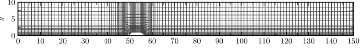
The geometry under consideration is a flat plate with an isolated roughness element placed at a finite distance from the leading edge. A schematic of the numerical domain and setup is shown in Fig. 1. The computational domain has periodic boundary conditions (BCs) at the spanwise boundaries, an isothermal no-slip condition at the wall, and characteristic boundary conditions at the top and outflow boundaries to avoid unwanted reflections. The flow is initialized with a compressible laminar similarity profile. This profile is normalized such that the laminar displacement thickness at the domain inflowδ 0 is unity and grows according to
δx^ δ 0 Δ 2Rex^ p Reδ 0 (10) with Rex^1 2 Re δ 0 Δ 2 Reδ 0 x δ 0 (11) (cf. [26]), wherex^ is the dimensional streamwise coordinate in a reference frame starting from the plate leading edge; andΔis a
BC
BC
BC Fig. 1 Schematic of the numerical domain used in the DNS, illustrating the position of the isolated roughness element and the applied boundary conditions.
scaling factor, dependent on Mach number and wall temperature, which is equal toΔ9.071in the current work. The Reynolds number based on the inflow displacement thickness is Reδ
0 14;000. The inflow is specified, with the exception of the pressure (which is linearly extrapolated from inside the domain in the subsonic region of the boundary layer, whereas in the supersonic region of the inflow, all the flow variables are fixed).
Different types of forcing can be used to trigger instabilities in the boundary layer, e.g., freestream turbulence, boundary-layer blowing and suction, entropy spots, acoustic waves, etc. Since it was shown in work by De Tullio [15] that acoustic disturbances are more effective than vortical or entropy disturbances at generating boundary-layer instabilities, acoustic disturbances are introduced in the freestream in the present study, with a source placed at streamwise and wall-normal positionsxf12.0andyf6.0according to
sx; t aexp−r2X M m0 XN n1 cosβmzϕmsinωntϕn (12) with amplitudeaand coordinaterqx−xf2 y−yf2. The spanwise wave number is defined asβm2πm∕Lz, and frequency is
ωn2πnF0withF00.02. The acoustic source has a broadband spectrum with M20 spanwise modes and N20 temporal modes to mimic the broadband nature of acoustic fluctuations originating from turbulent boundary layers, commonly present on wind-tunnel walls during experiments. The lower and upper bounds of the frequency and spanwise wave number range of the forcing govern, respectively, the simulation integration time of statistical quantities and the required grid resolution. The upper bound is selected so that the smallest wavelength of the forcing can be adequately resolved on the computational grid, whereas the lower bound is selected so as to limit the computational expense of the simulations. Random phasesϕmandϕnare introduced to avoid large
spikes in the imposed forcing. The acoustic disturbances are implemented by adding the forcing termsto the continuity equation. An isolated roughness element is placed at the domain’s spanwise centerline, with the roughness center located at a distancexr53
from the inflow, corresponding toRex^
r 1.933×10
6based on a reference frame starting from the plate leading edge. The roughness elements investigated are continuous (i.e., described by a smooth analytical function), such that a single-block body-fitted grid can be used. To ensure sufficient grid points near the roughness element, while keeping the computational expense reasonable, the numerical grid is stretched in the streamwise and spanwise directions. The grid consists of regions of constant grid spacing (a fine grid near the roughness element and a coarser grid near the domain boundaries) connected by ninth-order polynomials, such that the stretching function isC4continuous. In the wall-normal direction, the grid is stretched to ensure the boundary layer is sufficiently resolved. The stretching function between the uniform computational grid (0<η<1) and the nonuniform physical grid (y0<y<Ly) is given
by
yy0 Ly−y0
sinhbyη
sinhby (13)
wherebyis the stretching factor.
The details of the numerical domain and grid are summarized in Table 1. Note that the computational setup, except for the roughness shape and number of grid points, was taken to be the same as the setup of De Tullio and Sandham [10]. The grid size was taken to be at least as fine as their grid, for which a comprehensive grid study was performed. The current grid also contains more grid points in each direction than the grid used in the comparable Mach 6 simulations of Redford et al. [7]. For cases where transition is observed, the worst cases areΔx6.5,Δz7.0, andΔy<1.2for the first cell above the wall. Note that these values are computed at a location with a localized peak in friction velocity, and most of the values are well below these worst-case values.
A sketch of the computational mesh at the roughness centerline is shown in Fig. 2a to illustrate the grid stretching along the domain, and another is shown in Fig. 2b to illustrate the body-fitted grid around the (flat-top) roughness elements.
D. Characterization of the Roughness Element
Two elemental roughness shapes are considered: the smooth bump used in the work of Redford et al. [7] and a roughness shape with a more flattened top, using a definition very similar to the roughness of Marxen and Iaccarino [5]. The former roughness element is defined as y0x;~ z~ −c1 tanh x~ 2z~2 p c2 −1 tanh − ~ x2z~2 p c2 −1 (14) wherey0is theycoordinate of the grid point at the wall. In this equation,x~andz~are the coordinates relative to the roughness center. In these equations,c1andc2are defined as
c1c3 2 1cos j Ny π ; c2c4 1c5 j−1 Ny−1
withNyas the number of grid points in the wall-normal direction, j1;2; : : : Ny, and the constantsc30.6565,c42.28478, and c56. The constants are defined so as to have a roughness height of
k1.0 and a frontal area of Syz6.0. A three-dimensional
visualization of the roughness element, and its projection on thexy
andzyplanes, is shown in Fig. 3a.
To quantify the effect of the roughness shape on transition, a different function defining the roughness geometry is used that gives direct control on the slope of the roughness element’s sides, its width, and its maximum height. This function is defined as
y0x~ − k 2 tanhSW∕k × tanh S k 2 ~x−W tanh S k−2 ~x−W (15) wherekis the roughness height atx~0, andWis defined as the distance between the spanwise locations with the maximum slope.S
is defined asScotS, withSin the range0<S<π∕2. The variableScan be seen as a smoothness factor, which controls the slope of the roughness sides. In the limit ofS→0, the roughness becomes a sharp-edged element with 90 deg sides, that is the same as the“pizza-box”roughness element of De Tullio and Sandham [10]; whereas for increasingly large values of S, the roughness will become more smooth and bumplike. In the current work, the smoothness factor is set toSπ∕4andW6.0, except where mentioned otherwise. Note that the roughness type that follows from this formula will be called a flat-top roughness element hereafter.
Flat-top roughness elements with different planform shapes can be obtained by combination or modification of this roughness function. For example,y0r~with the radius from the roughness centerr~
~ x2y~2 p
will result in a cylindrical roughness element. The product
Table 1 Details of the computational grid
Parameter Value Lx×Ly×Lz 300×20×50 Nx×Ny×Nz 2415×205×468 ystretchingby 3.19 Δxa [0.15, 0.05, 0.135] Δzb [0.04, 0.15]
aValues of Δxindicate the grid spacing upstream, near the roughness and
downstream.
bValue ofΔzindicates that the grid is finer in the region near the roughness.
of y0x~ and y0z~, with x~ and z~ denoting the streamwise and spanwise coordinates relative to the roughness center, yields a roughness element with a square planform. Rotating the flat-top square 45 deg and scaling its width by a factor ofp2yields the flat-top roughness element with a diamond-shaped planform. Cylindrical flat-top roughness elements with heights ofk1.0andk0.5are visualized in Figs. 3b and 3c, respectively.
A third type of roughness element (namely, ramped up or ramped down) has been investigated. These roughness elements are a combination of the smooth bump and flat-top definition in the streamwise direction, whereas the flat-top definition is used in the spanwise direction. The rampup case is defined as a smooth bump element (withc46.85434) forx~≤0and a flat-top element for
~
x >0: and vice versa for the rampdown case. Three-dimensional visualizations of the rampup and rampdown roughness elements are shown in Figs. 3d and 3e, respectively.
E. Details of the Simulated Cases
Details of the 10 simulated roughness cases are given in Table 2. The naming of the roughness cases follows the following convention. The first letter signifies the wall temperature. Note that, in the current work, only hot wall (denoted H) results are discussed, and the wall temperature Tw for these cases is set to the adiabatic wall
temperature. The symbol after this first letter indicates the roughness shape: smooth bump (⊗), cylindrical (○), square (□), or diamond-shaped (⋄) flat-top roughness elements; and the rampup and rampdown elements are indicated by△and , respectively. The flat-top roughness element with heightk0.5 is indicated with the symbol•, and the flat-top with width W3.0is indicated with the symbol . Note that these symbols are also used as markers in the figures of this work to allow for an easy distinction between the results of different cases. The number that follows the roughness shape designation indicates the roughness heightk. Except for the a) Stretched grid in streamwise and wall-normal direction. Note that only every 10th grid line is shown
b) Close-up of the grid around the roughness elements
Fig. 2 Sketch of the computational grid.
Fig. 3 Three-dimensional visualizations of the roughness elements in the numerical simulations.
case with small flat-top roughness element , all cases have a roughness height ofk1.0. The last part of the naming represents the amplitude of imposed acoustic forcing introduced in Eq. (12): Ae5 for an amplitude of a6×10−5, and Ae4 fora6×10−4.
III. Results of Direct Numerical Simulations
A. Roughness-Induced Base Flow Modifications
To study the effect of the different roughness elements on transition, it needs to be understood how the different roughness elements affect the base flow. In this section, the roughness-induced base flow modifications that can influence the transition behavior are discussed.
1. Shear Layers and Recirculation Regions
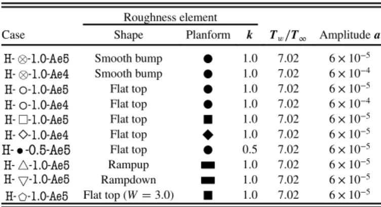
Figure 4 shows how the roughness shape, height, and planform change the shear layers around and behind the roughness element, using contours of wall-normal shear∂u∕∂yin the left-hand figures and shear magnitudeus, defined as
us≔ ∂u ∂y 2 ∂u ∂z 2 s (16) in the right-hand figures. Since it is the shear layers that can support the growth of convective instabilities, it is the difference in shear-layer structure and strength that is expected to yield the difference of transition behavior. The recirculation regions around the roughness elements are indicated in Fig. 4 using dashed contour lines of small negative velocity (i.e., u−1×10⁻⁵), and the length of these separated regions is summarized in Table 3.
Figures 4a and 4c show the shear layers around the smooth bump and cylindrical flat-top roughness elements, respectively. At the roughness centerline (left-hand figures), the recirculation region upstream of the flat top is larger, whereas the recirculation region downstream is of the same length. Also, the value of the wall-normal shear stress downstream of the roughness element (e.g., atx80) is
similar between the smooth bump and flat top, albeit thinner and further away from the wall behind the flat top. From the right-hand figures, the structure of the detached shear layer behind the flat top can be seen to be more curved and concentrated, and the high shear regions can be seen close to the wall (atz≈23andz≈25), generated by streamwise vorticity, and are considerably weaker behind the smooth bump.
The small flat-top roughness element (withk0.5) yields very weak shear layers compared to the flat-top element with a height of
k1.0, as can be seen by comparing Figs. 4b and 4c (right-hand figures). The strength and structure of the detached shear layer is more similar to the smooth bump (withk1.0), shown in Fig. 4a; therefore, the effect of these two roughness elements on the transition behavior is expected to be similar.
The effect of the planform of the roughness element can be observed by looking at Figs. 4c–4e, which show the shear layers for the cylindrical, square, and diamond-shaped flat-top roughness elements, respectively. From these figures, it can be seen that the difference between the cylindrical and square roughness elements is small, whereas the diamond-shaped flat top generates a slightly more curved detached shear layer and stronger wall-normal shear at the roughness centerline. The recirculation regions downstream of the roughness elements can be seen to be highly dependent on the roughness planform: the diamond-shaped roughness element has the shortest recirculation region, followed by the cylindrical, and finally the square flat-top roughness element. The separation lengths around the cylindrical and square elements are, respectively, 42 and 87% larger upstream and 15 and 37% larger downstream compared to the diamond-shaped roughness element.
The effect of ramping up or down the roughness element is shown by Figs. 4f and 4g, which should be compared with the square flat-top case of Fig. 4d. It can be seen that ramping up does not greatly modify the shear layers downstream. The strength and wall-normal location of the wall-normal shear at the centerline are roughly the same, although the shear regions offcenter and near the wall are slightly weaker. The recirculation region downstream of the rampup element is slightly larger, whereas upstream, no recirculation region is present due to the more gentle change in geometry.
In the case of the rampdown element, the flow upstream of the roughness behaves the same as the square flat-top element, whereas a large effect downstream can be observed. The downstream recirculation region has disappeared completely, which allows the detached shear layer to spread out and be brought closer to the wall, resulting in lower levels of wall-normal shear. The offcenter near-wall high-shear regions do not seem to be affected by ramping up or down, which would indicate that the streamwise vorticity generated by the roughness element is not weakened by the ramped-down aft section of the roughness element.
The effect of the roughness width or aspect ratio can be seen in Fig. 4h, which shows the case withW3.0and can be compared to the square flat-top element withW6.0in Fig. 4d. The shear layer downstream of the narrower roughness element is stronger and more concentrated. The recirculation regions around theW3.0element
Table 2 Details of the computational cases in the current work
Roughness element
Case Shape Planform k Tw∕T∞ Amplitudea Smooth bump 1.0 7.02 6×10⁻⁵ Smooth bump 1.0 7.02 6×10⁻⁴ Flat top 1.0 7.02 6×10⁻⁵ Flat top 1.0 7.02 6×10⁻⁴ Flat top 1.0 7.02 6×10⁻⁵ Flat top 1.0 7.02 6×10⁻⁵ Flat top 0.5 7.02 6×10⁻⁵ Rampup 1.0 7.02 6×10⁻⁵ Rampdown 1.0 7.02 6×10⁻⁵ Flat top (W3.0) 1.0 7.02 6×10⁻⁵
Table 3 Lengths of the separated regions upstream and downstream of the roughness elements
Case Lupsep Ldownsep
2.7 11.2 4.4 11.3 5.8 13.4 3.1 9.8 1.7 4.8 — 14.6 5.8 — 3.3 5.7
are approximately 43% (upstream) and 57% (downstream) shorter than those around the flat top withW6.0.
2. Vortical Structures
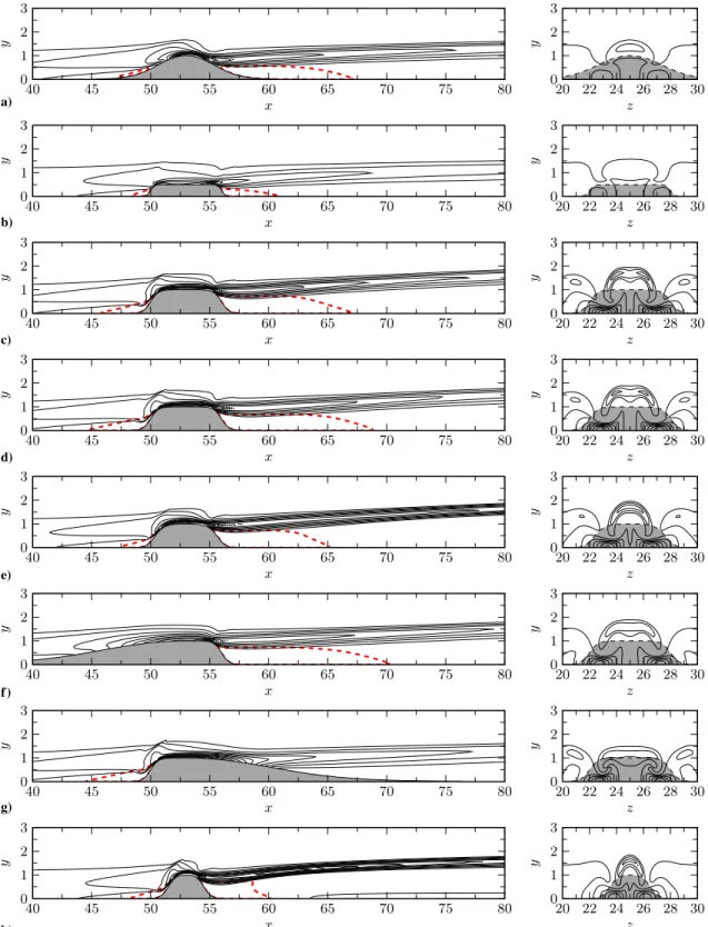
The vortical flow structures generated around the roughness elements are shown in Fig. 5, visualized by isosurfaces of the second invariant of the velocity gradient tensor (i.e., theQcriterion [27]) defined for compressible flow as
Q1 2 ∂ ui ∂xi 2 −∂ui ∂xj ∂uj ∂xi (17)
and colored by the local streamwise velocity. The recirculation regions are shown using black isosurfaces, which give a better understanding of the three-dimensional shape of the separation around the roughness elements.
From Fig. 5a, it can be seen that the smooth bump does not produce strong vortical structures downstream of the roughness. This is consistent with the relatively low spanwise shear stress in its wake, as observed in the previous section. A relatively large high-speed structure can be seen on top of the smooth bump, but this does not seem to have much influence on the downstream flow structures. The flow around the small roughness element of a) b) c) d) e) f ) g) h)
Fig. 4 Wall-normal shear∂u∕∂yat the domain centerline (left); shear magnitudeusatx85.0(right).
case is very similar to the smooth bump case, as shown in Fig. 5b.
The planform does not seem to have a dramatic effect on the structures around the flat-top roughness elements, as shown in Figs. 5c–5e. Upstream of the roughness, a low-speed horseshoe vortex can be seen to wrap itself around the elements. Stronger vortices are generated at the aft section of the elements in a high-speed flow region. These structures initially follow the shape of the downstream recirculation regions and become aligned in the streamwise direction further downstream. Because of the much narrower recirculation region behind the diamond-shaped roughness elements, this pair of streamwise-aligned vortices are located closer together than in the case of the cylindrical or square flat-top roughness element. The high-speed rollers generated on top, shown in Figs. 5c–5e, have a shape that is platform dependent, but this structure does not seem to have an effect on the downstream flow structures.
In the case of the rampup element, shown in Fig. 5f, no horseshoe vortex is generated. Similar to the flat-top element without a ramp, a strong streamwise-aligned vortex pair is generated downstream with a similar strength and spanwise position. Therefore, the flow structures downstream do not seem to be affected very much by the upstream rampup, and it is mainly the geometry of the roughness aft section that governs the flow structures in the roughness wake. This is confirmed by looking at the rampdown element in Fig. 5g. The flow structures at the front of the rampdown roughness (i.e., horseshoe vortex, high-speed roller on top) are almost identical to the square flat-top element without a ramp, as shown in Fig. 5d. However, the structures downstream of the rampdown are considerably affected. The streamwise-aligned vortex pair seems to be thinner and have a higher local streamwise velocity, indicating that the streamwise velocity deficit behind the rampdown roughness
element is much lower than the flat-top element without a downward ramp.
B. Roughness Effect on Transition
1. Prediction of Roughness-Induced Transition
Traditionally, a transition criterion based on roughness height has been used to separate the transitional and nontransitional cases. One of the most commonly used roughness-induced transition criteria is the roughness Reynolds numberRekk[18] defined as
Rekk≔ ukρkk
μk (18)
where uk, ρk, and μk are, respectively, the streamwise velocity,
density, and dynamic viscosity at the location and heightkof the roughness in an unperturbed boundary layer. This approach does not take into account the shape, planform, or background noise levels, yielding a range of critical Reynolds numbersRekkreported in the
literature. Variations ofRekk, where variables are taken at different
locations (either at the wall or the roughness height), are occasionally used, such as
Rekw≔ ukρkk
μw
(19)
[9], but neither of these solve the inherent limitations of this type of transition criterion. More recently, Bernardini et al. [19] proposed a new transition criterion based on momentum deficit due to the roughness elementReQdefined as
Fig. 5 Top view of the vortical ow structures, visualized by isosurfaces ofQ0.003.
ReQ≔ QS−yz1∕2
μw
(20) for which they found the critical value for bypass transition to occur at
ReQ>200−280for a wide range of roughness shapes. In their
work, they imposed a single forcing field at the inlet (i.e., random velocity fluctuations of a maximum of 0.5% of the freestream velocity) and noted the potential dependency of the critical value of
ReQon the type and level of the disturbance environment. In Eq. (20), Q≈ρkkDukFshape (21)
is the estimated momentum deficit, where
Fshape
Z1 0
ηwηdη (22)
withηy∕k, andwη wy∕D. In these equations,S
yzis the
projected frontal area andDis the diameter of the roughness element. Equation (20) can also be expressed as
ReQRekwD∕k1∕2Fshape (23)
which is the equation used to computeReQin the current work. This
criterion, being based on the (estimated) momentum deficit, takes into account to some degree the frontal shape of the roughness element.
The values ofRekk,Rekw, andReQfor the cases currently under
investigation are given in Table 4. The values ofRekkandReQare
also placed in the transition maps in Fig. 6, proposed by Redford et al. [7] and Bernardini et al. [19]. Note that the shaded regions in these maps are the proposed supercritical regions; i.e., the cases that lie in this region are expected to go through transition, whereas the others do not. It can be seen that all cases, except the flat-top roughness element with smaller height k0.5, are expected to trip the boundary layer and induce transition.
2. Transition Onset Location
The location at which transition is said to occur is not unambiguous. Different parameters can be looked at to determine the location of the point where the transition process starts, such as the boundary-layer intermittency or the skin-friction coefficientcf. It is
commonly said that an abrupt rise in skin friction signifies the start of the transition from a laminar to a turbulent boundary layer. However, how to quantify this rise and how to set an appropriate threshold is not straightforward, and changing these parameters could result in significantly different computed transition onset locations.
In the current work, the transition onset locationxtris defined as the first streamwise coordinate downstream of the roughness element such that the rate of increase of the skin-friction coefficient,
c0
fx dcf∕dx, is larger than (or equal to) 2% of the value of the
local skin-friction coefficientcfx, i.e.,
xtr≔x c0 fx cfx≥0.02 (24)
for which the values are computed at the roughness centerline. This definition is chosen because it consistently gives a reasonable estimate for the start of the skin-friction rise, determined visually by
a) Redford et al. [7] b) Bernardini et al. [19]
Fig. 6 Transition maps proposed by Redford et al. [7] and Bernardini et al. [19]. Symbols as per Table 2. Table 4 Computed transition Reynolds numbersRekk,
Rekw, andReQof the computational cases and geometric
parameters of the roughness elements in the current work
Case Rekk Rekw ReQ 984 728 618 984 728 793 984 728 793 984 728 758 127 119 135 984 728 793 984 728 793 984 728 516
Fig. 7 Skin-friction coefficient along the domain centerline. Line symbols as per Table 2.
the skin-friction plots in this section. This criterion does break down near the edges of flow reversal regions, wherecf0, however.
The skin-friction coefficient along the domain centerline is plotted in Fig. 7 for all cases with low (quiet) freestream disturbances (cases
Ae5). The dashed line in this figure shows the skin friction for a flat plate without a roughness element, and the filled diamond symbols indicate the transition onset location detected by the criterion in Eq. (24). It should be noted that the results shown in this section are time-averaged results with an averaging period equal to the imposed freestream forcing period. From Fig. 7, it can be seen that only
cases , , , , and
trigger a clear transition to turbulence, whereas cases
, , and remain laminar within
the computational domain. This is unexpected, since only roughness withk0.5(case ) would be laminar according to the predictions based onRekk,Rekw, andReQ.
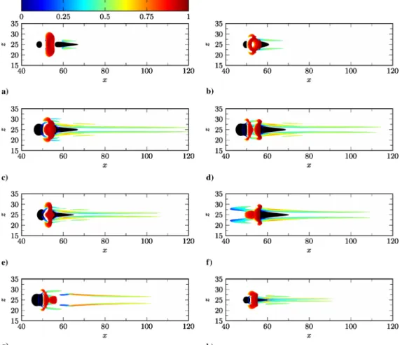
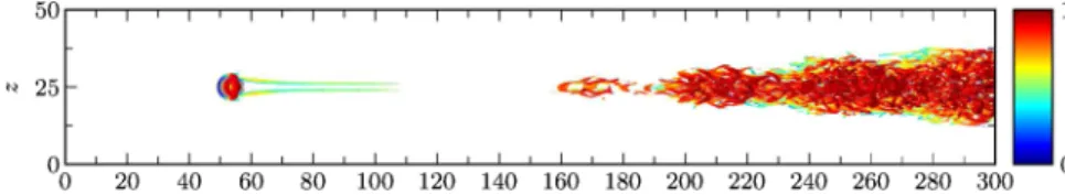
A visual impression of the transition process and the breakdown of the roughness wake can be seen in Fig. 8, which shows isosurfaces of
Q0.005 colored by the local streamwise velocity for case . Nearx≈160, hairpinlike vortices can be seen to form in the wake of the roughness element, which are quickly followed by the generation of a turbulent wedge starting from x≈190. By comparison with Fig. 7, it can be observed that this point corresponds to the location at which the skin-friction rise occurs, and thus the computed transition onset location.
For the cases that go through transition, the transition onset location lies at approximatelyxtr180−215, corresponding to 127−162 inflow displacement thicknesses downstream of the roughness. The computed transition onset locations for all cases are summarized in Table 5. The diamond-shaped roughness element seems to be the planform shape that is the most effective at inducing early transition, followed by the cylindrical and square flat-top elements. It is interesting to note that, between these three cases, the case with the smallest aft recirculation region has the earliest transition point, whereas the case with the largest aft recirculation region has the transition onset point furthest downstream. The aspect ratio does not seem to have a large effect on transition, since the difference between transition onset locations of cases
and is Δxtr≈3.3. This is a very small difference, considering the method used for the transition detection. Ramping up the square flat-top roughness element (i.e., as in case ) does not seem to promote earlier transition but shows a
small transition delay. However, even though the roughness element in case is ramped up, the recirculation region upstream of the square flat top acts as an effective ramp. The recirculation actually has a steeper effective ramp angle, as can be deduced from Fig. 4. Therefore, a ramped-up roughness element might still be more effective at promoting transition, but the effect would be very dependent on the actual shape and angle of the ramp.
As mentioned before, the smooth bump and rampdown roughness elements were not expected to remain laminar. Even though the smooth bump has the same height and frontal projected area as the flat-top roughness elements, the less abrupt change in geometry and the absence of large recirculation regions yields a less unstable roughness wake and early transition is not induced. This seems in slight contradiction to the Mach 6 smooth bump simulations of Redford et al. [7], who did see transition at a comparable Reynolds number. However, the acoustic disturbances they introduced in the freestream had an amplitude approximately 26 times larger than those in the current work. Since they also found a slight dependency of the transition onset location on the disturbance amplitude, the smooth bump in the current work might still induce transition within the computational domain in the presence of disturbances with higher amplitude. The effect of the freestream disturbance environment is investigated in the next section.
Especially, the aft part of the roughness seems to be of great importance, demonstrated by the rampdown case. The frontal profiles and the flow around the front part of the rampdown and square flat-top roughness elements are the same, as demonstrated by Figs. 4 and 5. However, the rampdown at the aft section promotes attached flow and allows for the detached shear layer to spread and weaken, resulting in very different behavior of the roughness wake and subsequent transition. This observation suggests that the streamwise profile and, in particular, the geometry of the aft section are of significant importance in the prediction of roughness-induced transition. However, this characteristic is not taken into consideration in any of the commonly used engineering correlations.
3. Freestream Disturbance Environment
So far, the effect of the freestream disturbance environment has not
been discussed. Cases and have,
respectively, a smooth bump and a cylindrical flat-top roughness element, but they have higher-amplitude disturbances imposed in the freestream, i.e., a noisier freestream. The amplitude in these cases is one order of magnitude greater than the reference cases
and .
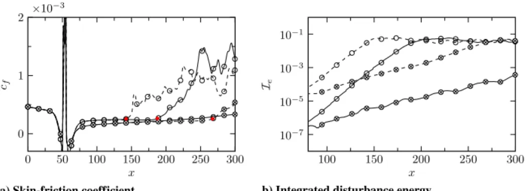
By increasing the disturbance level in the freestream, the smooth bump does start transition near the end of the numerical domain, as can be seen in Fig. 9a. In the case of the flat-top roughness element, the transition onset location moves forward approximately 45 inflow displacement thicknesses to xtr142.1. The amplitude of the disturbances in the noisy cases is still small enough to yield initially linear disturbances. The receptivity process is also linear, such that an increase of disturbance amplitude in the freestream of one order of magnitude translates into an increase of disturbance amplitude in the boundary layer of one order magnitude larger. This can be seen in Fig. 9b, which shows the disturbance energy, defined as
eu0u0v0v0w0w0 (25) integrated over the boundary-layer 99% thickness, evaluated at the roughness centerline. Figure 9b shows that the boundary-layer
Fig. 8 Top view of the breakdown into a turbulent wedge for case , shown by isosurfaces ofQ0.005using the local streamwise velocity.
Table 5 Computed transition onset locationxtr, maximum streak amplitudeAmaxst , and growth rateσdownstream of the
roughness elements Case xtr Amax st σ100<x<140 — 0.315 0.045 267.3 0.314 0.043 187.4 0.585 0.111 142.1 0.575 0.108 201.1 0.546 0.101 179.9 0.561 0.106 — 0.225 0.045 215.6 0.548 0.092 — 0.437 0.048 204.4 0.474 0.071
disturbances grow exponentially and their growth rate is not greatly dependent on the freestream disturbance environment. The growth of instabilities is, however, very dependent on the roughness element, as the wake generated by the flat-top roughness element is clearly more unstable than the wake behind the smooth bump. After the region of exponential disturbance growth, the disturbance energy can be seen to reach a saturation limit for the cases going through transition. This saturation signifies the occurrence of nonlinear interactions [15], which precede the breakdown to turbulence. It can thus be said that the transition onset location is shifted forward due to the linear receptivity process, and not due to a structurally modified transition process.
C. Roughness Wake Instability
To develop better predictions of roughness-induced transition, the mechanisms governing the transition need to be better understood. A mechanism-based approach would need to take into account the freestream flow conditions, disturbance environment, and roughness shape. Since it has been shown here that the streamwise roughness profile and, in particular, the aft section can have a large influence on the transition process, the full three-dimensional roughness shape needs to be considered, which is a characteristic not regarded in the commonly used transition prediction correlations. In this section, the correlation of the instability growth rate with several measures of the liftup effect due to the roughness elements is considered.
1. Instability Growth Rate
Table 5 lists the exponential growth rates σ of the integrated disturbance energyIe. It should be noted that the computation of the
growth rate is sensitive to the choice of evaluation location. The growth rateσin Table 5 is computed as the average growth rate in the range100<x<140in order to minimize this uncertainty. Since the growth rate is computed from the integrated disturbance energy, it encompasses the growth of all the instability modes present in the wake. No differentiation is made here between the different instability mode types, like sinuous and varicose modes, as was done in work by De Tullio and Sandham [10]. Although the growth rate of
the individual modes may vary significantly along the wake, the methodology employed here ensures that the growth rate of the most unstable mode is captured at each location.
It can be seen that the growth rates in Table 5 are highly dependent on the type of roughness element, and that even roughness elements with the same frontal profile (and thus the same values ofRekk,Rekw,
and ReQ) can have significantly different growth rates. These
roughness Reynolds numbers have been able to separate laminar and turbulent cases for simplified roughness geometries with various degrees of success, but they have a very limited applicability for general, fully three-dimensional roughness shapes and cannot be used to predict the wake instability or subsequent location of transition. This is also evidenced by Fig. 10, which shows the inverse of the transition length againstReQand gives no clear indication of a
useful correlation between the two.
2. Prediction of Growth Rate and Transition
An important step in the development of a better roughness-induced transition prediction tool would be if a relation could be found between the disturbance growth rate and a macroscopic feature of the roughness element or the flow in the vicinity of the roughness. All the empirical roughness Reynolds numbers fail this test, since it has been shown that cases with the same values ofRekk,Rekw, and ReQcan have entirely different instability growth rates and transition
onset locations.
If a transient growth scenario is considered as the initial mechanism behind the transition induced by a three-dimensional isolated roughness element, a relation between the disturbance growth rate and transient growth characteristics is expected. Counter-rotating vortices generated behind the roughness element transport low-momentum fluid away from the wall at the center and high-momentum fluid toward the wall at the sides of the roughness wake. This liftup mechanism, proposed by Landahl [28], generates streamwise streaks that initially grow algebraically in strength followed by a slow decay due to viscous dissipation. This process is transient growth, and it has been studied extensively in the context of optimal growth and bypass transition, as reviewed by Reshotko [29].
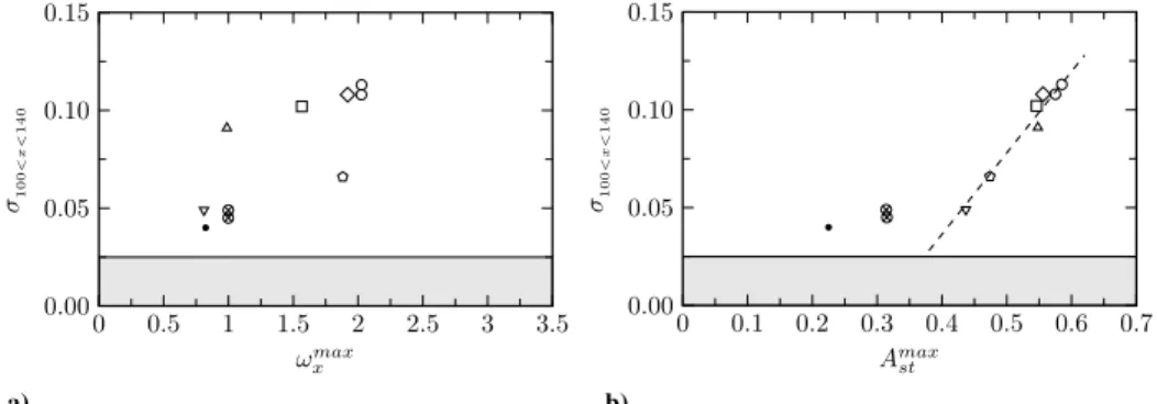
The generation of low- and high-momentum streaks has been observed behind the roughness elements for all the cases presented in the current work. Figure 11a shows the exponential disturbance growth rate plotted against the peak streamwise vorticity downstream of the roughness center, and it shows that stronger streamwise vorticity generated by the roughness element leads to a stronger liftup effect and, subsequently, a larger disturbance growth rate. The horizontal line separating the shaded region in this figure indicates the linear growth rate for a flat-plate boundary layer without a roughness element. The effect of counter-rotating streamwise vortices on liftup is clearly dependent on the vorticity magnitude, but it may also depend on the distance between the vortices, which is linked to the roughness element width. In contrast, the amplitude of the streak results directly from the liftup mechanism, and therefore is a metric that might give a trend independent of the roughness element geometry.
a) Skin-friction coefficient b) Integrated disturbance energy
Fig. 9 Eect of freestream disturbance level on skin friction and disturbance energy (solid: quiet; dashed: noisy).
Fig. 10 Inverse of the transition onset location plotted against the Reynolds number based on momentum deficitReQ. Symbols as per
Table 2.
The amplitude of a streak may be defined, using the formulation of Andersson et al. [30], as
Ast1
2maxy;z fu−ubg−miny;zfu−ubg (26)
whereubis the undisturbed laminar base flow. Andersson et al. [30]
investigated secondary instabilities of streaks in an incompressible boundary layer and found that streak instability occurs above a critical streak amplitude. They also showed a direct relationship between streak amplitude and growth rate of the streak instabilities (with a nonzero streamwise wave number). Table 5 lists the maximum streak amplitudes that are reached behind the roughness elements for all cases, and the computed growth rates are plotted against these values in Fig. 11b. From this figure, it is clear that a direct relationship between maximum streak amplitude and averaged growth rateσcan be observed, and that this correlation (at streak amplitudes greater than 0.4) seems to be stronger than the trend between the streamwise vorticity and growth rate. A linear regression line of the data points withAst>0.4is plotted in Fig. 11b, and it is defined as
σ0.416Amax
st −0.130 (27)
A minor dependency of the peak streak amplitude on the freestream disturbance level is apparent in Table 5 for cases and . It can be observed that the disturbance energy for noisy case reaches relatively high levels [i.e.,
O1%] at the location of peak streak amplitude in corresponding quiet case . Nonlinearities arise at these high levels and cause the streak to break down before the peak streak amplitude, obtained in the quiet case, is reached.
It should be noted that a consistent relation between the peak streak amplitude or growth rate and the transition onset location is not always found. In the near field of certain roughness elements, the disturbance levels might be more amplified, resulting in higher levels of disturbance energy and earlier transition onset, even if the exponential growth rate of the wake instabilities is slightly lower. This occurs for case , and it explains why this case has the earliest transition onset location but not the highest peak streak amplitude or disturbance growth rate.
If the trend between peak streak amplitude and average growth rate holds for a large range of roughness shapes and freestream parameters, the exponential growth rate downstream of the roughness element could be predicted by accurately determining the base flow and the resulting streak amplitude. The transition onset location would then be able to be predicted using anN-factor-type estimation, similar to the N-factor prediction of boundary-layer transition based on stability analysis, e.g., biglobal stability or analysis of the parabolized stability equations. An accurate description of this relation would then provide a mechanism-based prediction of roughness-induced transition without the need for stability analysis. The method proposed here gives an estimation of the average growth rate and does not predict variations in the streamwise direction, which can be estimated using stability analysis. Since this method requires
the streak amplitude, and thus the computation of the base flow near the roughness element, it would not be an a priori tool based only on the characteristics of the roughness element and the incoming boundary layer.
IV. Conclusions
Direct numerical simulations of Mach 6 flow over isolated roughness elements have been performed. A large variety of roughness shapes have been investigated, including a smooth bump, as well as cylindrical, square, diamond-shaped, and ramped-up/down roughness elements. It has been found that both the frontal profile and streamwise profile (in particular, the aft section of the roughness element) can greatly affect the growth of instabilities and, sub-sequently, the location of transition. The significance of the streamwise roughness profile on the transition onset is of great importance, since it is a characteristic that is not taken into account in any of the commonly used engineering correlations. The roughness element planform has been found to have a small influence on the transition onset location, with a diamond-shaped element being the most effective at inducing transition, followed by a cylindrical and square roughness element. A noisier acoustic disturbance envi-ronment is shown to bring transition forward due to a linear receptivity mechanism for the disturbance levels considered here. The generation of streamwise streaks is observed behind the roughness elements, and a direct relation between the maximum streak amplitude and exponential growth rate of instabilities in the roughness wake is found. This provides a step toward a mechanism-based approach to roughness-induced transition prediction mechanism-based on simulation of the local flow coupled to a stability analysis.
Acknowledgments
This work was performed within the Aerodynamic and Thermal Load Interactions with Lightweight Advanced Materials for High Speed Flight II project coordinated by European Space Agency-European Space Research and Technology Centre II is supported by the European Union within the 7th Framework Programme Theme 7 Transport, contract no. ACP0-GA-2010-263913. It made use of the facilities of HECToR, the United Kingdom’s national high-performance computing service, which is provided by UoE HPCx, Ltd., at the University of Edinburgh; Cray, Inc.; and Numerical Algorithms Group, Ltd., and it is funded by the Office of Science and Technology through Engineering and Physical Sciences Research Council’s High End Computing Programme. Computing time was provided by the U.K. Turbulence Consortium under Engineering and Physical Sciences Research Council grant EP/G069581/1.
References
[1] Reshotko, E., “Boundary-Layer Stability and Transition,” Annual
Review of Fluid Mechanics, Vol. 8, Jan. 1976, pp. 311–349.
doi:10.1146/annurev.fl.08.010176.001523
[2] McGinley, C. B., Berry, S. A., Kinder, G. R., Barnwell, M., Wang, K. C., and Kirk, B. S.,“Review of Orbiter Flight Boundary Layer Transition Data,” 9th AIAA/ASME Joint Thermophysics and Heat Transfer
a) b)
Fig. 11 Growth rate of integrated disturbance energy against a) the peak streamwise vorticity and b) the maximum streak amplitude.
Conference Proceedings, AIAA Paper 2006-2921, June 2006. doi:10.2514/6.2006-2921
[3] Berry, S. A., and Horvath, T. J.,“Discrete-Roughness Transition for Hypersonic Flight Vehicles,” Journal of Spacecraft and Rockets, Vol. 45, No. 2, 2008, pp. 216–227.
doi:10.2514/1.30970
[4] Schneider, S. P.,“Effects of Roughness on Hypersonic Boundary-Layer Transition,”Journal of Spacecraft and Rockets, Vol. 45, No. 2, 2008, pp. 193–209.
doi:10.2514/1.29713
[5] Marxen, O., and Iaccarino, G.,“Numerical Simulation of the Effect of a Roughness Element on High-Speed Boundary-Layer Instability,”38th
AIAA Fluid Dynamics Conference, AIAA Paper 2008-4400, 2008.
[6] Choudhari, M., Li, F., Wu, M., Chang, C., Edwards, J., Kegerise, M., and King, R., “Laminar-Turbulent Transition Behind Discrete Roughness Elements in a High-Speed Boundary Layer,”48th AIAA Aerospace Sciences Meeting Including the New Horizons Forum and
Aerospace Exposition, AIAA Paper 2010-1575, 2010.
[7] Redford, J. A., Sandham, N. D., and Roberts, G. T.,“Compressibility Effects on Boundary-Layer Transition Induced by an Isolated Roughness Element,”AIAA Journal, Vol. 48, No. 12, 2010, pp. 2818– 2830.
doi:10.2514/1.J050186
[8] Groskopf, G., Kloker, M. J., Stephani, K. A., Marxen, O., and Iaccarino, G.,“Hypersonic Flows with Discrete Oblique Surface Roughness and Their Stability Properties,” Center of Turbulence Research,
Proceedings of the Summer Program, Center for Turbulence Research,
Stanford, CA, 2010, pp. 1–17.
[9] Bernardini, M., Pirozzoli, S., and Orlandi, P.,“Compressibility Effects on Roughness-Induced Boundary Layer Transition,” International Journal of Heat and Fluid Flow, Vol. 35, 2012, pp. 45–51.
doi:10.1016/j.ijheatfluidflow.2012.02.007
[10] De Tullio, N., and Sandham, N. D.,“Influence of Boundary-Layer Disturbances on the Instability of a Roughness Wake in a High-Speed Boundary Layer,”Journal of Fluid Mechanics, Vol. 763, Jan. 2015, pp. 136–165.
doi:10.1017/jfm.2014.663
[11] Reshotko, E.,“Disturbances in a Laminar Boundary Layer Due to Distributed Surface Roughness,”Turbulence and Chaotic Phenomena in Fluids, edited by Tatsumi, T., Elsevier, Amsterdam, 1984, pp. 39–46. [12] Reshotko, E., and Tumin, A.,“Role of Transient Growth in Roughness-Induced Transition,”AIAA Journal, Vol. 42, No. 4, 2004, pp. 766–770. doi:10.2514/1.9558
[13] Groskopf, G., Kloker, M. J., and Marxen, O.,“Bi-Global Secondary Stability Theory for High-Speed Boundary-Layer Flows,”Center of
Turbulence Research, Proceedings of the Summer Program, Center for
Turbulence Research, Stanford, CA, 2008, pp. 1–18.
[14] Choudhari, M., Norris, A., Li, F., Chang, C.-L., and Edwards, J.,“Wake Instabilities Behind Discrete Roughness Elements in High Speed Boundary Layers,”51st AIAA Aerospace Sciences Meeting, AIAA Paper 2013-0081, 2013, pp. 1–17.
doi:10.2514/6.2013-81
[15] De Tullio, N.,“Receptivity and Transition to Turbulence of Supersonic Boundary Layers with Surface Roughness,” Ph.D. Thesis, Univ. of Southampton, Southampton, England, U.K., 2013.
[16] Wheaton, B. M., and Schneider, S. P.,“Roughness-Induced Instability in a Hypersonic Laminar Boundary Layer,”AIAA Journal, Vol. 50, No. 6, 2012, pp. 1245–1256.
doi:10.2514/1.J051199
[17] Subbareddy, P., Bartkowicz, M., and Candler, G.,“Direct Numerical Simulation of High-Speed Transition Due to an Isolated Roughness Element,”Journal of Fluid Mechanics, Vol. 748, June 2014, pp. 848– 878.
doi:10.1017/jfm.2014.204
[18] Reda, D. C., “Review and Synthesis of Roughness-Dominated Transition Correlations for Reentry Applications,” Journal of
Spacecraft and Rockets, Vol. 39, No. 2, 2002, pp. 161–167.
doi:10.2514/2.3803
[19] Bernardini, M., Pirozzoli, S., Orlandi, P., and Lele, S. K.,
“Parameterization of Boundary-Layer Transition Induced by Isolated Roughness Elements,”AIAA Journal, Vol. 52, No. 10, 2014, pp. 2261– 2269.
doi:10.2514/1.J052842
[20] Touber, E., and Sandham, N. D.,“Large-Eddy Simulation of Low-Frequency Unsteadiness in a Turbulent Shock-Induced Separation Bubble,” Theoretical and Computational Fluid Dynamics, Vol. 23, No. 2, 2009, pp. 79–107.
doi:10.1007/s00162-009-0103-z
[21] Carpenter, M., Nordström, J., and Gottlieb, D., “A Stable and Conservative Interface Treatment of Arbitrary Spatial Accuracy,”
Journal of Computational Physics, Vol. 148, No. 2, 1999, pp. 341–365.
doi:10.1006/jcph.1998.6114
[22] Wray, A. A.,“Very Low Storage Time-Advancement Schemes,”NASA Ames Research Center, Internal Rept., Moffet Field, CA, 1986. [23] Sandham, N. D., Li, Q., and Yee, H. C.,“Entropy Splitting for
High-Order Numerical Simulation of Compressible Turbulence,”Journal of
Computational Physics, Vol. 178, No. 2, 2002, pp. 307–322.
doi:10.1006/jcph.2002.7022
[24] Ducros, F., Ferrand, V., Nicoud, F., Weber, C., Darracq, D., Gacherieu, C., and Poinsot, T.,“Large-Eddy Simulation of the Shock/Turbulence Interaction,”Journal of Computational Physics, Vol. 152, No. 2, 1999, pp. 517–549.
doi:10.1006/jcph.1999.6238
[25] Yee, H. C., Sandham, N. D., and Djomehri, M. J.,“Low-Dissipative High-Order Shock-Capturing Methods Using Characteristic-Based Filters,”Journal of Computational Physics, Vol. 150, No. 1, 1999, pp. 199–238.
doi:10.1006/jcph.1998.6177
[26] White, F. M.,Viscous Fluid Flow, 2nd ed., McGraw–Hill, New York, 1991, pp. 504–508.
[27] Jeong, J., and Hussain, F.,“On the Identification of a Vortex,”Journal of Fluid Mechanics, Vol. 285, Feb. 1995, pp. 69–94.
doi:10.1017/S0022112095000462
[28] Landahl, M. T.,“A Note on an Algebraic Instability of Inviscid Parallel Shear Flows,” Journal of Fluid Mechanics, Vol. 98, No. 2, 1980, pp. 243–251.
doi:10.1017/S0022112080000122
[29] Reshotko, E., “Transient Growth: A Factor in Bypass Transition,”
Physics of Fluids, Vol. 13, No. 5, 2001, Paper 1067.
doi:10.1063/1.1358308
[30] Andersson, P., Brandt, L., Bottaro, A., and Henningson, D. S.,“On the Breakdown of Boundary Layer Streaks,”Journal of Fluid Mechanics, Vol. 428, Feb. 2001, pp. 29–60.
doi:10.1017/S0022112000002421
M. Choudhari
Associate Editor