K.B.M.Q. Zaman, S.M. Hirt, and T.J. Bencic
Glenn Research Center, Cleveland, Ohio
Boundary Layer Flow Control by an Array of
Ramp-Shaped Vortex Generators
NASA/TM—2012-217437
NASA STI Program . . . in Pro
fi
le
Since its founding, NASA has been dedicated to the advancement of aeronautics and space science. The NASA Scientifi c and Technical Information (STI) program plays a key part in helping NASA maintain this important role.
The NASA STI Program operates under the auspices of the Agency Chief Information Offi cer. It collects, organizes, provides for archiving, and disseminates NASA’s STI. The NASA STI program provides access to the NASA Aeronautics and Space Database and its public interface, the NASA Technical Reports Server, thus providing one of the largest collections of aeronautical and space science STI in the world. Results are published in both non-NASA channels and by NASA in the NASA STI Report Series, which includes the following report types:
• TECHNICAL PUBLICATION. Reports of completed research or a major signifi cant phase of research that present the results of NASA programs and include extensive data or theoretical analysis. Includes compilations of signifi cant scientifi c and technical data and information deemed to be of continuing reference value. NASA counterpart of peer-reviewed formal professional papers but has less stringent limitations on manuscript length and extent of graphic presentations.
• TECHNICAL MEMORANDUM. Scientifi c and technical fi ndings that are preliminary or of specialized interest, e.g., quick release reports, working papers, and bibliographies that contain minimal annotation. Does not contain extensive analysis.
• CONTRACTOR REPORT. Scientifi c and technical fi ndings by NASA-sponsored contractors and grantees.
• CONFERENCE PUBLICATION. Collected papers from scientifi c and technical
conferences, symposia, seminars, or other meetings sponsored or cosponsored by NASA. • SPECIAL PUBLICATION. Scientifi c,
technical, or historical information from NASA programs, projects, and missions, often concerned with subjects having substantial public interest.
• TECHNICAL TRANSLATION. English-language translations of foreign scientifi c and technical material pertinent to NASA’s mission. Specialized services also include creating custom thesauri, building customized databases, organizing and publishing research results.
For more information about the NASA STI program, see the following:
• Access the NASA STI program home page at http://www.sti.nasa.gov
• E-mail your question via the Internet to help@ sti.nasa.gov
• Fax your question to the NASA STI Help Desk at 443–757–5803
• Telephone the NASA STI Help Desk at 443–757–5802
• Write to:
NASA Center for AeroSpace Information (CASI) 7115 Standard Drive
K.B.M.Q. Zaman, S.M. Hirt, and T.J. Bencic
Glenn Research Center, Cleveland, Ohio
Boundary Layer Flow Control by an Array of
Ramp-Shaped Vortex Generators
NASA/TM—2012-217437
National Aeronautics and
Space Administration
Glenn Research Center
Cleveland, Ohio 44135
Acknowledgments
Support from the Subsonic Fixed Wing Project of the NASA Fundamental Aeronautics Program is gratefully acknowledged.
Available from NASA Center for Aerospace Information
7115 Standard Drive Hanover, MD 21076–1320
National Technical Information Service 5301 Shawnee Road Alexandria, VA 22312
Available electronically at http://www.sti.nasa.gov
This work was sponsored by the Fundamental Aeronautics Program at the NASA Glenn Research Center.
Level of Review: This material has been technically reviewed by technical management. Trade names and trademarks are used in this report for identifi cation
only. Their usage does not constitute an offi cial endorsement, either expressed or implied, by the National Aeronautics and
Boundary Layer Flow Control by an Array of
Ramp-Shaped Vortex Generators
K.B.M.Q. Zaman, S.M. Hirt, and T.J. Bencic National Aeronautics and Space Administration
Glenn Research Center Cleveland, Ohio 44135
Abstract
Flow field survey results for the effect of ramp-shaped vortex generators (VG) on a turbulent
boundary layer are presented. The experiments are carried out in a low-speed wind tunnel and the data are acquired primarily by hot-wire anemometry. Distributions of mean velocity and turbulent stresses as well as streamwise vorticity, on cross-sectional planes at various downstream locations, are obtained. These detailed flow field properties, including the boundary layer characteristics, are documented with the primary objective of aiding possible computational investigations. The results show that VG orientation with apex upstream, that produces a downwash directly behind it, yields a stronger pair of streamwise vortices. This is in contrast to the case with apex downstream that produces a pair of vortices of opposite sense. Thus, an array of VG’s with the former orientation, usually considered for film-cooling application, may also be superior for mixing enhancement and boundary layer separation control.
Introduction
The objective of this study is to obtain a database on the flowfield past an array of ramp-shaped vortex generators (VG) placed in a turbulent boundary layer. Each VG produces a pair of streamwise vortices. The series of vortices with alternating clockwise and counter-clockwise sense, produced by the array, enhance mixing in the boundary layer. This has the potential application for control of secondary flow and boundary layer separation. A tie-in of the present effort is with an experiment conducted earlier in the 8- by 6-Foot Supersonic Wind Tunnel at the NASA Glenn Research Center (Ref. 1). The study addressed flow control for an inlet using similar VG’s with the aim of alleviating shock-induced boundary layer separation. While the VG array in the latter experiment was designed with guidance from CFD studies and past experience with various shapes of VG’s (Refs. 2 and 3), questions remained regarding the optimum parameters. The focus of the present study, conducted in a low-speed wind tunnel, is to explore the optimum parameters of the VG array. Detailed data on the evolution of the flowfield properties are obtained while the spacing and orientation of the VG’s are varied. Most of the data are acquired for VG geometry such that there is an ‘upwash’ between the pair of vortices originating from it. This
configuration considered in the cited inlet experiment, as well as in References 2 and 3, will be referred to in the following as ‘VG-u’. A summary of the results obtained in the present study with this configuration has been given in a conference paper (Ref. 4). Subsequently, a limited parametric study was conducted with the reversed orientation of the VG’s—a configuration referred to as ‘VG-d’ in the following. The VG-d geometry, producing a ‘downwash’ between the pair of vortices, has been considered for film-cooling application (Refs. 5 and 6). Effects of the VG array with the two opposite orientations are compared and analyzed for otherwise identical conditions. Highlights of the results are discussed in the following text. All datasets on the flow-field properties including boundary layer characteristics, vorticity and turbulent stresses, usually difficult to measure at higher speeds, are also documented in order to aid possible CFD investigations. These datasets can be found on a supplemental CD (not published on the Web) which may be requested from the NASA Center for AeroSpace Information (CASI) at
http://www.sti.nasa.gov, or 443–757–5802. Further description of the data files are provided in the appendix at the end of this report.
NASA/TM—2012-217437 2
Experimental Procedure
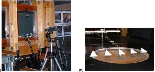
Flow-visualization and hot-wire anemometry experiments are conducted in a low speed, open-loop wind tunnel. A picture of the tunnel test section, set up for flow visualization, is shown in Figure 1(a). A picture of the VG array placed on the test section floor is shown in Figure 1(b); the flow is into the page and the VG orientation is such as to produce an upwash directly behind it (VG-u). Also seen in
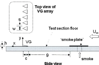
Figure 1(b) is the probe traversing mechanism with two crossed hot-wires. A schematic of the
experimental setup is given in Figure 2 illustrating various definitions as well as the coordinate system. An ‘array’ will imply 5 equally spaced VG’s placed in a line perpendicular to the tunnel flow. Note that the spacing (s) in the array is defined as the edge-to-edge distance and not the pitch of the repetitive pattern. In the following text, when the configuration is obvious the suffix ‘-u’ and ‘-d’ will be dropped from ‘VG-u’ or ‘VG-d’ for simplicity. All data pertain to a nominal tunnel velocity (U) of 29 ft/sec.
Flow visualization was performed using a Rosco (Rosco Laboratories, Stamford, CT) fog machine. Smoke was introduced through a hole in the tunnel floor into a narrow chamber, formed between the floor and a thin plate. Smoke came out as a sheet through the downstream slit of the chamber which was approximately 0.075 in. high and 6 in. wide. The location of the slit was about 9 in. upstream of the VG array. Thus, a sheet of smoke was simply introduced into the approach boundary layer, part of which got entrained by the streamwise vortices and marked the velocity defect region downstream of the VG’s. The cross-section of the flow field was visualized by a laser sheet and the data were recorded by a video camera; (an interested reader may find some further description of the set up and procedure in (Ref. 7)). Samples of the visualization pictures for various VG spacing and different x-locations are shown in the following but these are not included in the supplemental CD. For consistency all hot-wire measurements were performed with the smoke plate left in its place.
The two X-wire probes, one in u-v and another in u-w configuration, were used for flow-field surveys downstream of the array. They were stepped through the same grid points in space and thus
time-averaged values for all three components of velocity and turbulence intensity were acquired at each point. In addition, two components of Reynolds stress were obtained while from the velocities on y-z plane the streamwise component of vorticity (x) was calculated. A single hot-wire measurement provided the
boundary layer profiles at different x-locations on the center plane (z = 0) of the flow domain. The dimensions of each VG (in inches) were, w = 1.16, h = 0.561 and c = 1.435 (Fig. 2). The tunnel speed was U∞ = 29 ft/s yielding a Reynolds number based on the width w, Rew17,500. The
approach boundary layer momentum thickness was, 2 /w 0.08. In the following, the VG base width w
and the tunnel speed U∞ are used to nondimensionalize the data.
Results
Figure 3 shows laser sheet illuminated cross-section of the flow past an array of VG-u. The pictures in Figures 3(a) to (c) show the flow field at three streamwise locations for a given spacing, s/w = 0.5. The pictures in Figures 3(d) to (f) show the flow field at a given location (x/w = 2.1) for three additional VG spacing. The velocity defect due to individual VG’s can be seen clearly. With increasing streamwise distance (from pictures in Figures 3(a) to (c)) the smoke traces get more diffused. With increasing spacing (from Figures 3(d) to (f)) the velocity defects move farther from one another. Thus, with zero spacing in (d) the defect regions are almost merged together while with the largest spacing (s/w = 1) in (f) there is little interaction among the defect regions.
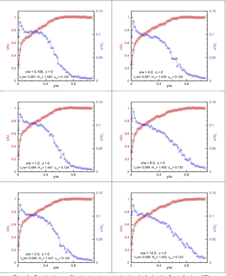
Figure 4 shows the tunnel boundary layer characteristics without any VG. The legends in each plot show the measurement location (x/w), momentum thickness (2 /w), shape factor (H12 = 1 /2, where 1 is
the displacement thickness)as well as the peak turbulence intensity (u’max /U). It can be seen that the momentum thickness grows gradually with increasing streamwise distance. The shape factor appears to show an inverse trend. The peak turbulence does not exhibit any clear trend and may be considered to
remain about the same. The boundary layer is inferred to be nominally turbulent throughout the measurement domain.
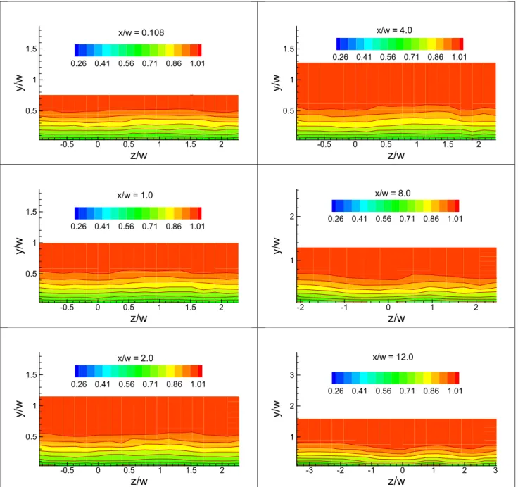
Figure 5 shows X-wire survey results for mean velocity on the y-z plane, without any VG, for the same x-locations of Figure 4. The velocity contours, especially at the farthest downstream locations, exhibit mild undulations possibly due to imperfections in the smoke plate (§2). Nevertheless, the
boundary layer may be considered two dimensional for the purposes of this study where gross distortions are introduced by the VG’s.
Before conducting detailed hot-wire surveys the effect of spatial resolution in the measurement was briefly checked at x/w = 1 for the flow over a single VG-u. The step size in z was varied while that in y
was held a constant at 0.08 inches. Mean velocity and streamwise vorticity measured for three z-step sizes are shown in Figure 6. It can be seen that the largest step size (0.22 in.) resulted in obviously smeared distributions while the other two step sizes essentially produced similar results. Thus, for this x-station the intermediate step size was chosen for further measurements. The step size was varied for other
streamwise locations (smaller upstream but larger downstream) based on past experience so that the smearing due to inadequate spatial resolution was minimal while data acquisition time in the surveys was not prohibitively long.
While the accompanying folder contains all data, only streamwise mean velocity, turbulence intensity and vorticity at limited locations are discussed in the following. Figure 7 shows the flow field properties for a single VG-u at two x/w locations. (The U and x data at x/w = 1 are repeat measurements (see
Fig. 6). The repetition in this and some later figures are made to facilitate a direct visual comparison). At
x/w = 1, the mean velocity distribution exhibits the typical ‘kidney’ shape. In this shape, the higher momentum fluid is on the top periphery while the interior holds lower momentum fluid drawn from the wall boundary layer. As already done while discussing the flow visualization pictures, the kidney shaped region will be alternatively referred to as the ‘velocity defect’ in the following. The maximum turbulence intensity occurs within it. The pair of streamwise vortices, originating from the VG, is also seen nestled within this region. At the downstream measurement location (x/w = 12) a dome of low momentum fluid with high turbulence marks the velocity defect, although turbulence is not as high as in the boundary layer. The streamwise vortex pair has diffused and is barely detectable.
The streamwise evolution of the flow field is captured by the mean velocity distributions in Figures 8 to 11, for VG-u spacing (s/w) of 0, 0.25, 0.5 and 1, respectively. As seen with the flow visualization, the velocity defects are closer together for smaller spacing (Fig. 8). By x/w = 8, these have merged together and at the last station the flow domain essentially has become a thick boundary layer. With the largest spacing (Fig. 11), on the other hand, there is little interaction and each velocity defect behaves as if it is from an isolated VG (compare with data in Fig. 7). For mixing enhancement within the boundary layer, perhaps, the preferred effect is an intermediate situation where the defects are neither too far apart nor completely merged together. Thus, for s/w = 0 (Fig. 8), for example, the most beneficial effect may be expected around x/w = 4. This implies that if boundary layer separation control is desired at a given location, a VG array with zero spacing should be placed about 4 widths upstream. With larger spacing the array needs to be placed farther upstream and the available extent of the flow in the actual hardware may thus dictate the choice of the VG configuration. Some further analysis and discussion of this issue is given in Reference 4.
Mean velocity, turbulence intensity and streamwise vorticity data are shown in Figure 12 for the effect of the VG-u array with zero spacing, as an example. The data, for two x/w locations, are presented in the same format as for the single VG-u case in Figure 7. (As stated before, some of the mean velocity plots are repeats to enable a direct visual comparison for the reader). Of note is the x distribution at the
downstream location. Even though the contours are diffused, significantly stronger positive and negative vortex structures can be seen on the left and right of the domain, respectively. The vorticity from the middle of the domain has migrated leaving barely detectable structures. When viewed at x/w = 12, it is as if the array of five VG’s acted as a single wider VG.
NASA/TM—2012-217437 4
Data for the reversed orientation of the vortex generators (VG-d) are now discussed and compared with corresponding data from VG-u arrays. Figure 13 shows data corresponding to Figure 12 for VG-d array with zero spacing. Note the shift in the positions of the velocity defect; while it was centered at
z = 0 in the left column in Figure 12, for example, two defect regions straddle z = 0 in Figure 13. This is because the signs of the vortex pair from the individual VG’s have switched. The latter is evident upon an inspection of the vorticity data at x/w = 1. The effect at x/w = 12 is by and large similar to that seen in Figure 12, however, there are subtle differences. One difference is that the streamwise vortices (displayed with the same scale in the two figures) are stronger especially at the downstream location, a point
elaborated further in the following.
Only the mean velocity distributions are compared for VG-u and VG-d arrays for different spacing, as shown in Figure 14. These data are for x/w = 1 and significant differences in the flow field are noticed for wider spacing. The effect of the VG-d array appears to pervade farther in span. Corresponding data at
x/w = 12 are compared in Figure 15. Upon a further scrutiny it can be seen that a more pronounced effect has persisted with the VG-d array with wider spacing. Thus, a stronger lifting of low momentum fluid from the boundary layer (blue contours) can be seen within the velocity defects for the VG-d case.
The turbulence intensity distributions for the VG-u and VG-d arrays are compared side by side in Figure 16 for s/w = 0 and 1 and x/w = 1 and 12, as indicated. Commensurate with the mean velocity data (Fig. 14), the turbulence intensity for the VG-d array with the wider spacing and at the upstream location (row 2), are seen to be more uniformly distributed. In comparison, the corresponding flow field for the VG-u array is marked by distinct velocity defect regions. At x/w = 12 the turbulence distributions have become somewhat similar for the two cases, although the intensities are somewhat higher for the VG-d case. Streamwise vorticity distribution, compared similarly in Figure 17, exhibits distinct differences at the downstream measurement station. The vortices are clearly stronger for the VG-d case. Peak
streamwise vorticity, taken as the average of the absolute values from the two in a pair, is only slightly larger at the upstream location for the VG-d case (2.84 versus 2.61 for s/w = 0; 3.15 versus 2.82 for
s/w = 1). Corresponding values at the downstream location for the VG-d case are more than double of that for the VG-u case. These trends are analyzed further in the following.
The peak vorticity (as defined in the previous paragraph) is plotted in Figure 18 as a function of x/w. For the VG-u arrays, the values are identical at the upstream locations. Farther downstream, the values appear to be somewhat larger with the array cases relative to the single VG-u case, however, there does not seem to be a consistent trend. For the VG-d arrays data were acquired only at x/w = 1 and 12. At either location, the peak x value was found to be affected little by the spacing. Average values at those
two locations for the VG-d case are shown by the solid square symbols. It can be seen that the peak vorticity value is slightly larger at the upstream location, however, it is significantly larger at the downstream location relative to the data for the VG-u cases. Thus, the vorticity produced and its persistence in the flow is clearly more pronounced for the VG-d configuration. This effect is further illustrated with the following data.
The streamwise vorticity magnitudes for the same ramp-shaped VG’s were measured earlier in connection with a film-cooling study (Ref. 6). The effect of the VG on an inclined jet-in-crossflow was explored. An issue addressed was the effect of the roundedness of the edges of the VG since, in
applications, sharp-edged VG’s may not always be practical. A series of VG’s were designed with increasing radius of curvature for the upper edges while keeping the frontal blockage to the flow a constant. This resulted in VG shapes shown by the pictures at the top of Figure 19—the limiting case being a hemisphere. The pertinent data are the peak streamwise vorticity measured at a fixed downstream location with the jet turned off and with the tunnel flow at the same speed as considered here. Peak x,
(defined the same way, i.e., average of the two absolute peaks from a pair), is shown in Figure 19. Value from a vortex pair with downwash sense is assigned a positive sign while that from a pair of upwash sense is assigned a negative sign. The data are presented as a function of the radius of curvature used to round off the edges of the VG, normalized by the radius of the limiting hemisphere case. Open data points are for the film-cooling (VG-d) configuration while the solid data points are for the opposite VG-u configuration. It can be seen that the absolute magnitudes of peak x are significantly larger in the VG-d
configuration. It is as if the flow favors the downwash sense, producing a pair of vortices of that sense even in the limiting hemispherical case (i.e., at the abscissa value of unity).
Figure 19 also shows that with increasing roundedness of the edges the vorticity magnitude drops off with either VG orientation. Thus, sharp edged VG’s are more effective even though small amount of roundedness may be quite acceptable in practice. What is important in the present context is the higher vorticity magnitude produced by the VG-d configuration. An array of VG’s with either orientation produces an array of streamwise vortices with alternating signs. However, the VG-d array produces an array of stronger vortices. Thus, the latter configuration may be preferable not only for film-cooling application but also for mixing enhancement and separation control for a boundary layer.
Conclusion
An array of VG’s may be used for control of secondary flow or separation of a boundary layer. The appropriate spacing of the VG’s should depend on the distance available between the location where the VG’s may be placed in the hardware and the location where flow separation is expected. At a given location downstream the impact of the VG array may be less if the spacing is too large. On the other hand, the impact may also be also less if the velocity defects from individual VG’s have already merged
together due to too short spacing. Thus, the optimum effect may occur when the velocity defects are about to merge by the time they arrive at the separation location. Following this criterion, the present data indicate that the VG spacing needs to be zero if the separation location is only about 4w away, 0.25w if the separation location is about 8w away, etc. An important inference is that the VG’s with apex
upstream, such that there is a downwash directly behind each, produce stronger streamwise vortices. This is in contrast to VG’s with opposite orientation considered in previous flow separation control studies. Thus, an array VG’s with the former orientation may be expected to be more effective not only for film-cooling application but also for boundary layer separation control.
Appendix—Data Files
The following is a description of the data files accompanying this TM. The data files can be found on a supplemental CD (not published on the Web) which may be requested from the NASA Center for AeroSpace Information (CASI) at http://www.sti.nasa.gov, or 443–757–5802.
(1) 5_VG-u_diff_spacings_all_surveys.—These are X-wire survey data for different VG spacing and for measurement at different streamwise location. The VG’s are oriented with apex downstream (VG-u). While examples of U, u’and x data are shown in the hardcopy, these data files also include v’, w’, uv and
uw (all nondimensionalized by freestream velocity (U) and VG base width (w)). [Notes: (1) Plot routines
are included for convenience; some shows nondimensionalization by the symbol ‘d’ which should be replaced by ‘w’. (2) In the files, U is represented by ‘ubv’, u’ by ‘ur’, v’ by ‘vr’, w’ by ‘wr’ and x by
‘wx’.]
(2) 5VG-d_0w_apart_film_cool_config.—These are X-wire survey data for ‘VG-d’ array with spacing of s = 0. Each VG is placed with apex upstream so that there is a ‘downwash’ between the pair of streamwise vortices. Other comments as in item 1 apply.
(3) 5VG-d_diff_s_x_1_x_12.—These are X-wire survey data for ‘VG-d’ array at 2 streamwise locations for different spacing. Other comments as in item 1 apply.
(4) Boundary_layer_profiles_diff_x.—These data are taken by a single hot-wire. Columns 1, 2 and 3 are y/w, U/U and u'/U, respectively. Boundary layer momentum thickness (2), shape factor (H12) and
maximum turbulence intensity (u’max) are noted in the last line.
(5) Misc_line_plots.—These are data files for various line plots at end of TM. The peak streamwise vorticity is the average of the absolute values of the two counter-rotating components in the pair. For explanation of VG edge roundedness see the TM.
(6) No_VG_U_surveys_diff_x.—These are survey data for mean velocity for the baseline flow without any VG.
(7) survey_at_x_1_to_check_grid_density_effect.—These are X-wire survey data assessing the effect of survey grid resolution. The vertical step size (in y) is kept constant at 0.08 inches while the horizontal step (in z) size is varied as 0.22, 0.11 and 0.055 inches for 'course', 'medium' and 'fine' cases, respectively. Other comments as in item 1 apply.
(8) survey_single_VG_x_1_and_12.—These are X-wire survey data for a single VG at two streamwise stations. Other comments as in item 1 apply.
(a) (b)
Figure 1.—Experimental facility. (a) Wind tunnel test section and set-up for flow visualization. (b) Interior of test section showing VG array and hot-wires.
NASA/TM—2012-217437 8
Figure 2.—Schematic of experimental set-up.
(a) s = 0.5, x0.9 (d) s = 0.0, x2.1 (b) s = 0.5, x2.1 (e) s = 0.25, x2.1 (c) s = 0.5, x3.9 (f) s = 1.0, x2.1
Figure 3.—Laser-sheet illuminated cross-section of the flow field. (a)-(c): streamwise evolution of flow for array of 5 VG with spacing s/w = 0.5; (d)-(f): flow at a fixed streamwise location for array of 5 VG with different spacing.
Figure 4.—Boundary layer profiles at various streamwise locations for the baseline flow (without any VG). y/w U/ U u' /U 0 0.4 0.8 0 0.2 0.4 0.6 0.8 1 0 0.05 0.1 0.15 x/w = 0.108, z = 0 2/w= 0.081 H12= 1.462 umx= 0.126 y/w U/ U u' /U 0 0.4 0.8 0 0.2 0.4 0.6 0.8 1 0 0.05 0.1 0.15 x/w = 4.0, z = 0 2/w= 0.087 H12= 1.435 umx= 0.128 y/w U/ U u' /U 0 0.4 0.8 0 0.2 0.4 0.6 0.8 1 0 0.05 0.1 0.15 x/w = 1.0, z = 0 2/w= 0.084 H12= 1.447 umx= 0.124 y/w U/ U u' /U 0 0.4 0.8 0 0.2 0.4 0.6 0.8 1 0 0.05 0.1 0.15 x/w = 8.0, z = 0 2/w= 0.089 H12= 1.405 umx= 0.130 y/w U/ U u' /U 0 0.4 0.8 0 0.2 0.4 0.6 0.8 1 0 0.05 0.1 0.15 x/w = 2.0, z = 0 2/w= 0.085 H12= 1.437 umx= 0.125 y/w U/ U u' /U 0 0.4 0.8 0 0.2 0.4 0.6 0.8 1 0 0.05 0.1 0.15 x/w = 12.0, z = 0 2/w= 0.096 H12= 1.402 umx= 0.123
NASA/TM—2012-217437 10
Figure 5.—Mean velocity (U/U) distribution at different x for the baseline flow (without VG). z/w y/w -0.5 0 0.5 1 1.5 2 0.5 1 1.5 0.26 0.41 0.56 0.71 0.86 1.01 x/w = 0.108 z/w y/w -0.5 0 0.5 1 1.5 2 0.5 1 1.5 0.26 0.41 0.56 0.71 0.86 1.01 x/w = 4.0 z/w y/w -0.5 0 0.5 1 1.5 2 0.5 1 1.5 0.26 0.41 0.56 0.71 0.86 1.01 x/w = 1.0 z/w y/w -2 -1 0 1 2 1 2 0.26 0.41 0.56 0.71 0.86 1.01 x/w = 8.0 z/w y/w -0.5 0 0.5 1 1.5 2 0.5 1 1.5 0.26 0.41 0.56 0.71 0.86 1.01 x/w = 2.0 z/w y/w -3 -2 -1 0 1 2 3 1 2 3 0.26 0.41 0.56 0.71 0.86 1.01 x/w = 12.0
U U U w x Course (0.08 0.2 2) Medium (0.08 0.1 1) Fine (0.08 0.0 55)
Figure 6.—Effect of measurement grid resolution on mean velocity and streamwise vorticity distribution at x/w = 1; data are for a single VG with ‘upwash’ orientation (VG-u).
z/w y/w -0.5 -0.25 0 0.25 0.5 0 0.5 0.26 0.41 0.56 0.71 0.86 1.01 z/w y/w -0.5 0 0.5 0 0.5 -2.50 -1.32 0.26 1.44 2.62 3.80 z/w y/w -0.5 -0.25 0 0.25 0.5 0 0.5 0.26 0.41 0.56 0.71 0.86 1.01 z/w y/w -0.5 0 0.5 0 0.5 -2.50 -1.32 0.26 1.44 2.62 3.80 z/w y/w -0.5 -0.25 0 0.25 0.5 0 0.5 0.26 0.41 0.56 0.71 0.86 1.01 z/w y/w -0.5 0 0.5 0 0.5 -2.50 -1.32 0.26 1.44 2.62 3.80
NASA/TM—2012-217437 12 x/w = 1 x/w = 12 U U U u' U w x
Figure 7.—Mean velocity, turbulence intensity and streamwise vorticity at two x-locations for the flow past a single VG-u.
z/w y/w -1 -0.5 0 0.5 1 0.5 1 1.5 0.40 0.52 0.64 0.77 0.89 1.01 z/w y/w -2 -1.5 -1 -0.5 0 0.5 1 1.5 0.5 1 1.5 2 0.60 0.68 0.76 0.84 0.92 1.00 z/w y/w -1 -0.5 0 0.5 1 0 0.5 1 0.00 0.03 0.06 0.09 0.12 0.15 z/w y/w -2 -1.5 -1 -0.5 0 0.5 1 1.5 0.5 1 1.5 2 0.00 0.02 0.04 0.05 0.07 0.09 z/w y/w -1 -0.5 0 0.5 1 0 0.5 1 -1.73 -0.73 0.27 1.28 2.28 3.28 z/w y/w -2 -1.5 -1 -0.5 0 0.5 1 1.5 0.5 1 1.5 2 -0.12 -0.08 -0.04 0.04 0.08 0.12
Figure 8.—Streamwise evolution of mean velocity (U/U) for the array of 5 VG-u with spacing s/w = 0. z/w y/w -0.5 0 0.5 1 1.5 2 0.5 1 1.5 0.26 0.41 0.56 0.71 0.86 1.01 x/w = 0.108 z/w y/w -1 -0.5 0 0.5 1 1.5 2 0.5 1 1.5 2 0.65 0.72 0.79 0.87 0.94 1.01 x/w = 4 z/w y/w -0.5 0 0.5 1 1.5 2 0.5 1 1.5 0.40 0.52 0.64 0.77 0.89 1.01 x/w = 1 z/w y/w -2 -1.5 -1 -0.5 0 0.5 1 1.5 2 2.5 0.5 1 1.5 2 2.5 0.60 0.68 0.76 0.85 0.93 1.01 x/w = 8 z/w y/w -0.5 0 0.5 1 1.5 2 0.5 1 1.5 0.55 0.64 0.73 0.83 0.92 1.01 x/w = 2 z/w y/w -3 -2 -1 0 1 2 3 1 2 3 0.62 0.70 0.78 0.85 0.93 1.01 x/w = 12
NASA/TM—2012-217437 14
Figure 9.—Streamwise evolution of mean velocity (U/U) for the array of 5 VG-u with spacing s/w = 0.25. z/w y/w -0.5 0 0.5 1 1.5 2 0.5 1 1.5 0.26 0.41 0.56 0.71 0.86 1.01 x/w = 0.108 z/w y/w -1 -0.5 0 0.5 1 1.5 2 0.5 1 1.5 2 0.65 0.72 0.79 0.87 0.94 1.01 x/w = 4 z/w y/w -0.5 0 0.5 1 1.5 2 0.5 1 1.5 0.40 0.52 0.64 0.77 0.89 1.01 x/w = 1 z/w y/w -2 -1.5 -1 -0.5 0 0.5 1 1.5 2 2.5 0.5 1 1.5 2 2.5 0.60 0.68 0.76 0.85 0.93 1.01 x/w = 8 z/w y/w -0.5 0 0.5 1 1.5 2 0.5 1 1.5 0.55 0.64 0.73 0.83 0.92 1.01 x/w = 2 z/w y/w -3 -2 -1 0 1 2 3 1 2 3 0.62 0.70 0.78 0.85 0.93 1.01 x/w = 12
Figure 10.—Streamwise evolution of mean velocity (U/U) for the array of 5 VG-u with spacing s/w = 0.5. z/w y/w -0.5 0 0.5 1 1.5 2 0.5 1 1.5 0.26 0.41 0.56 0.71 0.86 1.01 x/w = 0.108 z/w y/w -1 -0.5 0 0.5 1 1.5 2 0.5 1 1.5 2 0.65 0.72 0.79 0.87 0.94 1.01 x/w = 4 z/w y/w -0.5 0 0.5 1 1.5 2 0.5 1 1.5 0.40 0.52 0.64 0.77 0.89 1.01 x/w = 1 z/w y/w -2 -1.5 -1 -0.5 0 0.5 1 1.5 2 2.5 0.5 1 1.5 2 2.5 0.60 0.68 0.76 0.85 0.93 1.01 x/w = 8 z/w y/w -0.5 0 0.5 1 1.5 2 0.5 1 1.5 0.55 0.64 0.73 0.83 0.92 1.01 x/w = 2 z/w y/w -3 -2 -1 0 1 2 3 1 2 3 0.62 0.70 0.78 0.85 0.93 1.01 x/w = 12
NASA/TM—2012-217437 16
Figure 11.—Streamwise evolution of mean velocity (U/U) for the array of 5 VG-u with spacing s/w = 1. z/w y/w -0.5 0 0.5 1 1.5 2 0.5 1 1.5 0.26 0.41 0.56 0.71 0.86 1.01 x/w = 0.108 z/w y/w -1 -0.5 0 0.5 1 1.5 2 0.5 1 1.5 2 0.65 0.72 0.79 0.87 0.94 1.01 x/w = 4 z/w y/w -0.5 0 0.5 1 1.5 2 0.5 1 1.5 0.40 0.52 0.64 0.77 0.89 1.01 x/w = 1 z/w y/w -2 -1.5 -1 -0.5 0 0.5 1 1.5 2 2.5 0.5 1 1.5 2 2.5 0.60 0.68 0.76 0.85 0.93 1.01 x/w = 8 z/w y/w -0.5 0 0.5 1 1.5 2 0.5 1 1.5 0.55 0.64 0.73 0.83 0.92 1.01 x/w = 2 z/w y/w -3 -2 -1 0 1 2 3 1 2 3 0.62 0.70 0.78 0.85 0.93 1.01 x/w = 12
x/w = 1 x/w = 12 U U U u' U w x
Figure 12.—Mean velocity, turbulence intensity and streamwise vorticity distributions at two x-locations for the array of 5 VG-u with spacing s/w = 0. z/w y/w -0.5 0 0.5 1 1.5 2 0.5 1 1.5 0.40 0.52 0.64 0.77 0.89 1.01 x/w = 1 z/w y/w -3 -2 -1 0 1 2 3 1 2 3 0.62 0.70 0.78 0.85 0.93 1.01 x/w = 12 z/w y/w -0.5 0 0.5 1 1.5 2 0.5 1 1.5 0.00 0.03 0.06 0.09 0.12 0.15 x/w = 1 z/w y/w -3 -2 -1 0 1 2 3 1 2 3 0.00 0.02 0.04 0.05 0.07 0.09 x/w = 12 z/w y/w -0.5 0 0.5 1 1.5 2 0.5 1 1.5 -1.74 -0.74 0.25 1.24 2.23 3.22 x/w = 1 z/w y/w -3 -2 -1 0 1 2 3 1 2 3 -0.16 -0.11 -0.06 0.02 0.07 0.12 x/w = 12
NASA/TM—2012-217437 18 U U U u' U w x
Figure 13.—Mean velocity, turbulence intensity and streamwise vorticity distributions at two x-locations for the array of 5 VG-d with spacing s/w = 0; VG-d is VG with reversed orientation producing a ‘downwash’ directly behind.
z/w y/w -0.5 0 0.5 1 1.5 2 0.5 1 1.5 0.40 0.52 0.64 0.77 0.89 1.01 x/w = 1 z/w y/w -3 -2 -1 0 1 2 3 1 2 3 0.62 0.70 0.78 0.85 0.93 1.01 x/w = 12 z/w y/w -0.5 0 0.5 1 1.5 2 0.5 1 1.5 0.00 0.03 0.06 0.09 0.12 0.15 x/w = 1 z/w y/w -3 -2 -1 0 1 2 3 1 2 3 0.00 0.02 0.04 0.05 0.07 0.09 x/w = 12 z/w y/w -0.5 0 0.5 1 1.5 2 0.5 1 1.5 -1.74 -0.74 0.25 1.24 2.23 3.22 x/w = 1 z/w y/w -3 -2 -1 0 1 2 3 1 2 3 -0.16 -0.11 -0.06 0.02 0.07 0.12 x/w = 12
VG-u VG-d s/w = 0 s/w = 0.25 s/w = 0.5 s/w = 1
Figure 14.—Comparison of mean velocity distributions at x/w = 1 for the array of VG’s with different spacing. Left column for ‘upwash’ orientation (VG-u) and right column for ‘downwash’ (film-cooling) orientation of vortex generator (VG-d).
z/w y/ w -0.5 0 0.5 1 1.5 2 0.5 1 1.5 0.40 0.52 0.64 0.77 0.89 1.01 x/w = 1 z/w y/ w -0.5 0 0.5 1 1.5 2 0.5 1 1.5 0.40 0.52 0.64 0.77 0.89 1.01 x/w = 1 z/w y/ w -0.5 0 0.5 1 1.5 2 0.5 1 1.5 0.40 0.52 0.64 0.77 0.89 1.01 x/w = 1 z/w y/ w -0.5 0 0.5 1 1.5 2 0.5 1 1.5 0.40 0.52 0.64 0.77 0.89 1.01 x/w = 1 z/w y/ w -0.5 0 0.5 1 1.5 2 0.5 1 1.5 0.40 0.52 0.64 0.77 0.89 1.01 x/w = 1 z/w y/ w -0.5 0 0.5 1 1.5 2 0.5 1 1.5 0.40 0.52 0.64 0.77 0.89 1.01 x/w = 1 z/w y/ w -0.5 0 0.5 1 1.5 2 0.5 1 1.5 0.40 0.52 0.64 0.77 0.89 1.01 x/w = 1 z/w y/ w -0.5 0 0.5 1 1.5 2 0.5 1 1.5 0.40 0.52 0.64 0.77 0.89 1.01 x/w = 1
NASA/TM—2012-217437 20 VG-u VG-d s/w = 0 s/w = 0.25 s/w = 0.5 s/w = 1
Figure 15.—Comparison of mean velocity distributions at x/w = 12 for the array of VG’s with different spacing. Left column for ‘upwash’ orientation (VG-u) and right column for ‘downwash’ orientation of vortex generator (VG-d).
z/w y/ w -3 -2 -1 0 1 2 3 1 2 3 0.62 0.70 0.78 0.85 0.93 1.01 x/w = 12 z/w y/ w -3 -2 -1 0 1 2 3 1 2 3 0.62 0.70 0.78 0.85 0.93 1.01 x/w = 12 z/w y/ w -3 -2 -1 0 1 2 3 1 2 3 0.62 0.70 0.78 0.85 0.93 1.01 x/w = 12 z/w y/ w -3 -2 -1 0 1 2 3 1 2 3 0.62 0.70 0.78 0.85 0.93 1.01 x/w = 12 z/w y/ w -3 -2 -1 0 1 2 3 1 2 3 0.62 0.70 0.78 0.85 0.93 1.01 x/w = 12 z/w y/ w -3 -2 -1 0 1 2 3 1 2 3 0.62 0.70 0.78 0.85 0.93 1.01 x/w = 12 z/w y/ w -3 -2 -1 0 1 2 3 1 2 3 0.62 0.70 0.78 0.85 0.93 1.01 x/w = 12 z/w y/ w -3 -2 -1 0 1 2 3 1 2 3 0.62 0.70 0.78 0.85 0.93 1.01 x/w = 12
VG-u VG-d s/w = 0 x/w = 1 s/w = 1 x/w = 1 s/w = 0 x/w = 12 s/w = 1 x/w = 12
Figure 16.—Comparison of turbulence intensity at x/w = 1 and 12 for s/w = 0 and 1, as indicated. Left column for ‘upwash’ orientation (VG-u) and right column for ‘downwash’ orientation of vortex generator (VG-d).
z/w y/ w -0.5 0 0.5 1 1.5 2 0.5 1 1.5 0.00 0.03 0.06 0.09 0.12 0.15 x/w = 1 z/w y/ w -0.5 0 0.5 1 1.5 2 0.5 1 1.5 0.00 0.03 0.06 0.09 0.12 0.15 x/w = 1 z/w y/ w -0.5 0 0.5 1 1.5 2 0.5 1 1.5 0.00 0.03 0.06 0.09 0.12 0.15 x/w = 1 z/w y/ w -0.5 0 0.5 1 1.5 2 0.5 1 1.5 0.00 0.03 0.06 0.09 0.12 0.15 x/w = 1 z/w y/ w -3 -2 -1 0 1 2 3 1 2 3 0.00 0.02 0.04 0.05 0.07 0.09 x/w = 12 z/w y/ w -3 -2 -1 0 1 2 3 1 2 3 0.00 0.02 0.04 0.05 0.07 0.09 x/w = 12 z/w y/ w -3 -2 -1 0 1 2 3 1 2 3 0.00 0.02 0.04 0.05 0.07 0.09 x/w = 12 z/w y/ w -3 -2 -1 0 1 2 3 1 2 3 0.00 0.02 0.04 0.05 0.07 0.09 x/w = 12
NASA/TM—2012-217437 22 VG-u VG-d s/w = 0 x/w = 1 s/w = 1 x/w = 1 s/w = 0 x/w = 12 s/w = 1 x/w = 12
Figure 17.—Comparison of streamwise vorticity at x/w = 1 and 12 for s/w = 0 and 1, as indicated. Left column for ‘upwash’ orientation (VG-u) and right column for ‘downwash’ orientation of vortex generator (VG-d).
z/w y/ w -0.5 0 0.5 1 1.5 2 0.5 1 1.5 -1.74 -0.74 0.25 1.24 2.23 3.22 x/w = 1 z/w y/ w -0.5 0 0.5 1 1.5 2 0.5 1 1.5 -1.74 -0.74 0.25 1.24 2.23 3.22 x/w = 1 z/w y/ w -0.5 0 0.5 1 1.5 2 0.5 1 1.5 -1.74 -0.74 0.25 1.24 2.23 3.22 x/w = 1 z/w y/ w -0.5 0 0.5 1 1.5 2 0.5 1 1.5 -1.74 -0.74 0.25 1.24 2.23 3.22 x/w = 1 z/w y/ w -3 -2 -1 0 1 2 3 1 2 3 -0.16 -0.11 -0.06 0.02 0.07 0.12 x/w = 12 z/w y/ w -3 -2 -1 0 1 2 3 1 2 3 -0.16 -0.11 -0.06 0.02 0.07 0.12 x/w = 12 z/w y/ w -3 -2 -1 0 1 2 3 1 2 3 -0.16 -0.11 -0.06 0.02 0.07 0.12 x/w = 12 z/w y/ w -3 -2 -1 0 1 2 3 1 2 3 -0.16 -0.11 -0.06 0.02 0.07 0.12 x/w = 12
Figure 18.—Peak streamwise vorticity versus x for different VG cases as indicated; xmax is the average of absolute peak values in the two components of the vortex pair.
Figure 19.—Effect of varying roundedness of the outer edges of the VG on peak streamwise vorticity at x/w 6.5 (Ref. 5). * * x / w xma x w/ U 0 2 4 6 8 10 12 1 2 3 4 5 Single VG-u s/w = 1 s/w = 0.5 s/w = 0.25 s/w = 0 VG-d average *
Radius of curvature of VG edges
X w/ U -peak 0 0.2 0.4 0.6 0.8 1 -0.5 0 0.5 1 VG-d ('downwash' configuration)
References
1. Hirt, S.M., Chima, R.V., Vyas, M.A., Wayman, T.R., Conners, T.R., and Reger, R.W., “Experimental Investigation of a Large-Scale Low-Boom Inlet Concept,” AIAA Paper 2011-3796, 29th AIAA Applied Aerodynamics Conf., Jun 27-30, Honolulu, Hawaii.
2. Hirt, S.M. and Anderson, B.H., “Experimental investigation of the application of microramp flow control to an oblique shock interaction,” AIAA Paper 2009-919, 47th Aerospace Sciences Meeting, January 5-8, Orlando, FL.
3. Ford, C.W.P., and Babinsky, H., “Micro-Ramp Control of Oblique Shock Wave/Boundary Layer Interactions,” 37th Fluid Dynamics Conference, AIAA Paper 2007-4115, June 2007.
4. Hirt, S.M., Zaman, K.B.M.Q., and Bencic, T.J., “Experimental study of boundary layer flow control by an array of ramp-shaped vortex generators,” AIAA Paper 2012-0741, 50th Aerospace Sciences Meeting,
January 9-12, Nashville, TN.
5. Rigby, D.L., and Heidmann, J.D., “Improved Film Cooling Effectiveness by Placing a Vortex Generator Downstream of Each Hole,” ASME Gas Turbine Conference, American Society of Mechanical Engineers Paper 2008-GT-51361, Fairfield, NJ, June 2008.
6. Zaman, K.B.M.Q., Rigby, D.L., and Heidmann, J.D., “Inclined Jet in Crossflow Interacting with a Vortex Generator,” 2010, J. Prop. And Power, 26(5), September, pp. 947-954.
7. Milanovic, I.M., Zaman, K.B.M.Q., and Bencic, T.J., “Unsteady wake vortices in jets in cross flow,” DOI 10.1007/s12650-011-0114-x, Journal of Flow Visualization, 2011.
REPORT DOCUMENTATION PAGE OMB No. 0704-0188Form Approved
The public reporting burden for this collection of information is estimated to average 1 hour per response, including the time for reviewing instructions, searching existing data sources, gathering and maintaining the data needed, and completing and reviewing the collection of information. Send comments regarding this burden estimate or any other aspect of this collection of information, including suggestions for reducing this burden, to Department of Defense, Washington Headquarters Services, Directorate for Information Operations and Reports (0704-0188), 1215 Jefferson Davis Highway, Suite 1204, Arlington, VA 22202-4302. Respondents should be aware that notwithstanding any other provision of law, no person shall be subject to any penalty for failing to comply with a collection of information if it does not display a currently valid OMB control number.
PLEASE DO NOT RETURN YOUR FORM TO THE ABOVE ADDRESS.
1. REPORT DATE(DD-MM-YYYY)
01-04-2012 2. REPORT TYPETechnical Memorandum 3. DATES COVERED(From - To)
4. TITLE AND SUBTITLE
Boundary Layer Flow Control by an Array of Ramp-Shaped Vortex Generators
5a. CONTRACT NUMBER 5b. GRANT NUMBER
5c. PROGRAM ELEMENT NUMBER 6. AUTHOR(S)
Zaman, K.B.M.Q.; Hirt, S., M.; Bencic, T., J.
5d. PROJECT NUMBER 5e. TASK NUMBER 5f. WORK UNIT NUMBER
WBS-561581.02.08.03.47.06.03
7. PERFORMING ORGANIZATION NAME(S) AND ADDRESS(ES)
National Aeronautics and Space Administration John H. Glenn Research Center at Lewis Field Cleveland, Ohio 44135-3191
8. PERFORMING ORGANIZATION REPORT NUMBER
E-18130
9. SPONSORING/MONITORING AGENCY NAME(S) AND ADDRESS(ES)
National Aeronautics and Space Administration Washington, DC 20546-0001 10. SPONSORING/MONITOR'S ACRONYM(S) NASA 11. SPONSORING/MONITORING REPORT NUMBER NASA/TM-2012-217437 12. DISTRIBUTION/AVAILABILITY STATEMENT Unclassified-Unlimited Subject Categories: 02 and 07
Available electronically at http://www.sti.nasa.gov
This publication is available from the NASA Center for AeroSpace Information, 443-757-5802 13. SUPPLEMENTARY NOTES
A CD-ROM containing the supplemental data files mentioned in the Introduction section of this report can be requested from the NASA Center for AeroSpace Information at http://www.sti.nasa.gov, or 443-757-5802.
14. ABSTRACT
Flow field survey results for the effect of ramp-shaped vortex generators (VG) on a turbulent boundary layer are presented. The experiments are carried out in a low-speed wind tunnel and the data are acquired primarily by hot-wire anemometry. Distributions of mean velocity and turbulent stresses as well as streamwise vorticity, on cross-sectional planes at various downstream locations, are obtained. These detailed flow field properties, including the boundary layer characteristics, are documented with the primary objective of aiding possible
computational investigations. The results show that VG orientation with apex upstream, that produces a downwash directly behind it, yields a stronger pair of streamwise vortices. This is in contrast to the case with apex downstream that produces a pair of vortices of opposite sense. Thus, an array of VG’s with the former orientation, usually considered for film-cooling application, may also be superior for mixing enhancement and boundary layer separation control.
15. SUBJECT TERMS
Vortex generators; Vorticity dynamics; Turbulence
16. SECURITY CLASSIFICATION OF: 17. LIMITATION OF ABSTRACT UU 18. NUMBER OF PAGES 31
19a. NAME OF RESPONSIBLE PERSON
STI Help Desk (email:[email protected])
a. REPORT U b. ABSTRACT U c. THIS PAGE U
19b. TELEPHONE NUMBER (include area code) 443-757-5802
Standard Form 298 (Rev. 8-98) Prescribed by ANSI Std. Z39-18