The copyright © of this thesis belongs to its rightful author and/or other copyright owner. Copies can be accessed and downloaded for non-commercial or learning purposes without any charge and permission. The thesis cannot be reproduced or quoted as a whole without the permission from its rightful owner. No alteration or changes in format is allowed without permission from its rightful owner.
MODIFICATION OF
S
1STATISTIC WITH HODGES-LEHMANN
AS THE CENTRAL TENDENCY MEASURE
LEE PING YIN
MASTER OF SCIENCE (STATISTICS)
UNIVERSITI UTARA MALAYSIA
i
Permission to Use
In presenting this thesis in fulfilment of the requirements for a postgraduate degree from Universiti Utara Malaysia, I agree that the University’s Library may make it freely available for inspection. I further agree that permission for the copying of this thesis in any manner, in whole or in part, for scholarly purpose may be granted by my supervisor(s) or, in their absence, by the Dean of Awang Had Salleh Graduate School of Arts and Sciences. It is understood that any copying or publication or use of this thesis or parts thereof for financial gain shall not be allowed without my written permission. It is also understood that due recognition shall be given to me and to Universiti Utara Malaysia for any scholarly use which may be made of any material from my thesis.
Requests for permission to copy or to make other use of materials in this thesis, in whole or in part, should be addressed to:
Dean of Awang Had Salleh Graduate School of Arts and Sciences UUM College of Arts and Sciences
Universiti Utara Malaysia 06010 UUM Sintok
ii
Abstrak
Andaian kenormalan dan kehomogenan varians adalah merupakan perkara penting bagi prosedur parametrik seperti dalam pengujian kesamaan kecendurangan memusat. Sebarang ketidakpatuhan andaian tersebut boleh meningkatkan kadar Ralat Jenis I yang serius, yang akan mengakibatkan penolakan hipotesis nol yang tidak betul. Prosedur parametric seperti ANOVA dan ujian-t sangat bergantung pada andaian yang sukar ditemui dalam data sebenar. Sebaliknya, prosedur tak berparameter tidak bergantung pada taburan data tetapi prosedur tersebut kurang kuasanya. Untuk mengatasi isu yang dinyatakan, prosedur teguh adalah dicadangkan. Statistik S1 adalah salah satu prosedur teguh yang menggunakan median sebagai parameter lokasi untuk menguji kesamaan kecenderungan memusat di antara kumpulan, dan ia membabitkan data asal tanpa perlu memangkas atau mentransformasi data untuk mencapai kenormalan. Kajian terdahulu terhadap S1 menunjukkan kekurangan keteguhan dalam beberapa keadaan di bawah reka bentuk seimbang. Oleh itu, objektif kajian ini adalah menambahbaik statistik S1 asal dengan menggantikan median kepada penganggar Hodges-Lehmann. Penggantian juga dilakukan terhadap penganggar skala menggunakan varians bagi penganggar
Hodges-Lehmann serta beberapa penganggar skala teguh yang lain. Bagi memeriksa kekuatan dan kelemahan prosedur yang dicadangkan dalam mengawal Ralat Jenis I, beberapa pemboleh seperti jenis taburan, bilangan kumpulan, saiz kumpulan yang seimbang dan tidak seimbang, varians yang sama dan tidak sama, dan sifat pasangan telah dimanipulasikan. Hasil kajian menunjukkan kesemua prosedur yang dicadangkan adalah teguh merentasi semua keadaan bagi setiap kes kumpulan. Selain itu, tiga prosedur yang dicadangkan iaitu S1(MADn), S1(Tn) dan S1(Sn) menunjuk prestasi yang lebih baik berbanding prosedur S1 asal di bawah taburan pencong yang ekstrem. Secara keseluruhan, prosedur yang dicadangkan menunjukkan keupayaannya mengawal peningkatan Ralat Jenis I. Oleh yang demikian, objektif kajian ini telah tercapai apabila tiga daripada prosedur yang dicadangkan menunjukkan peningkatan keteguhan di bawah taburan terpencong.
Katakunci: Statistik S1, Hodges-Lehmann, penganggar skala teguh, ralat Jenis I,
iii
Abstract
Normality and variance homogeneity assumptions are usually the main concern of parametric procedures such as in testing the equality of central tendency measures. Violation of these assumptions can seriously inflate the Type I error rates, which will cause spurious rejection of null hypotheses. Parametric procedures such as ANOVA and t-test rely heavily on the assumptions which are hardly encountered in real data. Alternatively, nonparametric procedures do not rely on the distribution of the data, but the procedures are less powerful. In order to overcome the aforementioned issues, robust procedures are recommended. S1 statistic is one of the robust procedures which uses median as the location parameter to test the equality of central tendency measures among groups, and it deals with the original data without having to trim or transform the data to attain normality. Previous works on S1 showed lack of robustness in some of the conditions under balanced design. Hence, the objective of this study is to improve the original S1 statistic by substituting median with Hodges-Lehmann estimator. The substitution was also done on the scale estimator using the variance of Hodges-Lehmann as well as several robust scale estimators. To examine the strengths and weaknesses of the proposed procedures, some variables like types of distributions, number of groups, balanced and unbalanced group sizes, equal and unequal variances, and the nature of pairings were manipulated. The findings show that all proposed procedures are robust across all conditions for every group case. Besides, three proposed procedures namely S1(MADn), S1(Tn) and S1(Sn) show better performance than the original S1 procedure under extremely skewed distribution. Overall, the proposed procedures illustrate the ability in controlling the inflation of Type I error. Hence, the objective of this study has been achieved as the three proposed procedures show improvement in robustness under skewed distributions.
Keywords: S1 statistic, Hodges-Lehmann, robust scale estimators, Type I error,
iv
Acknowledgement
First of all, I would like to thank God for giving me the chance to complete the thesis which I have spent five years in studying Master of Sciences (Statistics) as a part time student. This is truly a blessing to me. Besides, I would like to extend my appreciation to my supervisor, Associate Professor Dr. Sharipah Soaad Syed Yahya and co-supervisor, Dr Aishah Ahad who have given continuous guidance, patience and support to me. They always be there for me whenever I face difficulty in my journey of writing my thesis and generating data using statistical computer software. I appreciate their help so much. In addition, I would like to thank Universiti Utara Malaysia (UUM) too for approving my master study’s application and few staffs in Awang Had Salleh Graduate School who assisted me in the process of submission.
I am deeply grateful to my family, my fiance, Chan Jin Swan and my best undergraduate roommate, Nurull Salmi Md Dazali, my Indonesia friend, Fera, my colleague, Wong Sock Leng and my mentor, Wern Lu who encourage me throughout this study by giving infinite motivation. Due to all the support I get, I manage to complete my study. I would like to give my grateful appreciations to all of them.
v
Table of Contents
Permission to Use……….i Abstrak………..ii Abstract………iii Acknowledgement………...iv Table of Contents………..v List of Tables……….viii List of Figures………..ix List of Abbreviations………xCHAPTER ONE INTRODUCTION………1
1.1Introduction……….1
1.2Problem Statement………..7
1.3Objective(s) of the Study………9
1.4Significance of Study………10
1.5Organisation of the Thesis………10
CHAPTER TWO LITERATURE REVIEW……….12
2.1 Introduction………...12
2.2 Two-group Case………13
2.2.1 t-test………..13
2.2.2 Mann-Whitney……….16
2.2.3 S1 Statistic………18
2.3 More than Two Groups……….21
2.3.1 Analysis of Variance (ANOVA)………..21
2.3.2 Kruskal-Wallis……….24 2.4 Hodges-Lehmann Estimator……….26 2.5 Scale Estimators………28 2.5.1 MADn………29 2.5.2 Sn………..30 2.5.3 Qn……….31 2.5.4 Tn………..31
vi
2.6 Bootstrap Method………..33
2.7 Type I Error………...34
CHAPTER THREE RESEARCH METHODOLOGY……….37
3.1 Introduction………...37
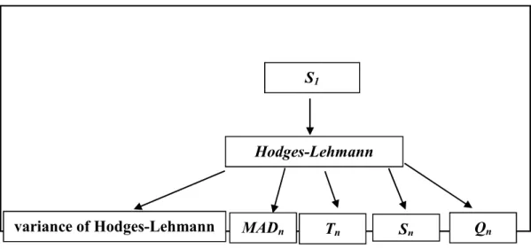
3.2 Procedure Employed……….38
3.2.1 S1 using Hodges-Lehmann with its Variance………...39
3.2.2 S1 using Hodges-Lehmann with MADn………39
3.2.3 S1 using Hodges-Lehmann with Tn………..40
3.2.4 S1 using Hodges-Lehmann with Sn………..40
3.2.5 S1 using Hodges-Lehmann with Qn……….40
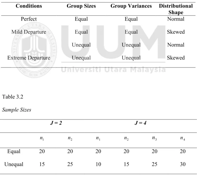
3.3 Variables Manipulated………..41
3.3.1 Number of Groups………...41
3.3.2 Balanced and Unbalanced Sample Sizes……….41
3.3.3 Types of Distributions……….42 3.3.4 Variance Heterogeneity………...43 3.3.5 Nature of Pairings………....44 3.4 Design Specification……….44 3.5 Data Generation………46 3.6 Bootstrap Method……….48
CHAPTER FOUR RESULTS OF THE ANALYSIS………50
4.1 Introduction………...50
4.2 S1 Procedures………51
4.2.1 Type I Error for J = 2………...52
4.2.1.1 Balanced Design (J = 2)………...52
4.2.1.2 Unbalanced Design (J = 2)………..53
4.2.2 Type I Error for J = 4………...55
4.2.1.1 Balanced Design (J = 4)………...55
4.2.1.2 Unbalanced Design (J = 4)………..56
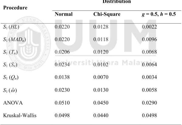
4.3 S1 Statistic versus Parametric and Nonparametric Procedures……….58
4.3.1 Type I Error J = 2 (Balanced Design)………..59
4.3.2 Type I Error J = 2 (Unbalanced Design)……….60
vii
4.3.4 Type I Error J = 4 (Unbalanced Design)……….65
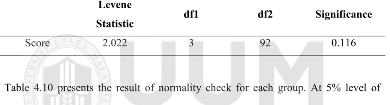
4.4 Application on Real Data………..69
CHAPTER FIVE CONCLUSION………..73
5.1 Introduction………...73
5.2 The S1 Statistic………..75
5.3 S1 Statistic versus Parametric and Nonparametric Procedures……….78
5.4 Suggestion for Future Research………84
viii
List of Tables
Table 3.1 Conditions of Departure...45
Table 3.2 Sample Sizes...45
Table 3.3 Group Variances...46
Table 3.4 Nature of Pairings...46
Table 3.5 Central Tendency Measure with respect to Distributions...48
Table 4.1 Type I Error Rates for J = 2 (Balanced Design)...52
Table 4.2 Type I Error Rates for J = 2 (Unbalanced Design)...53
Table 4.3 Type I Error Rates for J = 4 (Balanced Design)...55
Table 4.4 Type I Error Rates for J = 4 (Unbalanced Design)...56
Table 4.5 Type I Error Rates for J = 2 (Balanced Design)...59
Table 4.6 Type I Error Rates for J = 2 (Unbalanced Design)...61
Table 4.7 Type I Error Rates for J = 4 (Balanced Design)...64
Table 4.8 Type I Error Rates for J = 4 (Unbalanced Design)...66
Table 4.9 Real Data...70
Table 4.10 Test of Normality...70
Table 4.11 Test of Homogeneity of Variances...71
Table 4.12 p-value of Real Data (J = 4) ...71
Table 5.1 The Best and the Worst Procedures for Balanced Design...75
Table 5.2 The Best and the Worst Procedures for Unbalanced Design...76
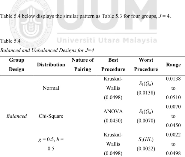
Table 5.3 Balanced and Unbalanced Designs for J = 2...78
ix
List of Figures
x
List of Abbreviations
ANOVA Analysis of Variance
HL Hodges-Lehmann Estimator
MADn Median Absolute Deviation about the Median
SAS Statistical Analysis Software
SAS/IML Statistical Analysis Software/Interactive Matrix Language SPSS Statistical Package for Social Science
1
CHAPTER ONE
INTRODUCTION
1.1 Introduction
In most research, hypothesis testing has been used as a method of decision making with the help of primary and secondary data that can be obtained from sources such as observations, experiments, journals, articles, reference books and many other sources. The researchers are required to identify the statement of null hypothesis which is usually corresponds to a situation of equality or “no difference” and it is assumed as true hypothesis until receiving an evidence that shows otherwise. Alternative hypothesis is known as the negation of null hypothesis (Sullivan, 2004). Due to the statistical nature of a test, two types of error are determined, Type I error and Type II error. Type I error occurred in the situation where by the null hypothesis is rejected when it is true. In contrast,Type II error existed when the null hypothesis is failed to reject when it is false. There is an inverse relationship between the two errors such that an increase in Type I error will decrease Type II error and vice versa. Furthermore, when Type II error increases, the statistical power of a test will decrease, causing less detection of a test effect. Thus, these two errors need to be in control. A good statistical procedure should be able to control the errors. However, working with Type I error is easier than Type II error as the earlier is usually set in advance by the researcher while the latter is harder to know as it requires estimating the distribution of the alternative hypothesis (Ramsey, 2001).
In order to achieve a good test, we need an appropriate procedure which is able to control Type I error rate and increase the power at the same time. We do not want to
2
lose power, and we do not want to inflate the Type I error rate too. There are several statistical procedures for testing the equality of location measures or locating treatment effects across groups by simultaneously controlling Type I error and improving power of the procedures in detecting the treatment effects have been studied in recent years.
Parametric procedures are widely used by researchers in many fields to test the equality of the location parameters due to precision and easy to compute. However, these procedures rely heavily on assumption of normality. For further understanding, the example of Analysis of Variance (ANOVA) and its disadvantages will be referred to with regards to violation of assumptions. ANOVA is one of the popular parametric statistical procedures which used to analyse the difference between the means for more groups in one-way independent group design. Independence of observations, normality and equality of variance (homoscedasticity) are the basic assumptions when applying this procedure. Nevertheless, violation of normality and homoscedasticity assumptions always occur in practice. These problems have degenerated the properties of Type I error and reduce the power of a test in detecting the treatment effect. When the underlying distribution has heavy tails such as symmetric heavy-tailed and skewed heavy-tail distributions, the standard error of the mean
2 n
can become seriously inflated and also reduce the power of test (Wilcox and Keselman, 2002).Thus, nonparametric statistics occurred as a field of research and several procedures turn to be very famous in applications. Nonparametric proceduresdo not rely on any
3
data belonging to any particular distribution. They are sometimes known as distribution free procedures and can be used on data such as residents’ favourite TV programmes by rating them with the scale of 1 to 10 which 1 refers to the least favour and 10 is for the most favour. Making few assumptions about the data is the basic principle of nonparametric procedures and its applicability is much wider and more robust compared to parametric procedures in most cases. Nonparametric procedures are easier to apply in most cases even though the uses of parametric procedures are justified. Nevertheless, nonparametric procedures are less powerful and a larger sample size with the same degree of confidence is required in order to reject a false hypothesis (Gibbons and Chakraborti, 2003). Under this circumstance, the use of parametric and nonparametric procedures are not advisable. To overcome the problem, robust statistical procedures are used as the alternatives.
Huber (1964) and Hampel (1974) established a complete theory of robust statistics, which basically centered on parametric models. Robust statistical procedures generally are not unduly affected by departures from the model assumptions. Besides, construction of the statistical procedures are still reliable and practically efficient in a neighbourhood of the model concerned (Ronchetti, 2006). Normality, independence and homoscedasticity are among the classical assumptions that hardly fulfilled in practice. Any violation of these assumptions will lead to biased results when tests are conducted. A definitiongiven by Hampel, Ronchetti, Rousseeuw and Stahel (1986) states that, “In a broad informal sense, robust statistics is a body of knowledge, partly formalised into “theories of robustness”, relating to deviations from idealised assumptions in statistics.”
4
The violation of normality assumption is among the most frequently discussed issue in robust statistics. This violation can reduce the power to a lower stage when the means of two or more groups are compared (Wilcox and Keselman, 2003). Refer to Md Yusof, Othman and Syed Yahaya (2010), in the study of robust statistics, Huber (1981), Staudte and Sheather (1990) and Wilcox (1997) considered robust measures of location like trimmed means or medians as the alternative solutions for the usual least squares estimator. According to Syed Yahaya, Othman and Keselman (2006), other studies had also proved that Type I error from the test of treatment effects can be well controlled through these measures of location (Othman, Keselman, Padmanabhan, Wilcox, and Fradette, 2004). A certain percentage of the smallest and largest observations are removed and averaging the remaining values is known as trimmed mean. The percentage of trimmed mean is fixed in advance to ease in analysing data. For example, 10% trimming is referred to 10% of the smallest observations and 10% of the greatest observations are trimmed. If there are 10 observations with the least value of 6 and greatest value of 35, 10% trimming is referred as removing the values of 6 and 35 follows by computing the average of the remaining observations. Yuen (1974) had found that there were some advantages on trimmed means for two groups case. Similar results on trimmed means for more than two groups case were established by Lix and Keselman (1998) and researchers were reminded that non-normality of one’s data should not automatically signal the adoption of trimmed means and robust test statistics. Researchers should take serious consideration under such circumstances about the reasons of non-normality and also to examine the method of collecting data, measurements instruments and the process
5
of generating data. Before applying trimmed mean in any research, researchers have to decide the percentage of trimming because this may cause the losing of some important information especially when the number of trimming has been decided prior to data analysis.
Besides trimmed mean, sample median, that isthe midpoint in a set of observations is also known as one of the common robust estimators especially for sufficiently heavy-tailed distributions (Wilcox, 2012). It can endure large proportion of worst observations without breaking down completely since it has been characterised by the highest breakdown point (0.5). Refer to Donoho and Huber (1983), breakdown point is roughly the smallest amount of contamination that may cause an estimator to take on arbitrarily large aberrant values. This characteristic is very helpful in understanding the robustness properties of estimators. If there are n observations and let a minority of them
n1
2n
reach infinity leaving the rest fixed, then the median stays with the majority. Therefore, the breakdown point of median in finite sample is
n1
2n
and the asymptotic breakdown point is 1 2 (0.5).Accordingto Huber (1981), for an ideal parametric model, the estimator and statistical testing of central tendency measures are always misleading by a small number of extreme values on the data sets due to their lower breakdown points. Let take sample mean as the example. Given that the observations of X1,...,Xn and the formula for mean is as below: n x x x1 2 ... n (1.1)6
If the nth observation approaches infinity, the sample mean will fall to infinity too.
This explains that the sample mean will be ruined even with one gross outlier. The breakdown point of sample mean in finite sample is 1n and the asymptotic breakdown point is zero. This means that there is only 1 n sample breakdown point of sample mean when n approaches infinity.
The following scenario is one of the examples to demonstrate the effectiveness of a robust statistics. Given that there are five measurements of a concentration, 5.59, 5.66, 5.63, 5.57 and 5.60. Normally we will calculate the sample mean for estimating its true value. The usual average of these five numbers is 5.61. Another estimator that can be used is sample median andit yields5.60. In this example, the values of mean and median are close to each other. Let us now suppose that one of the measurements is recorded wrongly such thatthe data is recorded as 5.59, 5.66, 5.63, 55.7 and 5.60. This situation often happens in research due to data entry error. There is also a possibility that the outlying observation is incorrect or it belongs to other population. Under this circumstance, the mean becomes 15.64. In contrast, the value of the medianis 5.63, which is still reasonable despite the error. The median is changed but it does not become arbitrarily bad as mean. However, median is also known as trimmed mean with 50% since 50% of the largest observations and 50% of the smallest observations are removed. This may also cause a losing of some important information.
Yi and He (2009) had done a research for longitudinal data with dropouts using median regression model. As discussed in Morgenthaler (1992), modeling the study
7
was partly inspired by longitudinal data arising from a controlled trial of HIV disease. One of the main objectives was to examine the treatment effect of Zidovudine on growing CD4+ cell counts. 892 adults were randomised to a treatment group and they were tracked longitudinally. At weeks 8, 16, 32 and 48, the measurements were collected. They tested the data using median regression model as well as mean regression model for comparison purpose. Based on the results obtained, the proposed median regression procedure performed well for a range of data with different distributions. However, mean regression approach relied on the distributional shapes. No doubt, it provided accurate results for normal distribution but it may unable to give reliable results for a data with other distributions.
1.2 Problem Statement
The letdown of parametric procedures in dealing with non-normal data and a few challenging assumptions obliged the users of statistics to opt for alternative procedures in nonparametric as well as robust procedures. However, nonparametric procedures also have their drawbacks especially in terms of losing information due to ranking process turned the users to a more reliable procedure in robust statistics.
A good robust estimator combined with good statistical procedures might be able to solve some of the typical problems encountered by the users of statistics. One of such procedures is S1 statistic which was proposed by Babu, Padmanabhan and Puri
(1999) when the distributions are skewed. This procedure comes with the purpose of measuring treatment effects across two and more than two groups by using median as the location parameter. As explained in previous section, median is the midpoint in a
8
set of observations which can endure large proportion of worst observations without breaking down completely by its highest breakdown point (0.5). Therefore, S1
statistic can deal with the original data without having to trim or transform it to attain symmetry.
Indeed, real data rarely fulfill the assumption of normality. As Reed (1998) quoted: “Nearly all real data are discrete in nature therefore the theory suggests that they cannot be normal”. According to Maxwell and Delaney (2004), the main disadvantage of data transformation is the interpretation of results may be less than clear because researchers are working in a metric other than the original variable. Besides, finding a transformation which will deal with asymmetry and variance heterogeneity simultaneously is difficult (Keselman, Wilcox, Lix, Algina and Fradette, 2007). On the other hand, trimming also may cause the losing of some important information of the data as explained in Section 1.1.
Othman et al. (2004) modified S1 statistic by replacing the standard errors of the
sample medians with asymptotic variances by referring to Hall and Sheather’s (1988) work on sample medians. For comparison purposes, the proposed procedure and the original S1 statistic were tested under the condition of non-normality and variance
heterogeneity for two groups and four groups cases. The finding showed that the proposed procedure generated slightly closer Type I error rates to nominal level of 0.05 than the original S1 statistic for four groups case. However, these error rates
were lower (deviated further away from the nominal value) than the Type I error rates produced under two groups case and were considered non robust. In addition,
9
the proposed procedures failed to show better control of Type I error compared to the original S1 statistic for two groups case.
Syed Yahaya (2005) proposed a study on testing the equality of location parameter in one-way independent group design when the distributions were skewed. S1 statistic
was selected as the procedure of the study and being modified by replacing the default scale estimator,
ˆ with four robust scale estimators, MADn, Qn, Sn and Tn.MADn is known as the famous robust scale estimator with its highest breakdown point and having the capability of maintaining the robustness of procedures. The findings proved that three out of four proposed S1 procedures using MADn, Sn and Tn as the scale estimators had good control of Type I error rates compared to the original S1 statistic under extremely skewed distributions for two and four groups
cases. However, the previous work on S1 observed that most of the conditions under
four groups case were non robust especially under the influence of extremely skewed distribution. Other than the issue of robustness, the proposed procedures generated conservative Type I error rates (below 0.025 level) in most conditions for both group designs. Thus, by using different types of location estimators, while maintaining the four robust scale estimators used in the previous study, we expect to have some significance improvement of S1 statistic in terms of controlling Type I error for
skewed distributions.
1.3 Objective(s) of the Study
The purpose of this study is to improve the original S1 statistic for testing the equality
10
distributions. In order to achieve this goal, the objectives below are required to be accomplished.
i. To modify the S1 statistic by replacing the median with the
Hodges-Lehmann.
ii. To evaluate the modified procedures with simulated data.
iii. To compare the modified procedures against some parametric and nonparametric procedures in terms of the empirical Type I error rates. iv. To compare the modified procedures against some parametric and
nonparametric procedures on real data. v. To identify the best procedures.
1.4 Significance of Study
This study will significantly contribute to the body of knowledge in statistical procedure especially experimental design which usually attached with strict assumptions such as normality and variance homogeneity to achieve reliable results. The proposed procedure gives some flexibility to the users for testing treatment effects between groups, unlike parametric procedures such as t-test and ANOVA
when the violation of assumptions exists. This flexibility should be a welcome feature for industries as they are always depend on easy to compute, fast and trustworthy statistical procedure to be employed because of the challenge of obtaining real data which is often required to fulfill the assumption of normality. Even to those users of statistical procedures who are not constantly aware of or do not pay attention on the assumptions, this type of procedure will suit them well due
11
to no additional work is needed to perform before applying it. Furthermore, it doesn’t jeopardise the results.
1.5 Organisation of the Thesis
The background of parametric, nonparametric and robust statistics are mentioned briefly in this chapter. Besides, one of the robust procedures, S1 statistic is
introduced. Further information about this procedure and recommended scale estimators will be explained in Chapter 2. In addition, some commonly used parametric and nonparametric procedures will be reviewed too. Chapter 3 will show the employment of proposed procedure and manipulation of variables. In addition, this chapter will also describe the design specification of this study. Type I error rates of each procedure will be presented and analysed in Chapter 4. Lastly, Chapter 5 will be the final chapter of the thesis that includes conclusion and suggestions for further studies.
12
CHAPTER TWO
LITERATURE REVIEW
2.1 Introduction
Parametric and nonparametric statistical procedures are available in statistical inference or hypothesis testing. Parametric procedures rely on assumptions heavily such as normality and variance homogeneity with regards of the distributional shape in the underlying population and the location parameter of the distribution. Violation of these two assumptions are often the major practical problems that is encountered by researchers when using parametric procedures especially on testing the equality of location measures for two and more than two independent groups. Conversely, nonparametric procedures do not rely on the assumptions about the distributional shape from which the sample was drawn. However, nonparametric procedures are less powerful compared to parametric procedures. Besides, in order to reject a false hypothesis, a larger sample size with the same degree of confidence is required, but practically, smaller sample size is more preferable (Gibbons and Chakraborti, 2003). Under such circumstances, the use of parametric and nonparametric procedures are not the better choice. Hence, to overcome the problem, robust statistical procedures are used as the alternatives.
Eighteenth century was the beginning of robust statistics when the first rules of outliers’ rejection were developed. In nineteenth century, these rules were formalized and implemented for estimating mean. This was followed by the development of estimators that down weight outliers. First half of the twentieth century was the period where robustness of statistical testing being considered. The need for robust
13
procedures was demonstrated by Box (1953) and Tukey (1960) (Stigler, 2010). Their research could be seen as the discovery ofrobust statistics. A few years later, Huber (1964) and Hampel (1974) established a complete theory of robust statistics, which basically centered on parametric models. As mentioned in Chapter One, robust procedures generally are not unduly affected by departures from the model assumptions. The following sections will discuss about the parametric, nonparametric and robust procedures for two and more than two groups cases that are frequently used and available in most statistical software.
2.2 Two-group Case
Suppose that
x
1i,...,
x
ni andx
1j,...,
x
njare the independent random samples from twopopulations which have continuous distribution function of
F
x
i andF
x
j respectively. Assuming the two populations’ variances are equal, there are few procedures available for testing the equality of the location parameter. Each of the commonly employed procedures from the parametric, nonparametric and robust approaches for testing the equality of central tendency measure will be discussed in the following sections in regards to their applications when violation of assumptions occur in the data. The procedures for the two group case are t-test, Mann-Whitneyand S1 Statistic.
2.2.1 t-test
The t-test is frequently used in comparing means between two groups. The validity
on drawing the accurate inferences maybe weakened if the following assumptions of
14
i. Two samples are independent.
ii. The populations follow normal probability distribution. iii. The variances of both populations are equal.
The violation of any assumption above will increase Type I error rates and also reduce the power of the procedures at the same time (Maxwell and Delaney, 2004).
When sample sizes between two groups are equal,t-test can be calculated as:
2 2 2 1 2 1 2 1 ~ ~ n s n s x x t (2.1) where 1
x= sample mean of group 1
2
x = sample mean of group 2
2 1
~
s
= estimated population variance of group 12 2
~
s
= estimated population variance of group 21
n = sample size of group 1
2
n = sample size of group 2
For unequal sample sizes, t-test can be computed as:
2 1 2 1 2 2 2 2 1 1 2 1 1 1 2 ~ 1 ~ 1 n n n n s n s n x x t (2.2)15
The degree of freedom which is used for significance testing is 2n – 2 for equation
(2.1) and n1n2 2 for equation (2.2).
Kang and Harring (2012) did a study about the impact of non-normality, effect size and sample size on two groups case for independent samples t-test. Monte Carlo
simulation with 1000 replications was used to investigate on the robustness and Type I error on two equal group sizes under non-normal distributions. The five proposed group sample sizes were n1 n2 = 8, n1 n2= 15, n1 n2= 30, n1 n2= 60 and
2 1 n
n = 120. In regards to their findings, when the distributions for both groups were non-normal and had the same distributional shape, t-test managed to maintain
its nominal Type I error rates (α = 0.05) across different sample sizes. When two distributions were non-normal and had different shapes of distribution, Type I error was slightly inflated for the sample sizes of n1 n2= 8, n1 n2= 15 and n1 n2= 30. Yet, Type I error rates were able to be upheld at its nominal level as sample size increased.
Kellermann, Bellara, Gil, Nguyen, Kim, Chen and Kromrey (2013) did a research on variance heterogeneity and non-normality using SAS Proc Test which is an easy way of testing the equality of central tendency measure for two groups. The purpose was to discover t-test’s performance under departure of normality and variance
heterogeneity. The variables that were manipulated into several conditions consisted of the total sample size, ratio of sample size, effect size for mean difference, significance level for testing the treatment effect and the alpha level for testing homogeneity. As predicted, t-test was found to perform very well in controlling Type
16
I error when the variances were equal under equal or unequal sample sizes regardless of the tenability for the assumption of normality. No doubt, t-test emerged as the best
procedure to test the difference of two independent means under this condition. However, their t-test could not adequately control Type I error when the group
variances were not equal especially for unequal sample sizes. Besides, t-test showed
a reduced in percentage on its statistical power under skewed distribution.
2.2.2 Mann-Whitney
Mann-Whitney test (Wilcoxon, 1945) is also known as Mann-Whitney U test or Wilcoxon-Mann-Whitney test. It is an alternative approach of t-test for comparing
the difference in means between two groups when the assumption of normality and variance homogeneity are not met. Its effectiveness is quite similar as t-test on
normal distribution (Sheskin, 2011). Refer to Gibbons and Chakraborti (2003), ranked data is used by Mann-Whitney for testing the central tendency measure by changing the actual numerical data to ranks in combined groups. The ranks obtained are then compared with the sums of ranks in two groups. The sampling distribution of Mann-Whitney test is approximately normal when both sample sizes are more than 10 and z test is used for statistical inferences. It is defined as:
T T T z (2.3) where
T = total of the ranks for the observations from the sample
T
= mean of the sampling distribution of T
T
17 2 ) 1 ( 1 2 1 n n n T (2.4) ) 1 ( 12 1 2 2 1 n n n n T (2.5)
Two independent samples are required and the population distributions of both samples should be equal with the exception of the central measure for the purpose of drawing valid inferences from Mann-Whitney procedure (Ott & Longnecker, 2010). Winter and Dodou (2010) studied about the comparison between Mann-Whitney and
t-test in terms of Type I and Type II error rates for five-point Likert items. In the
study, pairs of samples were drawn from fourteen diverse Likert population distributions which were considered as the representative of the possible distributions that might appear in the real Likert item data. There were ten thousand random samples selected for each of the 98 combinations of distributions. For equal sample sizes, the simulations were conducted with m = n = 10, m = n = 30 and m = n = 200.
For unequal sample sizes, m = 20, n = 5, and m = 10, n = 100, were used. The finding
showed that both procedures have same power in general except for peaked, skewed, or multimodal distributions which Mann-Whitney produced better power than t-test.
On the other hand, when m = 20, n = 5, Mann-Whitney was unable to show
robustness and good control of Type I error on one Likert item with its error rate of 0.077 at nominal significance level of 0.05. For the same Likert item and unequal sample sizes (m = 20, n = 5), t-test also couldn't control Type I error well due to its
error rate of 0.074.
Nachar (2008) used Mann-Whitney as the procedure for assessing whether two independent samples came from the same distribution. The investigation was carried
18
out on two different groups of individuals with social phobia. One group was referred to those who received behavioral therapy and another group was for the people who accepted the combined therapy of behavioral and the antibiotic with n
observations each. Since both groups showed a reduction in the number of symptoms of social phobia after each therapy, the number of these symptoms was then measured and tested under the sample sizes of 3, 4, 5, 6, 7 and 8. The finding showed that Mann-Whitney was more powerful and had better control of Type I error than t
-test when the sample size was small. However, Type I error was amplified when there was a violation of variance homogeneity.
When both populations are not normally distributed and skewed into the same direction, Mann-Whitney yielded higher power rates compared to t-test. However, if
the two groups shows different shapes of distributions, it might not be valid due to the increased in Type I error rates especially when the sample size is large (Kang and Harrings, 2012). To alleviate the problems that typically occur in t-test and
Mann-Whitney procedures, the alternative is via robust procedures.
2.2.3 S1 Statistic
One of the robust procedures that can be employed to test the equality of location parameter for two and more than two groups is S1 statistic that was proposed by
Babu, et al (1999). As explained in the previous chapter, S1 statistic uses median as
location parameter to measure the treatment effects across groups. Median is referred to as the middle value of a data set. When using this procedure, the original data can be used without going through the process of transformation or trimming. For
19
example, if a data set contains values of 3, 4, 4, 5, and 8, the mean value is 4.8. If the value of 8 is entered as 89, the sample mean will change to 21. However, under the same situation, the value of median still remains as 4 which shows that as a location measure, median is robust or not sensitive to extreme values. Hence, S1 statistic
which uses median as the location measure is recommended as an alternative robust procedure especially in dealing with skewed distributions.
To understand S1 statistic, consider the problem of comparing central tendency
measures under skewed distributions. Let
Y
ij
Y
1j,
Y
2j,...,
Y
njj
be a sample from anunknown distribution Fj and let Mj be the population median Fj: j = 1, 2,… J. For
testing H0: M1 = M2 = … = Mj versus H1: Mi ≠ Mj for at least one pair of (i, j), the S1
statistic is defined as:
J j i ij s S 1 1 (2.6) where ) ˆ ˆ ( ) ˆ ˆ ( j i j i ij M M s ; (2.7) iMˆ = the median of group i;
j
Mˆ = the median of group j;
i i i n ˆ ; j j j n ˆ ; (2.8) i
n
= number of observations for group i;j
20 2 1 1 ˆ 1
I i n j i ij i i i M X n
(2.9) 2 1 1 ˆ 1
J j n i j ij j j j M Y n (2.10)S1 in formula (2.6) is referred to the total of all possible differences between sample
medians from the J distributions divided by square root of the sum of sample
standard errors of sample medians,ˆ . Hence, the number of possible differences is similar to J(J – 1)/2 if there are J distributions.
Syed Yahaya (2005) applied S1 statistic in the study of “Robust statistical procedures
for testing the equality of central tendency parameters under skewed distributions” for two groups and more than two groups. Four robust scale estimators, MADn, Tn, Sn
and Qn were used to replace the default scale estimator of S1 statistic. Based on
Bradley’s liberal robust criterion, S1 statistic with MADn and Tn were considered
robust across all distributions for both group designs in two groups case. For four groups case, these two procedures were considered robust for normal and mildly skewed distributions under unbalanced group design. Besides, they did not show worse performance compared to the original S1 statistic for symmetric and mildly
skewed distributions. On the other hand, S1 statistic with Sn also did better than
original S1 statistic under extreme conditions. However, the procedure of S1 statistic
with Qn provided a very conservative and non-robust value for two groups and more
than two groups. In addition, all four procedures were not considered robust across all three distributional shapes for balanced group design under four groups case. The generated Type I error rates were conservative in all conditions for the same group
21
design and group case. Same issues of not robust and generating conservative Type I error rates happened on extremely skewed distribution for unbalanced group design under four groups case as well. Therefore, a suggestion for further modification on the location and scale estimators was given by the author in order to improve the performance of the S1 statistic in terms of controlling Type I error.
2.3 More than Two Groups
There are few popular parametric and nonparametric procedures readily available for testing more than two groups. One of the commonly used parametric procedure is Analysis of Variance (ANOVA) when the populations are normally distributed. If the assumption of normality is violated, nonparametric procedure such as Kruskal-Wallis is used as the alternative procedure. A robust procedure like S1 statistic also
can be applied on more than two groups case. The following sections will further explain on the aforementioned procedures.
2.3.1 Analysis of Variance (ANOVA)
Analysis of Variance (ANOVA) is known as a parametric procedure for testing the equality of two or more than two population means. There are some assumptions that have to be met. The populations are normally distributed, independent and have equal variances. However, these assumptions are hardly fulfilled in practice. Similar to t-test, the violation of assumptions give the impacts on controlling Type I error
22
The test statistic for ANOVA is based on F distribution which is a continuous
theoretical probability distribution which the F value will often fall within the range
F
0 (Sheskin, 2011). It can be computed as:
MSW MSB F (2.11) where
1 ... 2 2 2 2 2 1 1 k x x n x x n x x n MSB k k (2.12) 1n = sample size of population 1
2
n = sample size of population 2, and so on
k = number of populations
1
x = sample mean of population 1
2
x = sample mean of population 2, and so on
x = sample mean of the combined data set
k n s n s n s n MSB k k 2 22 2 2 1 1 1 1 ... 1 (2.13) 2 1s
= sample variance of population 12 2
s
= sample variance of population 2, and so onn = total number of observations of the combined data set
James (1951) and Welch (1951) recommended the estimation of the inverses of the variances of the respective sample means could be explained by weighting the terms in the sum of squares for larger sample sizes. Referred to Syed Yahaya, Md Yusof and Abdullah (2011), although ANOVA is generally known to be robust to small
23
departure from normality, the extent of this departure is unknown unless the sample size is large enough to ensure the normality. Brownie and Boss (1994) studied on the robustness of ANOVA when the number of treatments is large using agricultural screening trials which often in a blocked design with limited replication (number of blocks). The objective of the research was to identify the existence of real differences between treatments. Besides, they also wanted to determine whether the procedure could provide good performance on Type I error and have good power at the same time. Therefore, the null hypothesis, H0, of the study was “no differences between
treatments”. Based on their findings, ANOVA was considered robust only for large number of blocks under H0 although earlier statisticians had proved that both One
and Two Ways ANOVA procedures were robust to non-normality if either the number of blocks or treatments was large (Scheffe, 1959). Furthermore, the procedure couldn’t provide good power for the data with frequent extreme values.
Lix, Keselman and Keselman (1996) suggested two approaches that might be considered by the researchers when the violations of assumptions were taking place. The first approach was applying a transformation on the data and proceed with ANOVA. However, there are some limitations of transformations. The researchers may face the difficulty in interpreting the outcomes since the conclusions have to be made based on the transformed scores instead of the original observations. Besides, according to Oshima and Algina (1992), there are several transformations which can be employed on a data set that depends on the specific type and degree of assumption violation that occur. This may not always be the simple solution for researchers. Selecting an alternative statistical procedure to ANOVA which is not sensitive to the
24
assumptions such as nonparametric or robust procedure is the second approach. A nonparametric or robust procedure should be able to produce Type I error rate that is close to the nominal significance level, ,without having to concern much on the violation of assumptions. In addition, the alternative will also maintain the actual statistical power near to theoretical power (Lix, Keselman & Keselman, 1996). Further explanation of nonparametric and robust procedures will be shown in the following sections.
2.3.2 Kruskal-Wallis
Kruskal-Wallis is the well-known alternative procedure to one-way ANOVA for comparing the difference of central tendency using ranked data for at least three groups when the samples fail to meet the assumption of normality. It is a nonparametric procedure and also known as the extension of Mann-Whitney-Wilcoxon test to a design that involves more than two groups. If the result of Kruskal-Wallis is significant, it indicates that there is a significant difference across groups in the set of k groups.
All the observations in each sample that is from the different distributions are ranked from the smallest to the largest values. If there are two or more than two observations with the same value, mean of the ranks for tied values is computed. A computational formula for Kruskal-Wallis is shown below:
1
... 3
1
12 2 2 2 2 1 2 1 N n R n R n R N N H k k (2.14) where25
2 1
R = sum of the ranks squared of group 1
2 2
R = sum of the ranks squared of group 2 and so on
1
n = number of observations in group 1
2
n = number of observations in group 2
N = total number of observations
k = number of populations being compared
Khan and Rayner (2003) studied the robustness to non-normality of common tests, namely ANOVA and Kruskal-Wallis for more than two groups’ location problem. The power functions for both procedures under several conditions were generated using simulation with g (for skewness) and k (for kurtosis) distribution which was
suggested by MacGillivray and Cannon (2002). Based on the results obtained, Kruskal-Wallis performed better than ANOVA when sample sizes were large and kurtosis was high. The increase in sample size would radically improve Kruskal-Wallis’s performance. However, Kruskal-Wallis did not seem to be an appropriate procedure for small sample sizes such as n < 5 especially when normality was violated.
Kruskal-Wallis procedure must be used with caution. It is similar to F-test which is
sensitive to the occurrence of heterogeneous variances in equal and unequal sample sizes (Kruskal and Wallis, 1952). Lix. et al. (1996) did a research on a quantitative
review of alternatives to One-Way ANOVA, Kruskal-Wallis test was chosen as the alternative procedure. Similar to ANOVA, Kruskal-Wallis should be sensitive to the violation of variance homogeneity under both balanced and unbalanced designs.
26
However, the outcome of the research did not support the statement (sensitivity due to heterogeneous variances) due to the generated data. In their study, almost 90% of the balanced design data (equal group size and equal group variance) were generated whereas there were only a small percentage of unbalanced design data (unequal group size and unequal group variance) were formed. Therefore, it was difficult to create clear guidelines about the use of Kruskal-Wallis test under variance heteroscedasticity. Other than this, the procedure showed good control for non-normality data. Nevertheless, it did not perform well when the non-non-normality was found under the populations with different distributions.
The choice of estimators is crucial in controlling Type I error rate and maintaining the power of statistical procedure. Due to the violations of normality and variance homogeneity, robust estimators have received a lot of attention in the literature by wide spread list in review articles (Huber, 1972; Hogg, 1974; Dixon and Yuen, 1974). Most of the robust estimators have been established and assessed for symmetric distributions with varying degrees of heavy tailed. According to Wilcox and Keselman (2003), using robust estimators can have significantly more power when the distributions of populations are differ in skewness or have unequal variances. In addition, they show better control of Type I error. Classical parametric procedures can be considered as robust by replacing the central tendency measures with robust estimators. Hence, in order to achieve the goal of this study, Hodges-Lehmann was chosen as the robust estimate of location.
27
2.4 Hodges-Lehmann Estimator
There was a serious rejection to classical statistical procedures based on linear models or non-normality is their susceptibility to gross errors for example heavier tails than the normal distribution. This issue had overcome successfully by nonparametric procedures such as Mann-Whitney or Kruskal-Wallis. The statistical power of these procedures are more robust against gross errors that parametric procedures like t-test and ANOVA. Modifying the classical location estimators
through removal or winsorisation of outlying observations was a challenge to researchers. Hence, Hodges and Lehmann (1963) had introduced a different approach, Hodges-Lehmann estimator to these problems.
Hodges-Lehmann is a robust location estimator that derived from rank test statistics like Wilcoxon or normal scores statistics which were providing robust power successfully for the corresponding testing problems (Hodges and Lehmann, 1963). According to Boos (1982), it is a consistent and median-unbiased estimator of population mean under symmetric distribution. For skewed distribution, it estimates the “pseudo-median” which is related to population median closely. Furthermore, it is well known for having excellent robustness and efficiency properties under the usual assumption of symmetry.
Hodges-Lehmann estimator can be computed in a quick way. Let X1,..., Xn be the sample from a continuous distribution F
x F0
x
. It is given as:28 median Xi Xj ,1 i j n 2 ˆ
(2.15)The above formula is used to calculate for each group which is similar to a group mean.
Bickel (1965) studied on several robust estimates of location such as trimmed mean, winsorised mean, Hodges-Lehmann estimator and maximum likelihood estimator. By comparing to the trimmed mean, the finding suggested that Hodges-Lehmann estimator was to be preferred in any condition where the degree of contamination and shape of distribution is not known with great precision provided the computations involved are excessive. Besides, the conclusion of the study showed that all selected robust estimators, except winsorised mean behaved satisfactorily when compared to mean and Hodges-Lehmann estimator seemed to be the safest among the estimators.
Boos and Monahan (1986) proposed a procedure of incorporating prior information by replacing the likelihood in Bayes’s formula with a bootstrap estimate of the sampling density of a robust estimate of location such as trimmed mean, sample mean, sample median and Hodges-Lehmann estimator. Laplace, Uniform and Student’s t (3 df) were the three alternative error distributions that was considered in
the study with the scale of unit variance each. Based on the results obtained, all four robust estimators showed a substantial improvement for Laplace and t distributions.
Furthermore, Hodges-Lehmann estimator and trimmed mean provided the best results for t distribution by reducing the mean squared error of the posterior mean by
approximately 60%.
29
2.5 Scale Estimators
In statistics, scale estimators are used to quantify the statistical dispersion in data sets. The sample standard deviation which is thecommon measures of scale iseasily influenced by extreme value. The choice of scale measure in a test statistic is vital as this measure greatly influenced the result of the test. Othman et al. (2004) had tried
to modify S1 statistic by replacing standard error of sample median with asymptotic
variances. However, this modification was not successful as Type I error was unable to be controlled at nominal level. Syed Yahaya, Othman and Keselman (2004) then continued working on this procedure by substitutingfour robustscale estimators such as MADn, Tn, Sn and Qn in place of asymptotic variances.The substitution effectively
controlled the Type I error under normal to moderately skewed distribution but failed to do so under extremely skewed distribution. Tn, Sn and Qn were the robust scale
estimators that introduced by Rousseeuw and Croux (1993). All the four estimators were selected according to their high breakdown point and bounded influence function, which were the two important characteristics of a scale estimator.
In the next section, random sample from any distribution will be represented as
x x xn
X 1, 2,..., and medixi refers to sample median for group i.
2.5.1 MADn
Median absolute deviation about the median, MADn is a frequently used robust scale
estimator by researchers due to its best possible breakdown point of 50% which is doubled a number of interquartile range. Besides, its bounded influence function is the sharpest possible bound (Hampel, 1974). The formula is given by:
30
n
MAD b medi xi medjxj (2.16) Hampel (1974) was the first person who promoted MADn and he attributed it to
Gauss. In the formula, the constant b is needed in order to make the estimator to
remain consistent for the parameter of interest. MADn has a simple explicit formula
and only need a little time for computation. Due to the benefits of MADn, Huber
(1981) had concluded that MADn has developed as the single most useful robust scale
estimator. However, there are some disadvantages of MADn. According to
Rousseeuw and Croux (1993), it took a symmetric view on the dispersion because of the one first estimated the median and then attached the equal importance to positive and negative deviations from it. This situation did not seem to be a natural approach at asymmetric distributions which MADn was supposed to find the symmetric near
the median that consisted 50% of the data.
2.5.2 Sn
Refer to Rousseeuw and Croux (1993), Sn is one of the alternative estimators for
MADn that is used as initial or ancillary scale estimates in the similar way as MADn.
It is also able to provide high efficiency and do not slanted towards symmetric distributions. It can bedefined as:
n
S c medi
medj xi xj
(2.17) The value of c is a constant factor and its default value is 1.1926. The notation, mediis referred to the low median with the order statistic of rank
n1
2
whilemed
jis31
is quite similar to MADn but there is a slight difference between them. The operation
of
med
j was moved outside the absolute value.Sn is always uniquely defined due to its explicit formula. One of the advantages of Sn
that can overcome MADn’s drawbacks is it does not require any location estimate of
the data. Sn focuses on the typical distance between observations which is still under
asymmetric distributions instead of measuring the distance between observation and the central value. Furthermore, Sn has the greatest possible breakdown point in finite
sample by obtaining 58.23% efficiency which was better than MADn’s 36.74%
efficiency at Gaussian distributions (Rousseeuw and Croux, 1993).
2.5.3 Qn
Qn is the other alternative estimator that was suggested by Rousseeuw and Croux
(1993). This estimator is defined as:
i j
kn d x x i j
Q ; (2.18)
where d is a constant factor and
4 2 2 h n k and h
n 2 1 (2.19) Other than its simple explicit formula that is suitable for asymmetric distributions and its high breakdown point of 50%, Qn has a smooth bounded influence functionthat yields about 82% efficiency at Gaussian distributions, which is higher than Sn.
Unfortunately, Qn lost its efficiency in small samples.
32
Rousseeuw and Croux (1993) had proposed another simple explicit scale estimator with high breakdown point and suitable for asymmetric distribution, denoted as:
k j i i j h k n medx x h T
1 1 3800 . 1 (2.20)They proved that Tn has high breakdown point of 50%, a continuous influence
function with 52% efficiency which was more efficient than MADn.
According to all the estimators’ properties like breakdown point, bounded influence function and efficiency, these estimators were decided to be used as the scale estimator for S1. Syed Yahaya (2005) proposed a study to seek for alternative
procedures in testing the equality of location parameter in one-way independent group design when the distributions were skewed. In order to achieve the goal of the study, S1 statistic was modified by replacing the default scale estimator,
ˆ, withsome robust scale estimators such as MADn, Qn, Sn and Tn. According to the findings,
the modified S1 procedures were robust with the exception of Qn which generated
conservative Type I error rates (below 0.025 value). Besides, S1 statistic with Tn
performed the best among the procedures under skewed distributions.
Cui, He and Ng (2003) proposed an alternative procedure for the analysis of principal components by replacing the classical variability measure such as variance with a robust dispersion measure. For comparison purpose with classical principal components, the three chosen robust estimates of scale were trimmed standard deviation with α = 0.1, Qn and median absolute deviation, MADn. The trivariate