The European Regional Convergence Process, 1980-1995: Do Spatial Regimes and Spatial Dependence Matter?

The European Regional Convergence Process, 1980-1995:

Do Spatial Regimes and Spatial Dependence Matter?

Catherine Baumont, Cem Ertur and Julie Le Gallo

First version: March 2001

This version: July 2002

University of Burgundy,

LATEC UMR-CNRS 5118

Pôle d’Economie et de Gestion

B.P. 26611, 21066 Dijon Cedex

FRANCE

Corresponding author:

e-mail: [email protected]

web site: http://perso.wanadoo.fr/cem.ertur

∗ _{Previous versions of this paper were presented at the 40}th

European Regional Science Association Congress, Barcelona, August 29 – September 1, 2000, at the 56th Econometric Society European Meeting, Lausanne, August 25-29, 2001, at the 48th North American Meetings of the Regional Science Association International (RSAI), Charleston, South Carolina, November 15-17, 2001, at the Regional Science Seminar Series, Regional Science Applications Laboratory, University of Illinois at Urbana-Champaign, November 14, 2001, at the Spatial Econometrics Workshop, Gremaq, Toulouse 1, June 14, 2002 and at the Spatial Inequality and Development Conference, Cornell/LSE/WIDER, London, June 28-30, 2002. We would like to thank L. Anselin, R.J.G.M. Florax, R. Haining, A. Heston, P. Krugman, J. LeSage, A. Venables and Q. Xie for their valuable comments as well as all the participants/discussants at these meetings. We would also like to thank Eurostat: G. Decand and A. Behrens from the regional statistics section (division E4) as well as J. Recktenwald and I. Dennis for the help they provided on the Eurostat-Regio database. The usual disclaimer applies.

The European regional convergence process, 1980-1995:

Do spatial regimes and spatial dependence Matter?

Abstract

We show in this paper that spatial dependence and spatial heterogeneity matter in the

estimation of the β-convergence process among 138 European regions over the 1980-1995 period.

Using spatial econometrics tools, we detect both spatial dependence and spatial heterogeneity in the form of structural instability across spatial convergence clubs. The estimation of the appropriate spatial regimes spatial error model shows that the convergence process is different across regimes. We also estimate a strongly significant spatial spillover effect: the average growth rate of per capita GDP of a given region is positively affected by the average growth rate of neighboring regions.

Key words: β-convergence, spatial econometrics, spatial dependence, spatial regimes, geographic spillovers

Introduction

The convergence of European regions has been largely discussed in the macroeconomic and the regional science literature during the past decade. Two observations are often emphasized. First, the convergence rate among European regions appears to be very slow in the extensive samples considered (Barro and Sala-I-Martin, 1991, 1995 ; Sala-I-Martin, 1996a, 1996b ; Armstrong 1995a, Neven and Gouyette, 1995). Moreover, income or GDP disparities seem to be persistent despite the European economic integration process and higher growth rates of some poorer regions as highlighted in the European Commission reports (1996, 1999). These observations may indicate the existence of different groupings of regions as found in cross-country studies using international data sets (Baumol, 1986; Durlauf and Johnson, 1995; Quah, 1996a, 1997).

Second, the geographical distribution of European economic disparities is studied by López-Bazo et al. (1999) and Le Gallo and Ertur (2002) and a permanent polarization pattern between rich regions in the North and poor regions in the South is found. This evidence can be linked to several results of new economic geography theories (Krugman, 1991; Fujita et al., 1999), which show that locations of economic activities are spatially structured by some agglomerative and cumulative processes. As a result, we can say that the geographical distribution of areas characterized by high

or low economic activities is spatially dependent and tends to exhibit persistence. Moreover, the

economic surrounding of a region seems to influence the economic development perspectives for this region: a poor (respectively rich) region surrounded by poor (respectively rich) regions will stay in this state of economic development whereas a poor region surrounded by richer regions has more probability to reach a higher state of economic development. These results are highlighted for European regions by Le Gallo (2001) who analyses the transitional dynamics of per capita GDP over the 1980-1995 period by means of spatial Markov chains approach: the cluster of the poorest European regions in Southern Europe creates a great disadvantage for these regions and emphasizes a poverty trap.

All these observations lead us to analyze the convergence and growth processes among European regions over the 1980-1995 period in both a more disaggregated and comprehensive way. Indeed both economic and geographic disparities embodied in the European regional polarization pattern should be taken into account. Actually, the purpose of this paper is to show that the

introduction of spatial effects in the estimation of the β-convergence model allows doing it.

Following Anselin (1988a), spatial effects refer to both spatial autocorrelation and spatial heterogeneity. On the one hand, we emphasize the link between the detection of a positive spatial autocorrelation of regional GDPs and the regional polarization of the economies in Europe.

Moreover, we show that modeling spatial autocorrelation in the β-convergence model allows

estimating geographic spillover effects. On the other hand spatial heterogeneity means that economic behavior is not stable over space. Such a spatial heterogeneity probably characterizes patterns of economic development under the form of spatial regimes and/or groupwise heteroskedasticity: a cluster of rich regions (the core) being distinguished from a cluster of poor regions (the periphery).

From an econometric point of view, it is well known that the presence of spatial dependence and/or spatial heterogeneity leads to unreliable statistical inference based on Ordinary Least Squares (OLS) estimations. Concerning the spatial dependence issue, we use the appropriate spatial econometric tools to test for its presence and to estimate the appropriate spatial specification. Concerning the spatial heterogeneity problem, we define spatial regimes, which are interpreted as spatial convergence clubs, using Exploratory Spatial Data Analysis (ESDA) in order to capture the North-South polarization pattern observed in European regions. Taking into account both of these effects, we show two results. First, the convergence process is different across regimes. Actually there is not such a convergence process for northern regions, whereas it is weak for southern regions. Second, a significant geographic spillover effect appears in the growth process in that the average growth rate for a given region is positively influenced by the average growth rates of neighboring regions.

In a first section the convergence concepts used in this paper are presented: β-convergence, club convergence and spatial effects are defined more precisely. In the second section, the empirical methodology and the econometric results are presented. In the first step, we define convergence

clubs using ESDA. In the second step, we show that the global and a-spatial unconditional β

-convergence model is misspecified and that a spatial regime model with spatially autocorrelated errors is more appropriate. In this model, a random shock affecting a given region propagates to all the region of the sample. Two simulation experiments based on a southern region and on a northern region, illustrate this effect on the average growth rate of all the regions of our sample.

I. Convergence concepts and spatial effects

Since the rather informal contribution of Baumol (1986), and the more formal contributions of Barro and Sala-i-Martin (1991, 1992, 1995) and Mankiw, Romer and Weil (1992) among others, the controversial convergence issue has been extensively debated in the macroeconomic growth and regional science literature and heavily criticized on both theoretical and methodological grounds. The convergence hypothesis has been improved and made more precise and formal since Baumol’s

(1986) pioneering paper leading to β-convergence or σ-convergence concepts. Alternative concepts

such as club convergence (Durlauf and Johnson, 1995; Quah, 1993a, 1993b, 1996a, 1996b) or stochastic convergence (Bernard and Durlauf, 1995, 1996; Evans and Karras, 1996) have also been developed. In relation with the convergence concepts used, econometric problems, such as heterogeneity, omitted variables, model uncertainty, outliers, endogeneity and measurement errors, are often raised and alternative techniques like panel data (Islam, 1995; Caselli, Esquivel and Lefort, 1996), time series (Bernard and Durlauf, 1995, 1996; Carlino and Mills, 1993, 1996a, 1996b; Evans and Karras, 1996) and probability transition matrices (Quah, 1993a, 1996a, 1996b) are proposed. We will not attempt here to discuss this huge literature: Durlauf and Quah (1999), Islam (1998), Mankiw (1995) and Temple (1999) present outstanding surveys of this debate.

Spatial effects have received less attention in the literature although major econometric

problems are likely to be encountered if they are present in the standard β-convergence framework,

since statistical inference based on OLS will then be flawed. The first study we are aware of that takes up the issue of location and growth explicitly is De Long and Summers (1991, p. 456 and appendix 1, p. 487-490):

“Many comparative cross-country regression have assumed there is no dependence across residuals, and

that each country provides as informative and independent an observation as any other. Yet it is difficult

to believe that Belgian and Dutch economic growth would ever significantly diverge, or that substantial

productivity gaps would appear in Scandinavia. The omitted variables that are captured in the regression

residuals seem ex ante likely to take on similar values in neighboring countries. This suggests that

residuals in nearby nations will be correlated…”

However, they are disappointed not to find evidence of spatial correlation in their sample1.

Since then, the appropriate econometric treatment of these spatial effects is often neglected in the macroeconomic literature, at best it is handled by the straightforward use of regional dummies or border dummy variables (Chua, 1993; Ades and Chua, 1997; Barro and Sala-I-Martin, 1995; Easterly and Levine, 1995).

Mankiw (1995, p. 304-305) also points out that multiple regression in the standard framework treats each country as if it were an independent observation:

“For the reported standard errors to be correct, the residual for Canada must be uncorrelated with the

residual for United States. If country residuals are in fact correlated, as is plausible, then the data most

likely contain less information then the reported standard errors indicate”.

Temple (1999, p. 130-131) in his survey on the new growth evidence also draws attention to the error correlation and regional spillovers though he interprets these effects as mainly reflecting an omitted variable problem:

“Without more evidence that the disturbances are independent, the standard errors in most growth

regression should be treated with a certain degree of mistrust”.

1 _{More specifically, their result is based on regressions of normalized products of fitted residuals for all country pairs} obtained from a growth equation on different functional forms of the distance between country capitals: “We are quite surprised at the apparent absence of a significant degree of spatia l correlation in our sample…” (De Long and Summers, 1991, p. 489)

It is therefore at least surprising that these effects although acknowledged are not studied more fully in the macroeconomic literature yet appropriate statistical techniques and econometric models used for analyzing such spatial processes have been developed in the regional science literature (Anselin, 1988a; Anselin and Bera 1998; Anselin, 2001). They provide relevant tools to identify both “well defined” spatial dependence and heterogeneity forms involved in the regional growth process. Nevertheless just a few recent empirical studies apply the appropriate spatial econometric tools as Moreno and Trehan (1997), Fingleton (1999), Rey and Montouri (1999) or Maurseth (2001).

1.

ββ

-convergence models

The prediction of the neoclassical growth model (Solow, 1956) is that the growth rate of an economy will be positively related to the distance that separates it from its own steady state. This is

the concept known as conditional β-convergence. If economies have different steady states, this

concept is compatible with a persistent high degree of inequality among economies.

The hypothesis of conditional β-convergence is usually tested on the following

cross-sectional model, in matrix form:

ε φ β α + + + = S y X g_{T 0} ε ~ N(0,σ_ε2I) (1)

where g_T is the (n×1) vector of average growth rates of per capita GDP between date 0 and T; y₀

is the vector of log per capita GDP levels at date 0; X is a matrix of variables, maintaining constant

the steady state of each economy, S is the unit vector and ε is the vector of errors with the usual

properties. There is conditional β-convergence if the estimate of β is significantly negative once

X is held constant. The speed of convergence and the half-life can then be recovered using this

estimate2. This is the approach widely used in cross-country analysis, with more or less ad hoc

2

The speed of convergence is then b= −ln 1

(

)

(

)

specifications to control for the determinants of the steady state as discussed by Levine and Renelt (1992) or with specifications formally derived from structural growth models following Mankiw, Romer and Weil (1992).

If we assume that all the economies are structurally similar, characterized by the same steady state, and differ only by their initial conditions, we define the concept known as

unconditional β-convergence: all the economies converge to the same steady state. It is only in that

case that the prediction of the neoclassical growth model that poor economies grow faster than rich ones and eventually catch them up in the long run holds true.

The hypothesis of unconditional β-convergence is usually tested on the following

cross-sectional model, in matrix form:

ε β

α + +

= S y0

g_T ε ~ N(0,σ_ε2I) (2)

There is unconditionalβ–convergence when β is significantly negative. This approach is

advocated, for example, by Sala-I-Martin (1996a, 1996b) for within country cross-regional analysis

together with an increasing emphasis on the test of the σ-convergence concept, which relates to

cross-sectional dispersion. There is σ-convergence if the dispersion - measured, for example, by the

standard deviation of log per capita real GDP across a group of economies - tends to decrease over

time. These two concepts are designed to capture conceptually different phenomena: β-convergence

relates to the mobility of per capita GDP within the same distribution and σ-convergence relates to

the evolution over time of the distribution of per capita GDP. Although closely related these two

concepts are far from being identical. As is well known even unconditional β-convergence is a

necessary but not a sufficient condition for σ-convergence3.

3

However we will not use this σ-convergence concept in this paper because it is an a-spatial concept. Note that Maurseth (2001) has recently proposed a conditional σ-convergence concept, which can be interpreted as a spatialized mesure of dispersion.

2. Club convergence

However, these convergence concepts and tests have been forcefully criticized in the recent literature both on theoretical and methodological grounds and several econometric problems are often raised. More precisely, in regard with the heterogeneity problem, the concept of club convergence used for example by Durlauf and Johnson (1995) seems appealing. This concept is consistent with economic polarization, persistent poverty and clustering. In case of unconditional convergence, there is only one equilibrium level to which all economies approach. In case of conditional convergence, equilibrium differs by economy, and each economy approaches its own but unique, globally stable, steady state equilibrium. In contrast, the concept of club convergence, is based on endogenous growth models that are characterized by the possibility of multiple, locally stable, steady state equilibria as in Azariadis and Drazen (1990). Which of these different equilibria an economy will be reaching, depends on the range to which its initial conditions belong. In other words, economies converge to one another if their initial conditions are in the “basin of attraction” of the same steady state equilibrium. In such a framework, as noted by Durlauf and Johnson (1995), standard convergence tests can have some difficulties to discriminate between these multiple steady state models and the Solow model. Moreover, Bernard and Durlauf (1996) show that a linear regression applied to data generated by economies converging to multiple steady states can produce

a negative initial per capita GDP coefficient. The standard global β-convergence result appears then

to be an artifact.

Durlauf and Johnson (1995), using the Summers and Heston data set over the 1960-1985 period and the Mankiw, Romer and Weil (1992) framework, show that convergence is indeed stronger within groups of countries once they arbitrarily split the whole sample based on the initial per capita GDP level and the adult literacy rate at the beginning of the period. Moreover estimated parameter values associated to conditioning variables differ significantly across the groups. They endogenize then the splitting using the regression tree method and note the geographic homogeneity within each group but fail to find evidence of convergence among the high-output economies, that

is to say North-American and European countries. This result if furthermore qualitatively similar to that obtained by De Long (1988). They interpret the overall parameter instability as indicative of countries belonging to different regimes.

However, Galor (1996) shows that multiplicity of steady state equilibria and thus club convergence is even consistent with standard neoclassical growth models that exhibit diminishing marginal productivity of capital and constant return to scale if heterogeneity across individuals is permitted. The problem is then to distinguish evidence of club convergence from that of conditional convergence.

The standard β–convergence concept and test are also, more deeply, criticized by Friedman

(1992) and Quah (1993b) who raise the Galton’s fallacy problem. Moreover, Quah (1993a, 1996a, 1996b, 1997) argues that convergence should be studied by taking into account the shape of the entire distribution of per capita GDP and its intra-distribution dynamics over time and not by estimating the cross section correlation between growth rates and per capita GDP levels or by computing first or higher moments. Using an alternative empirical methodology based on Markov chains and probability transition matrices, Quah (1993a, 1996a, 1996b, 1997) finds evidence on the formation of convergence clubs, the international income distribution polarizing into “twin-peaks” of rich and poor countries. Quite surprisingly, Quah (1996c) does not find evidence supporting “twin-peakedness” in the European regional income distribution for a sample of 82 regions, indeed excluding southern poor Portuguese and Greek regions, over the 1980-1989 period. Yet Le Gallo (2001), using the same empirical approach, finds such evidence for an extended sample of 138 European regions over the 1980-1995 period.

In addition, Quah (1996c) raises another criticism concerning the neglected spatial dimension of the convergence process: countries or regions are actually treated as “isolated islands” in standard approaches while spatial interactions due to geographical spillovers should be taken into account. Quah (1996c, p. 954) finds that: “[…] physical location and geographical spillover matter

more than do national, macro factors” and notes that: “[…] the results highlight the importance of spatial and national spillovers in understanding regional income distribution dynamics”.

3. Spatial effects and polarization patterns

Following Anselin (1988a), spatial effects refer to both spatial dependence and spatial heterogeneity.

Spatial autocorrelation can be defined as the coincidence of value similarity with locational similarity (Anselin, 2001). Therefore, there is positive spatial autocorrelation when similar values of a random variable measured on various locations tend to cluster in space. Applied to the study of income disparities, this means that rich regions tend to be geographically clustered as well as poor regions.

Spatial heterogeneity means in turn that economic behaviors are not stable over space. In a regression model, spatial heterogeneity can be reflected by varying coefficients, i.e. structural instability, or by varying error variances across observations, i.e. heteroskedasticity. These variations follow for example specific geographical patterns such as East and West, or North and South... Such a spatial heterogeneity probably characterizes patterns of economic development under the form of spatial regimes and/or groupwise heteroskedasticity: a cluster of rich regions (the core) being distinguished from a cluster of poor regions (the periphery).

The links between spatial autocorrelation and spatial heterogeneity are quite complex. First, as pointed out by Anselin (2001), spatial heterogeneity often occurs jointly with spatial autocorrelation in applied econometric studies. Moreover, in cross-section, spatial autocorrelation and spatial heterogeneity may be observationally equivalent. For example, in polarization phenomena, a spatial cluster of extreme residuals in the center may be interpreted as heterogeneity between the center and the periphery or as spatial autocorrelation implied by a spatial stochastic process yielding clustered values in the center. Finally, spatial autocorrelation of the residuals may be implied by some spatial heterogeneity that is not correctly modeled in the regression (Brundson

et al., 1999 provide such an example). In other words, in a regression, a spatial autocorrelation of errors may simply indicate that the regression is misspecified.

Three kinds of issues arise from these complex links between spatial dependence and spatial heterogeneity.

First, we must identify spatial clusters of regional wealth upon which a spatial regimes convergence model could be based. Each spatial cluster contains all regions connected by a spatial association criterion whereas the type of spatial association differs between clusters. Then both spatial dependence and heterogeneity effects are associated in the construction of our spatial clubs.

Second, statistical inference based on OLS when heterogeneity or spatial dependence is present is not reliable. For example, if we try to estimate a model characterized by a specific form of structural instability, we cannot rely on standard tests of structural instability in presence of spatial autocorrelation and/or heteroskedasticity. It is therefore necessary to test if both effects are present. Furthermore when spatial autocorrelation and spatial heterogeneity occur jointly in a regression, the properties of White (1980) and Breusch-Pagan (1979) tests for heteroskedasticity may be flawed (Anselin and Griffith, 1988). Therefore, it is necessary to adjust structural instability and heteroskedasticity tests for spatial autocorrelation and to use appropriate econometric methods as proposed by Anselin (1988b, 1990a, 1990b).

Third, the role played by geographic spillovers in the convergence of European regions has to be considered. In a previous work, we showed that if spatial autocorrelation is detected in the

unconditional β-convergence model, then it leads to specifications integrating potential geographic

spillovers in the convergence process (Baumont, Ertur and Le Gallo, 2001). However, since spatial

heterogeneity is now integrated in the estimation of the β-convergence model, we must use

appropriate specifications and tests if we want to obtain reliable estimates of geographic spillovers on regional growth in Europe.

In the following section, we will define more precisely and apply our empirical

methodology4, which extends the approach developed by Durlauf and Johnson (1995) by explicitly

taking into account the potential spatial effects previously defined, in the framework of the standard

β- convergence process.

II. Econometric results

In the first step of our analysis, we will look for the potential of spatial autocorrelation and spatial structural instability in European regional per capita GDP in logarithms using Exploratory Spatial Data Analysis (ESDA). ESDA is a set of techniques aimed at describing and visualizing spatial distributions, at detecting patterns of global and local spatial association and at suggesting spatial regimes or other forms of spatial heterogeneity (Haining 1990; Bailey and Gatrell 1995;

Anselin 1988a, b). Moran’s I statistic is usually used to test for global spatial autocorrelation (Cliff

and Ord, 1981) while the Moran scatterplot is used to visualize patterns of local spatial association

and spatial instability (Anselin, 1996). In the second step, we will estimate an unconditional β

-convergence model by OLS and carry out various tests aiming at detecting the presence of spatial dependence and spatial heterogeneity. We will then propose the most appropriate specification in respect to these two problems.

1. Data

Data limitations remain a serious problem in the European regional context although much progress has been made recently by Eurostat. Harmonized and reliable data allowing consistent regional comparisons are scarce, in particular for the beginning of the time period under study. There is clearly a lack of appropriate or easily accessible data, to include control and environmental

variables and estimate a conditional β-convergence model, compared to the range of such variables

4

A similar empirical methodology is also used in the quite different context of criminology studies by Baller et al. (2001).

available for international studies as in Barro and Sala-I-Martin (1995) or Mankiw, Romer and Weil

(1992) (Summers and Heston data set, 1988, also called the Penn World Table)5.

We use data on per capita GDP in logarithms expressed in Ecu6. The data are extracted from

the EUROSTAT-REGIO database. This database is widely used in empirical studies on European regions, see for example López-Bazo et al. (1999), Neven and Gouyette (1995), Quah (1996), Beine and Jean-Pierre (2000) among others. Our sample includes 138 regions in 11 European countries over the 1980-1995 period: Belgium (11), Denmark (1), France (21), Germany (30), Greece (13), Luxembourg (1), Italy (20), the Netherlands (9), Portugal (5) and Spain (16) in NUTS2 and the United Kingdom (11) in NUTS1 level7 (see the data appendix for more details).

It is worth mentioning that our sample is far more consistent and encompasses much more regions than the one initially used by Barro and Sala-I-Martin (1991, 73 regions; 1995, 91 regions) and Sala-I-Martin (1996a, 73 regions; 1996b, 90 regions) mixing different sources and different regional breakdowns 8. Moreover the smaller 73 regions data set is largely confined to prosperous European regions belonging to Western Germany, France, United-Kingdom, Belgium, Denmark, Netherlands and Italy, excluding Spanish, Portuguese and Greek regions, which are indeed less prosperous. This may result in a selection bias problem raised by DeLong (1988). Armstrong (1995a, 1995b) tries to overcome these problems by expanding the original Barro and Sala-I-Martin (1991) 73 regions data set to southern less prosperous regions using a more consistent sample of 85 regions.

However, we are aware of all the shortcomings of the database we use, especially concerning the adequacy of the regional breakdown adopted, which can raise a form of the ecological fallacy problem (King, 1997; Anselin and Cho, 2000) or “modifiable areal unit problem” well known to geographers (Openshaw and Taylor, 1979, Arbia, 1989). The choice of the NUTS2

5

Levine and Renelt (1992) discuss the wide range of variables (over 50) used in various studies. 6 _{Former European Currency Unit replaced by the Euro since 1999.}

7 _{NUTS means Nomenclature of Territorial Units for Statistics used by Eurostat.}

8 _{For example, for the sample of 91 regions used by Barro and Sala-I-Martin (1995): GDP data collected by Molle} (1980) for the pre-1970 period, Eurostat data for the recent period and personal income data from Banco de Bilbao for Spanish regions for example. Button and Pentecost (1995) also report these problems.

level as our spatial scale of analysis may appear to be quite arbitrary and may have some impact on our inference results. Regions in NUTS2 level may be too large in respect to the variable of interest and the unobserved heterogeneity may create an ecological fallacy, so that it might have been more relevant to use NUTS3 level. Conversely, they may be too small so that the spatial autocorrelation detected could be an artifact that comes out from slicing homogenous zones in respect to the variable considered, so that it might have been more relevant to use NUTS1 level. Even if, ideally, the choice of the spatial scale should be based on theoretical considerations, we are constrained in empirical studies by data availability. Moreover, our preference for the NUTS2 level rather than the NUTS1 level, when data is available, is based on European regional development policy

considerations: indeed it is the level at which eligibility under Objective 1 of Structural Funds 9 is

determined since their reform in 1989 (The European regions: sixth periodic report on the socio-economic situation in the regions of the European Union, European Commission, 1999). Our empirical results are indeed conditioned by this choice and could be affected by different levels of aggregation and even by missing regions. Therefore, they must be interpreted with caution.

2. The spatial weight matrix

The spatial weight matrix is the fundamental tool used to model the spatial interdependence between regions. More precisely, each region is connected to a set of neighboring regions by means

of a purely spatial pattern introduced exogenously in this spatial weight matrix W10. The elements

ii

w on the diagonal are set to zero whereas the elements w_ij indicate the way the region i is

spatially connected to the region j. These elements are non-stochastic, non-negative and finite. In

order to normalize the outside influence upon each region, the weight matrix is standardized such

that the elements of a row sum up to one. For the variable y₀, this transformation means that the

9 _{For regions where development is lagging behind (in which per capita GDP is generally below 75% of the EU} average). More than 60% of total EU resources used to implement structural policies are assigned to Objective 1.

10 _{As pointed out by Anselin (1999b, p. 6): “Also, to avoid identification problems, the weights should truly be} exogenous to the model (Manski, 1993). In spite of their lesser theoretical appeal, this explains the popularity of geographically derived weights, since exogeneity is unambiguous”.

expression Wy₀, called the spatial lag variable, is simply the weighted average of the neighboring

observations. Various matrices can be considered: a simple binary contiguity matrix, a binary spatial weight matrix with a distance-based critical cut-off, above which spatial interactions are assumed negligible, more sophisticated generalized distance-based spatial weight matrices with or

without a critical cut-off. The notion of distance is quite general11 and different functional form

based on distance decay can be used (for example inverse distance, inverse squared distance, negative exponential etc.). The critical cut-off can be the same for all regions or can be defined to

be specific to each region leading in the latter case, for example, to k-nearest neighbors weight

matrices when the critical cut-off for each region is determined so that each region has the same number of neighbors.

It is important to stress that the weights should be exogenous to the model to avoid the identification problems raised by Manski (1993) in social sciences. This is the reason why we consider pure geographical distance, more precisely great circle distance between regional centroids, which is indeed strictly exogenous; the functional form we use is simply the inverse of squared distance which can be interpreted as reflecting a gravity function.

The general form of the distance weight matrix W k( ) we use is defined as following:

* * 2 * ( ) 0 if ( ) 1 if ( ) ( ) 0 if ( ) ij ij ij ij ij ij w k i j w k d d D k w k d D k  = =  _{= ≤}   _{= >}  and * * ( ) ( ) ( ) ij ij ij j w k =w k

∑

where d_ij is the great circle distance between centroids of regions i and j; D(1)=Q1, D(2)=Me,

3 ) 3

( Q

D = and D(4)=Max, where Q1, Me, Q3 and Max are respectively the lower quartile (321

miles), the median (592 miles), the upper quartile (933 miles) and the maximum (2093 miles) of the great circle distance distribution. This matrix is row standardized so that it is relative and not

absolute distance that matters. D k( ) is the cutoff parameter for k =1,2,3 above which interactions

11 _{Weights based on “social distance” as in Doreian (1980) or “economic distance” as in Case et al. (1993), Conley and} Tsiang (1994), Conley (1999) have also been suggested in the literature. However in that case, as noted by Anselin and Bera (1998, p.244): “… indicators for the socioeconomic weights should be chosen with great care to ensure their exogeneity, unless their endogeneity is considered explicitly in the model specification”.

are assumed negligible. For k =4, the distance matrix is full without cutoff. We therefore consider 4 different spatial weight matrices. It is important to keep in mind that all subsequent analyses are conditional upon the choice of the spatial weight matrix. Indeed the results of statistical inference

depend on spatial weights. Consequently we use k =1,2,3,4 to check for robustness of our results.

Let us finally note first that, even when using D(1)=Q1, some islands such as Sicilia, Sardegna,

and Baleares are connected to continental Europe so that we avoid rows and columns in W with

only zero values. Second, United-Kingdom is also connected to continental Europe. Third, we note that connections between southern European regions are assured so that eastern Spanish regions are connected to Baleares, which are connected to Sardegna, which is in turn connected to Italian regions, which are finally connected to western Greek regions. The block-diagonal structure of the simple contiguity matrix when ordered by country is thus avoided and the spatial connections between regions belonging to different countries are guarantied. In our opinion, these matrices have therefore more appealing features when working on a sample of European regions, which are less closely connected and less compact than US states, than the simple but less appropriate contiguity matrix.

3. Exploratory Spatial Data Analysis: detection of spatial clubs

We first test for global spatial autocorrelation in per capita GDP in logarithms using

Moran’s I statistic (Cliff and Ord, 1981), which is written in the following matrix form, for each

year t of the period 1980-1995:

0 ' ( ) ( ) . ' t t t t t z W k z n I k S z z = t = 0,...16 k =1,...,4 (4)

where z_t is the vector of the n observations for year t in deviation from the mean and W k( ) is the

spatial weight matrix. Values of I larger (resp. smaller) than the expected value

) 1 /( 1 )] ( [I k = − n−

the permutation approach with 10000 permutations (Anselin, 1995)12. It appears that, with W(1), per capita regional GDP is positively spatially autocorrelated since the statistics are significant with

0.0001

p= for every year. This result suggests that the null hypothesis of no spatial autocorrelation

is rejected and that the distribution of per capita regional GDP is by nature clustered over the whole period under study. In other words, the regions with relatively high per capita GDP (resp. low) are localized close to other regions with relatively high per capita GDP (resp. low) more often than if their localizations were purely random. A similar result holds for the average growth rate of regional per capita GDP over the whole period. Moreover these results are extremely robust in

respect to the choice of the spatial weight matrix W k( ), k =1,...,413.

Spatial instability in the form of spatial regimes is then investigated by means of a Moran

scatterplot (Anselin, 1996). Given our context of β-convergence analysis, we choose to define such

local spatial association on the logarithm of the initial level of per capita GDP. As noted by Durlauf

and Johnson (1995) the use of split variables, which are known at the beginning of the period are necessary to avoid the sample selection bias problem raised by De Long (1988).

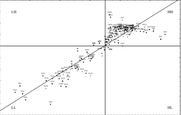
The Moran scatterplot displays the spatial lag Wy₀ against y₀, both standardized. The four

different quadrants of the scatterplot correspond to the four types of local spatial association between a region and its neighbors: (HH) a region with a high value surrounded by regions with high values, (LH) a region with a low value surrounded by regions with high values, (LL) a region with a low value surrounded by regions with low values, (HL) a region with a high value surrounded by regions with low values. Quadrants HH and LL refer to positive spatial autocorrelation indicating spatial clustering of similar values whereas quadrants LH and HL represent negative spatial autocorrelation indicating spatial clustering of dissimilar values. The Moran scatterplot may thus be used to visualize atypical localizations in respect to the global pattern, i.e. regions in quadrant LH or in the quadrant HL. A four-way split of the sample based on

12

All computations were carried out using SpaceStat 1.90 software (Anselin, 1999a). 13

In addition, the results are also robust to the use of a k-nearest neighbors spatial weight matrices, fork =10,15,20,25. Complete results are available from the authors upon request.

the two control variables, initial per capita GDP and initial spatially lagged per capita GDP, allowing for interactions between them, can therefore be based on this Moran scatterplot.

[Figure 1 about here]

Figure 1 displays this Moran scatterplot computed with W(1) for log per capita GDP in

1980. It reveals the predominance of high-high and low-low clustering types of regional per capita GDP: almost all the European regions are characterized by positive spatial association since 90 regions are of type HH and 45 regions of type LL. The Moran scatterplot confirms the clear North-South polarization of the European regions: northern regions are located in the HH quadrant while southern regions are located in the LL quadrant. Only three regions show a spatial association of dissimilar values: Wales, and Northern Ireland (United Kingdom) are located in the LH quadrant, which indicates poor regions, surrounded on average by rich regions, conversely Scotland is located in the HL quadrant.

This suggests some kind of spatial heterogeneity in the European regional economies, the convergence process, if it exists, could be different across regimes. We consider therefore two spatial clubs constituted by HH and LL regions, which we call North and South. Since Wales,

Scotland and Northern Ireland are deleted14, our new sample contains 135 regions, which belong to

North and South as following:

1/ North = {France, Germany, Netherlands, Belgium, Denmark, Luxembourg, United

Kingdom (excepted Wales, Scotland and Northern Ireland) and northern Italy (Piemonte, Valle d’Aosta, Liguria, Lombardia, Trentino-Alto Adige, Veneto, Friuli-Venezia Guilia, Emilia-Romagna and Toscana)}.

2/ South = {Portugal, Spain, Greece and southern Italy (Umbria, Marche, Lazio, Abruzzo,

Molise, Campania, Puglia, Basilacata, Calabria, Sicilia and Sardegna)}.

Not surprisingly, regions belonging to the South regime correspond to the Objective 1 regions and mainly belong to the “cohesion countries” defined by the European Commission.

14

The spatial clubs (LH) and (HL) containing only 2 regions and one region respectively are omitted due to the small number of observations in each and lack of degrees of freedom for the second step of our analysis.

The Moran scatterplots computed with the other spatial weight matrices W(2), W(3) and (4)

W lead to sensibly the same clubs: the only difference is the presence of Scotland in the North

regime. This highlights again the robustness of our results in regard to the choice of the spatial

weight matrix15. Moreover the observed polarization seems to be persistent over the whole period

since the composition of the clubs defined by the Moran scatterplots computed for each year remains globally unchanged.

The Moran scatterplot is illustrative of the complex interrelations between global spatial autocorrelation and spatial heterogeneity in the form of spatial regimes. Global spatial

autocorrelation is reflected by the slope of the regression line of Wy₀ against y₀, which is formally

equivalent to Moran’s I statistic for a row-standardized weight matrix. It seems to be inherent to the

layout of the spatial regimes corresponding to a clear North-South polarization pattern.

These exploratory results suggest that great care must be taken in the second step of our

analysis concerning the estimation of the standard β-convergence model due to the presence of

spatial autocorrelation and spatial heterogeneity. Standard estimation by OLS and statistical inference based on it are therefore likely to be misleading. Moreover, in respect to the simulation results presented by Anselin (1990a) on size and power of traditional tests of structural instability in presence of spatially autocorrelated errors, we are potentially in the worst case: positive global spatial autocorrelation and two regimes corresponding to closely connected or compact observations. These standard tests are also likely to be highly misleading. Concerning the methodological approach to be taken in empirical studies we will follow Anselin’s suggestion: “…it is prudent to always carry out a test for the presence of spatial error autocorrelation… If there is a strong indication of spatial autocorrelation, and particularly when it is positive and/or the regimes correspond to compact contiguous observations, the standard techniques are likely to be unreliable and a maximum-likelihood approach should be taken” (Anselin, 1990a, p. 205). We are aware that

15 _{Using k-nearest neighbors spatial weight matrices, we obtained the same North-South polarization result. The} complete results are available from the authors upon request.

this empirical approach raises the well known pretest problem invalidating the use of the usual asymptotic distribution of the tests, but the simulation results presented by Anselin (1990a) indicate that this problem may not be so harmful in this case.

Finally, the determination of the different regimes or clubs should, ideally, be endogenous as, for example Durlauf and Johnson (1995) in a non-spatial framework. However, to our knowledge, such an attempt has still not been made in a setting that also takes into account spatial

dependence16 and remains beyond the scope of this paper.

4. Estimation results

We first estimate the model of unconditional β-convergence by OLS and carry out various

tests aiming at detecting the presence of spatial dependence using the spatial weight matrices previously specified and spatial heterogeneity in the form of groupwise heteroskedasticity and/or structural instability across the spatial regimes previously defined. However, testing for one effect in presence of the other one requires some caution (Anselin and Griffith, 1988, Anselin 1990a, 1990b). We then estimate the appropriate specifications integrating these spatial effects separately. Two kinds of econometric specifications can be used to deal with the problem of spatial dependence (Anselin, 1988a; Anselin and Bera, 1998, Anselin, 2001): the spatial error model (spatial autoregressive error or SAR model) and the spatial lag model (mixed regressive, spatial

autoregressive model). The way these models are estimated and interpreted in the context of β

-convergence models is presented in detail for example in Rey and Montouri (1999) and Baumont, Ertur and Le Gallo (2001). The way we integrate spatial heterogeneity is rather standard: we simply estimate a groupwise heteroskedastic model by FGLS and a two-regimes model by OLS. However taking into account all effects jointly and estimating an appropriate econometric specification appears to be less straightforward: we overcome the problem by estimating a spatial regimes model with spatially autocorrelated errors.

16

This matter of fact is also noted by Anselin and Cho (2000, p. 11). This issue is much more complex than in the standard non-spatial framework due to the spatial weight matrix and the spatial ordering of the observations.

OLS estimation of the unconditional ββ-convergence model and tests

Let us take as a starting point the following model of unconditional β-convergence:

1980

T

g =αS +βy +ε 2

~ N(0, _εI)

ε σ (5)

where g_T is the vector of dimension n = 135 of the average per capita GDP growth rates for each

region i between 1995 and 1980, T =15, y1980 is the vector containing the observations of per

capita GDP in logarithms for all the regions in 1980, α and β are the unknown parameters to be

estimated, S is the unit vector and ε is the vector of errors with the usual properties.

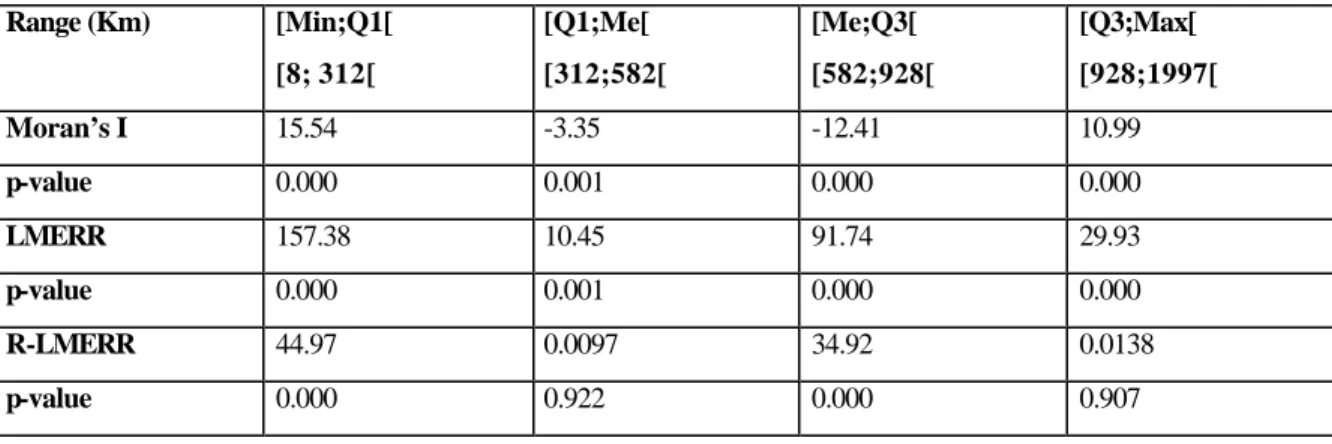
In this context, the choice of the cutoff for the distance-based spatial weight matrix W can

be based on the OLS residual correlogram with ranges defined by minimum, lower quartile, median, upper quartile and maximum great circle distances as suggested for example by Fingleton

(1999). With the sample of 135 regions we consider now, Q1, Me, Q3 and Max are modified as

following: Q1 = 312 miles, Me = 582 miles, Q3 = 928 miles and Max = 1997 miles. The

determination of the cutoff that maximizes the absolute value of significant Moran’s I test statistic

adapted to regression residuals (Cliff and Ord, 1981) or Lagrange Multiplier test statistic for spatial error autocorrelation (Anselin, 1988a, 1988b) leads to Q1: we retain a cutoff of 312 miles for the distance based weight matrix (see Table 1).

[Table 1 about here]

The results of the estimation by OLS of this model are then given in Table 2. The coefficient

associated with the initial per capita GDP is significant and negative, βˆ = −0.00797, which

confirms the hypothesis of convergence for the European regions. The speed of convergence associated with this estimation is 0.85% (the half-life is 87 years), far below 2% usually found in the convergence literature, but closer to about 1% found by Armstrong (1995a). These results indicate that the process of convergence is indeed very weak.

Evidence in favor of normality is rather week according to the Jarque-Bera test (1987) with

a p-value of 0.014. We also note that the White (1980) test clearly rejects homoskedasticity as does

the Breusch-Pagan (1979) test versus the explanatory variable y₁₉₈₀. Versus D₁, which is the

dummy variable for the northern regime, the rejection is slightly weaker with a p-value of 0.015.

Further consideration of spatial heterogeneity is therefore needed: we could think of some general form of heteroskedasticity, a more specific heteroskedasticity linked to the explanatory variable

1980

y in the regression or groupwise heteroskedasticity possibly associated to structural instability

across regimes.

Five spatial autocorrelation tests are then carried out: Moran’s I test adapted to regression

residuals (Cliff and Ord, 1981) indicates the presence of spatial dependence. To discriminate between the two forms of spatial dependence – spatial autocorrelation of errors or endogenous spatial lag - we perform the Lagrange Multiplier tests: respectively LMERR and LMLAG and their robust versions (Anselin, 1988b; Anselin et al., 1996). The two robust tests R-LMLAG and R-LMERR have a good power against their specific alternative. The decision rule suggested by Anselin and Florax (1995) can then be used to decide which specification is the more appropriate. If LMLAG is more significant than LMERR and R-LMLAG is significant but R-LMERR is not, then the appropriate model is the spatial autoregressive model. Conversely, if LMERR is more significant than LMLAG and R-LMERR is significant but R-LMLAG is not, then the appropriate specification is the spatial error model. Applying this decision rule, these tests indicate the presence of spatial error autocorrelation rather than a spatial lag variable: the spatial error model appears to be the appropriate specification. The LM test of the joint null hypothesis of absence of heteroskedasticity and residual spatial autocorrelation is highly significant whatever the form of the heteroskedasticity assumed (Anselin, 1988a, 1988b).

In addition to the apparent non-normality of the residuals, we are faced with two interconnected problems, which we have to deal with: spatial heterogeneity and spatial autocorrelation. A direct implication of these results is that the OLS estimator is inefficient and that

all the statistical inference based on it is unreliable. In addition, as pointed out earlier, we must keep in mind that in presence of heteroskedasticity, results of the spatial autocorrelation tests may be misleading and conversely results of the heteroskedasticity tests may also be misleading in presence of spatial autocorrelation (Anselin 1988a; Anselin and Griffith, 1988; Anselin 1990a,b). Therefore they must be interpreted with caution. More precisely, although the tests indicate heteroskedasticity this may not be a problem because it can be due to the presence of spatial dependence (McMillen, 1992).

The unconditional β-convergence model is strongly misspecified due to the spatial

autocorrelation and heteroskedasticity of the errors. Actually, each region cannot be considered as independent of the others. The model must be modified to integrate this spatial dependence explicitly and to take into account spatial heterogeneity. Moreover, these two aspects may be linked.

Spatial dependence

We first deal with the spatial dependence issue. We saw that the decision rule suggested by Anselin and Florax (1995) indicates a clear preference for the spatial error model over the spatial lag model. We then estimate the following SAR model:

1980

T

g =αS +βy +ε ε λ ε= W +u u ~ N(0,σ_u2I) (6)

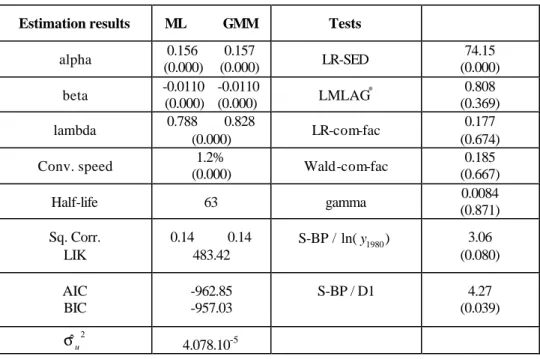
Estimation results by ML are presented in Table 3. The coefficients are all strongly

significant. From the convergence perspective, βˆ is higher than in the unconditional

β−convergence model estimated by OLS: the convergence speed is 1.2 % and the half-life reduces

to 63 years once the spatial effects are controlled for. The convergence process appears then to be a little stronger but it remains actually weak.

[Table 3 about here]

It is as well important to note that a significant positive spatial autocorrelation of the errors

restriction γ +λβ =0 cannot be rejected so the spatial error model can be rewritten as the constrained spatial Durbin model:

1980 1980

( )

T T

g =α I−λW S+β y +λWg +γWy +u (7)

with γ = −λβ , but this coefficient is not significant. From the convergence perspective, this

expression can be interpreted as a minimal conditional β-convergence model integrating two

spatial environment variables (Baumont, Ertur and Le Gallo, 2001). This reformulation has also an

interesting interpretation from an economic perspective: the average growth rate of a region i is

positively influenced by the average growth rate of neighboring regions, through the endogenous

spatial lag variable Wg_T. However, it doesn’t seem to be influenced by the initial per capita GDP of

neighboring regions, through the exogenous spatial lag variable Wy1980. This spillover effect

indicates that the spatial association patterns are not neutral for the economic performances of European regions. The more a region is surrounded by dynamic regions with high growth rates, the higher will be its growth rate. In other words, the geographical environment has an influence on growth processes.

The LMLAG* test does not reject the null hypothesis of the absence of an additional

autoregressive lag variable in the spatial error model. According to information criteria this model seems to perform better than the preceding one (Akaike, 1974; Schwarz, 1978). Moreover

estimation of this model by GMM as suggested by Kelejian and Prucha (1999)17 leads to almost the

same results on the parameters of interest. However this estimation method does not provide additional inference for the spatial autoregressive parameter, which is considered as a nuisance parameter.

The spatially adjusted Breusch-Pagan test (Anselin, 1988a, 1988b) is no more significant

( p-value of 0.08), indicating absence of heteroskedasticity versus y₁₉₈₀. If this test was the only one

carried out to detect heteroskedasticity in the spatial error model, we could say that

17

Avoiding the normality hypothesis of the error term and the problems linked to the accurate computation of the eigenvalues of W required by the ML estimator.

heteroskedasticity found in the previous model is not a problem and was due to the presence of spatial dependence. However, the spatially adjusted Breusch-Pagan test remains significant versus

1

D (p-value of 0.04). We can deduce from these results that only a part of the heteroskedasticity

found in the previous model is due to the spatial autocorrelation of the error term and that groupwise heteroskedasticity remains a problem that must be taken into account.

Spatial heterogeneity: groupwise heteroskedasticity and/or structural instability

Let us turn now to the spatial heterogeneity issue, which can be considered from two points of view. The first one relates to the heteroskedasticity problem in the form of groupwise heteroskedasticity across the regimes previously defined. The second one relates to the structural instability problem across the two regimes and furthermore may be associated to groupwise heteroskedasticity.

We estimate the following model to take account of groupwise heteroskedasticity:

1980 T g =αS +βy +ε 2 ,1 90 2 ,2 45 0 ~ 0, 0 I N I ε ε σ ε σ  _{ }  _{ }  _{ }   (8)

Estimation results by FGLS are displayed in Table 4. The coefficients are all strongly significant. ˆ

β is smaller than in all the preceding models leading to a convergence speed of 0.71 % . The

half-life raises to 102 years indicating a very weak convergence process. The difference between

regimes’ variances doesn’t seem to be significant (p-value of 0.052) as assessed by the Wald test.

However, this result should be interpreted with caution due to the presence of spatial dependence detected by the LMERR and LMLAG tests with a slight preference for spatially autocorrelated errors. Taking into account groupwise heteroskedasticity doesn’t seem to eliminate the spatial dependence and globally leads to unreliable results.

[Table 4 about here]

Let us consider more closely the possibility of structural instability. We estimate a spatial

1 1 2 2 1 1 1980 2 2 1980

T

g =αD +α D +β D y +β D y +ε ε ~ N(0,σ_ε2I) (9)

where D₁ and D₂ are dummy variables qualifying the two spatial regimes previously defined. More

precisely, D_1,i equals 1 if region i belongs to the North and 0 if region i belongs to the South; D_2,i

equals 0 if region i belongs to the North and 1 if region i belongs to the South. This model can also

be formulated in matrix form as following:

1 ,1 1 1980,1 1 1 ,2 2 1980,2 2 2 2 0 0 0 0 T T g S y Z X g S y α β ε δ ε α ε β       ₌ _{ +}  _{⇒ = +}    _{   }     _{  }     (10)

with ε'= ε₁' ε₂'_ and ε ~ N(0,σ_ε2I), the subscribe 1 standing for the north regime and the

subscribe 2 for the south regime.

This type of specification takes into account the fact that the convergence process, if it exists, could be different across regimes. Actually this approach can be interpreted as a spatial convergence clubs approach, where the clubs are identified using a spatial criterion with the Moran scatterplot as described above. Our approach extends the empirical methodology elaborated by Durlauf and Johnson (1995) to take into account explicitly the spatial dimension of data.

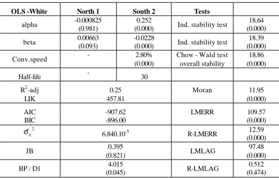
The estimation results by OLS are displayed in Table 5. We see that βˆ1 does not have the

expected sign and is not significant for the North. However, βˆ₂ has the expected sign and is

significant for southern regions leading to a convergence speed of 2.8% and a half-life of 30 years. The convergence process for southern regions seems to be stronger than the one in the initial

model18. This result is consistent with those obtained by Durlauf and Johnson (1995) The Chow test

of overall stability strongly rejects the joint null hypothesis. The individual coefficient stability tests reject the corresponding null hypotheses. The convergence process seems therefore to be quite different across regimes.

18

This result is similar to that obtained by Beine and Jean-Pierre (2000) using a sample of 62 NUTS1 regions over the 1980-1995 period with an endogenous determination of convergence clubs in an a-spatial framework.

[Table 5 about here]

It is worth mentioning that the Jarque-Bera test (1987) doesn’t reject normality (p-value of

0.82) in clear contrast to the result on the initial model: the reliability of all subsequent testing procedures and the use of Maximum Likelihood estimation method are then strengthened.

Concerning the Breusch-Pagan test versus D₁, we note that the rejection of groupwise

heteroskedasticity is weaker than in the initial model with a p-value of 0.045. The diagnostic tests

for spatial dependence still indicate a preference for spatially autocorrelated errors as in the preceding model. However all these tests should be interpreted cautiously due to the potential presence of spatially autocorrelated errors and of groupwise heteroskedasticity.

Spatial dependence and spatial heterogeneity

To take into account spatial error autocorrelation in conjunction with structural instability, we estimate the following spatial regimes model, in which we assume that the same spatial autoregressive process affects all the errors:

1 1 2 2 1 1 1980 2 2 1980

T

g =αD +α D +β D y +β D y +ε (11)

with ε λ ε= W +u and 2

~ N(0, _u )

u σ I . Or equivalently in matrix form:

1 ,1 1 1980,1 1 1 ,2 2 1980,2 2 2 2 0 0 0 0 T T g S y Z X g S y α β ε δ ε α ε β       ₌ _{ +}  _{⇒ = +}    _{   }     _{  }     (12) with ' ' 1 2 ' ε _{= }ε ε _; ε λ ε= W +u and 2 ~ N(0, _u ) u σ I .

The subscribe 1 stands for the north regime and the subscribe 2 for the south regime. This specification allows the convergence process to be different across regimes and in the same time deals with spatially autocorrelated errors previously detected. However, spatial effects are assumed to be identical in northern regions and southern regions but all the regions are still interacting

separately the two regressions allowing for different spatial effects possibly based on different spatial weight matrices across regimes. This would imply that northern and southern regions do not interact spatially and are independent. In addition, there is no obvious reason to consider different spatial weight matrices across regimes. Since the weight matrix contains the pure distance based spatial pattern, which is completely exogenous, this assumption would appear to be even more unlikely.

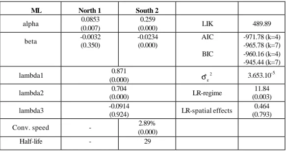
The estimation results by ML are presented in Table 6. First we note that βˆ1 and βˆ2 now

have both the expected sign but βˆ₁ is still not significant for the North. For southern regions, βˆ₂ is

strongly significant and negative. The convergence speed and the half-life are slightly improved, compared to the preceding OLS model, once the spatial effects are controlled for (respectively 2.94% and 29 years). The spatially adjusted Chow test (Anselin, 1988a, 1990a) strongly rejects the joint null hypothesis of structural stability and the individual coefficient stability tests reject the corresponding null hypotheses. These results clearly indicate that the convergence process differs across regimes. Furthermore, if there is a convergence process among European regions, it mainly concerns the southern regions and does not concern the northern regions.

[Table 6 about here]

The second aspect of these results we want to stress in this paper refers to spatial spillover effects. We first note that a significant positive spatial autocorrelation is found under this

assumption ( ˆλ=0,788). Recall that the spatial error model can also be expressed as the constrained

spatial Durbin model, which can be formulated here as:

1 1 2 2 1 1 1980 2 2 1980 1 1 1980 2 2 1980 ( ) ( ) T T g I W D I W D D y D y Wg WD y WD y u α λ α λ β β λ γ γ = − + − + + + + + + (13)

with u ~ N(0,σ_u2I) and the two nonlinear restrictions: γ₁ = −λβ₁ and γ₂ = −λβ₂. The LR and Wald

common factor tests (Burridge, 1981) indicate that these restrictions cannot be rejected. Nevertheless these two coefficients do not seem to be significant. We saw previously that this reformulation of the spatial error model has an interesting interpretation from the spatial spillover

perspective. It appears therefore that, whatever the regime, the average growth rate of a region i is positively influenced by the average growth rates of neighboring regions, through the endogenous

spatial lag variable Wg_T. However, it doesn’t seem to be influenced by the initial per capita GDP of

neighboring regions, through the exogenous spatial lag variable Wy₁₉₈₀.

The LMLAG* test does not reject the null hypothesis of the absence of an additional

autoregressive lag variable in the spatial error model. The spatially adjusted Breusch-Pagan

heteroskedasticity test versus D1 is not significant (p-value of 0.065) indicating that there is no need

to further allow for groupwise heteroskedasticity in the model. According to information criteria (Akaike, 1974; Schwarz, 1978) this model seems to perform better than all the preceding ones. Moreover estimation of this model by GMM (Kelejian and Prucha, 1999) leads to almost the same results on the parameters of interest.

Finally, the spatial regimes spatial error specification has an interesting property concerning the diffusion of a random shock. Indeed, model (11) can be rewritten as following:

1 1 1 2 2 1 1 1980 2 2 1980 ( )

T

g =αD +α D +β D y +β D y + −I λW −u (14)

Concerning the error process, this expression means that a random shock in a specific region does not only affect the average growth rate of this region, but also has an impact on the average

growth rates of all other regions through the inverse spatial transformation 1

(I−λW)− .

We present some simulation results to illustrate this property with a random shock, set equal to two times the residual standard-error of the estimated spatial regimes spatial error model, affecting Ile de France belonging to the North regime (Figure 2) and Madrid belonging to the South regime (Figure 3). This shock has the largest relative impact on Ile de France (resp. Madrid), where the estimated mean growth rate is 21.22% (resp. 20.90%) higher than the estimated average growth rate without the shock. Nevertheless, in both cases, we observe a clear spatial diffusion pattern of this shock to all other regions of the sample. The magnitude of the impact of this shock is between 1.57% and 3.74% for the regions neighboring Ile de France and gradually decreases when we move to peripheral regions (Figure 2). For Madrid, the magnitude of the impact of this shock is between

3.76% and 8.53% for the regions neighboring Madrid. As Madrid is not centrally located in Europe, the magnitude of the shock strongly decreases when we move to northern peripheral regions (Figure 3). The impact of the shock appears stronger in the South regime than in the North regime due to non-significance of the convergence parameter in the North. Therefore the spatially autocorrelated errors specification underlines that the geographical diffusion of shocks are at least as important as the dynamic diffusion of these shocks in the analysis of convergence processes.

[Figure 2 and 3 about here]

Differentiated spatial effects

Finally, we investigate the potential for differentiated spatial effects in modeling club

convergence, i.e. a different λcoefficient for each regime and a North-South interaction coefficient,

applying the methodology proposed by Rietveld and Wintershoven (1998) in a quite different context. In the previous model we assumed that spatial effects are identical across spatial clubs. This assumption should be tested. We also noted that running two separate regressions allowing for different spatial effects seems unsatisfactory because it implies that northern regions do not interact with southern regions.

An interesting way to overcome these problems is to consider the following specification:

1 1 2 2 1 1 1980 2 2 1980 T g =αD +α D +β D y +β D y +ε

(

)

where we take into account jointly structural instability and differentiated spatial effects within and

between spatial clubs. The spatial weight matrix W is now split in three part: W₁ includes only the

spatial interconnections between regions belonging to the North regime, W₂ includes only the

spatial interconnections between regions belonging to the South regime and W₃ includes only the

spatial interconnections between regions belonging to the North regime and regions belonging to the South regime. These matrices can be filled using two different approaches. The first one is