Q
ED
Queen’s Economics Department Working Paper No. 951
Bootstrap Tests: How Many Bootstraps?
Russell Davidson
GREQAM, Queen’s University
James G. MacKinnon
Queen’s University
Department of Economics
Queen’s University
94 University Avenue
Kingston, Ontario, Canada
K7L 3N6
Bootstrap Tests: How Many Bootstraps?
by
Russell Davidson
GREQAM
Centre de la Vieille Charit´e 2 rue de la Charit´e 13002 Marseille, France
Department of Economics Queen’s University Kingston, Ontario, Canada
K7L 3N6 Electronic mail: [email protected]
and
James G. MacKinnon
Department of Economics Queen’s University Kingston, Ontario, Canada
K7L 3N6
Electronic mail: [email protected]
Abstract
In practice, bootstrap tests must use a finite number of bootstrap samples. This means that the outcome of the test will depend on the sequence of random numbers used to generate the bootstrap samples, and it necessarily results in some loss of power. We examine the extent of this power loss and propose a simple pretest pro-cedure for choosing the number of bootstrap samples so as to minimize experimental randomness. Simulation experiments suggest that this procedure will work very well in practice.
This research was supported, in part, by grants from the Social Sciences and Humanities Research Council of Canada. We are grateful to Joel Horowitz, Don Andrews, several referees, and numerous seminar participants for comments on earlier work.
1. Introduction
As a result of remarkable increases in the speed of digital computers, the bootstrap has become increasingly popular for performing hypothesis tests. In econometrics, the use of the bootstrap for this purpose has been advocated by Horowitz (1994), Hall and Horowitz (1996), Li and Maddala (1996), and others. Although there are many ways to use the bootstrap for hypothesis testing, in this paper we emphasize its use to compute P values. While other ways of performing bootstrap tests are fundamentally equivalent, the P value approach is the simplest to analyze.
Following the P value approach, one first computes a test statistic, say ˆτ, in the usual way, and estimates whatever parameters are needed to obtain a data generating process (DGP) that satisfies the null hypothesis. The distribution of the random variable τ of which ˆτ is a realization under this “bootstrap DGP” serves to define the theoretical or ideal bootstrap P value, p∗(ˆτ), which is just the probability that
τ > τˆ under the bootstrap DGP. Normally this probability cannot be calculated analytically, and so it is estimated by simulation, as follows. One drawsB bootstrap samples from the bootstrap DGP, each of which is used to compute a bootstrap test statistic τ∗
j in exactly the same way as the real sample was used to compute ˆτ. For
a one-tailed test with a rejection region in the upper tail, the bootstrap P value may then be estimated by the proportion of bootstrap samples that yield a statistic greater than ˆτ: (1) pˆ∗(ˆτ)≡ 1 B B X j=1 I(τj∗ >τˆ),
where I(·) is the indicator function. As B → ∞, it is clear that the estimated bootstrapP value ˆp∗(ˆτ) will tend to the ideal bootstrap P value p∗(ˆτ).
There are two types of error associated with bootstrap testing. The first may occur whenever a test statistic is not pivotal. Although most test statistics used in econometrics areasymptotically pivotal, usually with known asymptotic distribu-tions, most of them are not pivotal in finite samples. This means that the distribution of the statistic depends on unknown parameters or other unknown features of the DGP. As a consequence, bootstrap P values will generally be somewhat inaccurate, because of the differences between the bootstrap DGP and the true DGP. Neverthe-less, inferences based on the bootstrap applied to asymptotically pivotal statistics will generally be more accurate than inferences based on asymptotic theory, in the sense that the errors are of lower order in the sample size; see Beran (1988), Hall (1992), and Davidson and MacKinnon (1998b).
The second type of error, which is the subject of this note, arises because B is necessarily finite. An ideal bootstrap test rejects the null hypothesis at level α whenever p∗(ˆτ) < α. A feasible bootstrap test rejects it whenever ˆp∗(ˆτ) < α. If
drawing the bootstrap samples and computing the τ∗
j were sufficiently cheap, we
almost always led to the same outcome. In practice, however, computing the τ∗
j is
sometimes not particularly cheap. In such cases, we want B to be fairly small. There are two undesirable consequences of using a finite number of bootstrap samples. The first is simply that the outcome of a test may depend on the sequence of random numbers used to generate the bootstrap samples. The second is that, whenever B < ∞, there will be some loss of power, as discussed in Hall and Tit-terington (1989), among others. This loss of power is often small, but, as we will see in Section 2, it can be fairly large in some cases. The principal contribution of this paper, which we introduce in Section 3, is a method for choosing B, based on pretesting, designed so that, although B is fairly small on average, the feasible and ideal tests rarely lead to different outcomes. In Section 4, we assess the performance of this procedure by simulation methods. In Section 5, we examine the performance of an alternative procedure recently proposed by Andrews and Buchinsky (1998). 2. Power Loss for Feasible Bootstrap Tests
The power loss associated with using finiteBhas been investigated in the literature on Monte Carlo tests, which are similar to bootstrap tests but apply only to pivotal test statistics. When the underlying test statistic is pivotal, a bootstrap test is equivalent to a Monte Carlo test. The idea of Monte Carlo tests is generally attributed to Dwass (1957) and Barnard (1963), and early papers include Hope (1968) and Marriott (1979). A recent application of Monte Carlo tests in econometrics can be found in Dufour and Kiviet (1998). One key feature of Monte Carlo tests is that B must be chosen so that α(B+ 1) is an integer if the test is to be exact; see the Dufour and Kiviet paper for details. Therefore, forα=.05, the smallest possible value ofBfor an exact test is 19, and forα=.01, the smallest possible value is 99. Although it is not absolutely essential to choose B in this way for bootstrap tests when the underlying test statistic is nonpivotal, since they will not be exact anyway, it is certainly sensible to do so.
Using a finite value of B inevitably results in some loss of power, because the test has to allow for the randomness in the bootstrap samples. The issue of power loss in Monte Carlo tests was first investigated for a rather special case by Hope (1968). Subsequently, J¨ockel (1986) obtained some fundamental theoretical results for a fairly wide class of Monte Carlo tests, and his results are immediately applicable to bootstrap tests.
For any pivotal test statistic and any fixed DGP, we can define the “size-power” function, η(α), as the probability under that DGP that the test will reject the null when the rejection probability under the null is α. Since the statistic is pivotal, α is well defined. This function is precisely what we plot as a size-power curve using simulation results; see, for example, Davidson and MacKinnon (1998a). It is always true thatη(0) = 0 and η(1) = 1, and we need η(α)> α for 0 < α <1 for the test to be consistent. Thus, in general, we may expect the size-power function to be concave. For tests that follow standard noncentral distributions, such as the noncentralχ2 and
the noncentralF, this is indeed so. However, it is not generally so for every test and for every DGP that might have generated the data.
Let the size-power function for a bootstrap test based on B bootstrap samples be denoted by η∗(α, m), where α(B + 1) = m. When the original test statistic is
pivotal, η(α) ≡ η∗(α,∞). Under this condition, J¨ockel (1986) proves the following
two results:
(i) Ifη(α) is concave, then so is η∗(α, m).
(ii) Assuming that η(α) is concave, η∗(α, m+ 1)> η∗(α, m).
Thus, increasing the number of bootstrap samples will always increase the power of the test. Just how much it will do so depends in a fairly complicated way on the shape of the size-power function η(α). Pivotalness is not needed if we wish to compare the powers of an ideal and feasible bootstrap test. We simply have to interpret η(α) as the size-power function for the ideal bootstrap test. Provided this function is concave, J¨ockel’s two results apply. Thus we conclude that the feasible bootstrap test will be less powerful than the ideal bootstrap test whenever the size-power function for the ideal test is concave.
J¨ockel presents a lower bound on the ratio of η∗(α, m) to η(α), which suggests
that power loss can be quite substantial, especially for small rejection probabilities under the null. From expression (4.19) of Davison and Hinkley (1997), which provides a simplified version of J¨ockel’s bound,1 we find that
(2) η(α)−η∗(α, m+ 1)≤η(α) µ 1−α 2πm ¶1/2 .
Thus the maximum power loss increases with η(α), may either rise or fall with α, and is proportional to the square root of 1/(B+ 1).
It is interesting to study how tight the bound (2) is in a simple case. We accord-ingly conducted a small simulation experiment in which we generatedt statistics for the null hypothesis that γ = 0 in the model
(3) yt =γ +ut, ut ∼N(0,1), t= 1, . . . ,4.
Theset statistics were then converted toP values. For the ideal bootstrap, this was done by using the CDF of the t(3) distribution so as to obtain p∗. For the feasible
bootstrap, it was done by drawing bootstrap test statistics from thet(3) distribution and using equation (1), slightly modified to allow for the fact that this is a two-tailed test, to obtain ˆp∗. There were one million replications.
From J¨ockel’s results, we know that it is only the size-power function that affects power loss. The details of (3) (in particular, the very small sample size) were chosen solely to keep the cost of the experiments down. They affect the results only to the extent that they affect the shapes of the size-power curves. We performed experiments
forγ = 0.5,1.0, . . . ,3.0 and present results for γ = 1.0, 2.0, and 3.0, since these three cases seem to be representative of tests with low, moderate, and high power. When γ = 1.0, the test rejected 7.6% and 29.0% of the time at the .01 and .05 levels; when γ = 2.0, it rejected 30.9% and 75.7% of the time; and whenγ = 3.0, it rejected 62.0% and 96.7% of the time.
Figure 1 shows the actual power loss observed in our experiments, together with the loss implied by the bound (2), forB= 99, which is the smallest value ofB that is commonly suggested. The shape of the bounding power loss function is quite similar to the shape of the actual power loss function, but the actual power loss is always considerably smaller than the bound. The largest loss occurs for small values of α when the test is quite powerful. In the worst case, when γ = 3.0 and α = .01, this loss is substantial: The ideal bootstrap test rejects 62% of the time, and the feasible bootstrap test rejects only 50% of the time.
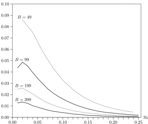
Another interesting finding is shown in Figure 2. The bound (2) implies that power loss will be proportional to (B+ 1)−1/2, but, as the figure makes clear, our
results suggest that it is actually proportional to (B + 1)−1. This suggests that,
in regular cases like the one studied in our experiments, the bound (2) becomes increasingly conservative asB becomes larger.
In order to avoid a power loss of more than, say, 1%, it is necessary to use a rather large number of bootstrap samples. If our simulation results can be relied upon, B= 399 would seem to be about the minimum for a test at the .05 level, and B= 1499 for a test at the .01 level. If there are cases in which the bound (2) is tight, then very much larger values ofB are needed.
3. ChoosingB by Pretesting
Up to this point, we have assumed thatB is chosen in advance. However, as Andrews and Buchinsky (1988) point out, if one wishes to bound the proportional error of a feasible bootstrap P value, the minimum number of bootstraps needed depends on the ideal bootstrapP value. They develop an algorithm for a data-dependent choice ofB, which we look at more closely in Section 5, designed to control the proportional error of a bootstrapP value in all cases. But, althoughP values are more informative than the yes/no result of a test at a given level α, it is often the case that specific values of α, like .05 or .01, are of special interest. In this section we propose for such cases a simple pretesting procedure for determining B endogenously.
Issues other than test power affect any such choice. When B is finite, the ran-domness of a bootstrap P value, or the result of a bootstrap test at level α, comes from two sources, the data and the simulations, these two sources being independent. We wish the outcome of a test to depend only on the first source. One way to achieve that would be to condition on the simulation randomness, but that would impose the constraint of using the same random number generator with the same seed for all bootstrap inference. Otherwise, all one can do is to seek to minimize the effect of simulation randomness. Another issue is, of course, computing time. Ceteris paribus,
it makes sense to minimize expected computing time, where the expectation is with respect to both sources of randomness. Our problem is to do so without inducing undue power loss or an unacceptably high probability of a test result in conflict with that based on the ideal bootstrap P value.
A couple of examples serve to illustrate these issues when some level α is of particular interest. If ˆτ > τ∗
j for every one of B bootstrap samples, B need not be
large for us to conclude that we should reject the null hypothesis. The probability of this event occurring by chance ifp∗(ˆτ) is equal to α is (1−α)B. ForB = 99 and
α =.05, this probability is .006. Thus, if p∗(ˆτ) is greater than or equal to .05, .006
is an upper bound on the probability that ˆτ > τ∗
j for each of 99 bootstrap samples.
Similarly, suppose that ˆp∗(ˆτ) based on B = 99 is substantially greater than .05.
According to the binomial distribution, the probability thatτ∗
j >τˆ 11 or more times
out of 99 if p∗(ˆτ) =.05 is .004. Thus, if in fact p∗(ˆτ)≤ .05, it is highly improbable
that 11 or more out of 99 bootstrap samples will produce test statistics more extreme than ˆτ.
These examples suggest a pretesting procedure in which we start with a rela-tively small value of B and then increase it, if necessary, until we are confident, at some prechosen significance level, that p∗(ˆτ) is either greater or less than α. If the
procedure stops with a small value of B, ˆp∗(ˆτ) may differ substantially from p∗(ˆτ),
but only whenp∗(ˆτ) is not close to α, thus ensuring low probability that the feasible
and ideal bootstrap tests yield different outcomes.
To implement the procedure, we must chooseβ, the level of the pretest (say .001), and two rather arbitrary parameters that can be expected to have little impact on the result of the procedure: Bmin, the initial number of bootstrap samples (say, 99),
and Bmax, the maximum number of bootstrap samples (say, 12,799). The second
parameter effectively bounds computing time, and avoids the problem that, ifp∗(ˆτ)
happens to be very close to α, then a huge number of bootstraps would be needed to determine whether it is greater or smaller than α. The procedure can be set out as follows:
1. Calculate ˆτ, set B = Bmin and B0 = Bmin, and calculate τj∗ for B = Bmin
bootstrap samples.
2. Compute ˆp∗(ˆτ) based onB bootstrap samples. Depending on whether ˆp∗(ˆτ)< α
or ˆp∗(ˆτ) > α, test either the hypothesis that p∗(ˆτ) ≥ α or the hypothesis that
p∗(ˆτ) ≤ α at level β. This may be done using the binomial distribution or,
if αB is not too small, the normal approximation to it. If ˆp∗(ˆτ) < α and the
hypothesis that p∗(ˆτ) ≥ α is rejected, or if ˆp∗(ˆτ) > α and the hypothesis that
p∗(ˆτ)≤α is rejected, stop.
3. If the algorithm gets to this step, setB = 2B0+1. IfB > B
max, stop. Otherwise,
calculateτ∗
j for a furtherB0+ 1 bootstrap samples and set B0 =B. Then return
to step 2.
The rule in step 3 is essentially arbitrary, but it is very simple, and it ensures that α(B+ 1) is an integer if α(B0+ 1) is. It is easy to see how this procedure will work.
estimate ˆp∗(ˆτ) that is relatively inaccurate, but clearly different from α. Whenp∗(ˆτ)
is reasonably close to α, the procedure will usually terminate after several rounds with an estimate ˆp∗(ˆτ) that is fairly accurate. When p∗(ˆτ) is very close to α, it will
usually terminate with B=Bmax and a very accurate estimate ˆp∗(ˆτ).
Occasionally, especially in this last case, the procedure will make a mistake, in the sense that ˆp∗(ˆτ) < α when p∗(ˆτ) > α, or vice versa. In such cases, simulation
randomness causes the result of a feasible bootstrap test at levelαto be different from the (infeasible) result of the ideal bootstrap test. If Bmax = ∞, the probability of
such conflicts between the feasible and ideal tests is bounded above byβ. In practice, with Bmax finite, the probability can be higher than β. However, the magnitude of
the difference between ˆp∗(ˆτ) and p∗(ˆτ) in the case of a conflict is bound to be very
small. In terms of the tradeoff between conflicts and computing time, it is desirable to keep β small in order to avoid conflicts when B is still small, but, for large B, the probability of conflicts can be reduced only by increasing Bmax, with a consequent
increase in expected computing time.
The procedure just described could easily be modified to handle more than one value ofα, if desired. For example, we might be interested in tests at both the .01 and .05 levels. Then step 2 would be modified so that we would stop only if ˆp∗(ˆτ)> .05
and we could reject the hypothesis that p∗(ˆτ) ≤.05, or if ˆp∗(ˆτ) < .01 and we could
reject the hypothesis that p∗(ˆτ) ≥ .01, or if .01 < pˆ∗(ˆτ) < .05 and we could reject
both the hypothesis that p∗(ˆτ)≤.01 and the hypothesis that p∗(ˆτ)≥.05.
4. The Performance of the Pretest Procedure
In order to investigate how this procedure works in practice, we conducted several simulation experiments, with two million replications each, based on the model (3), with different values of γ, Bmin, Bmax, and β. The same sequence of random
num-bers was used to generate the data for all values of these parameters. Bmin was
normally 99, and α was always .05. Because it is extremely expensive to evaluate the binomial distribution directly when B is large, we used the normal approxima-tion to the binomial whenever αB ≥ 10. Since (3) is so simple that the bootstrap distribution is known analytically, we can evaluate the ideal bootstrapP valuep∗(ˆτ)
for each replication.
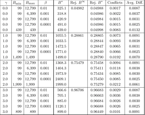
Table 1 shows results for four different values of γ. When γ = 0, so that the null hypothesis is true, B∗, the average number of bootstrap samples used by the
procedure, is quite small. As expected, reducing β and increasing Bmax both cause
B∗ to increase. As can be seen from the column headed “Conflicts”, the procedure
does indeed yield very few cases in which the feasible bootstrap test yields a different result from the ideal test. For all values of β considered, most conflicts occur when the procedure terminates with B∗ = B
max, which implies that p∗(ˆτ) is very near α
and is estimated very accurately. The last column, headed “Avg. Diff.”, shows the average absolute difference between ˆp∗(ˆτ) andp∗(ˆτ) in the few cases where there was
a conflict. It is clear that, even when the procedure yields the “wrong” answer, the investigator is not likely to be seriously misled.
The average number of bootstrap samples is higher for γ = 3 than for γ = 0, higher again for γ = 1, and higher still for γ = 2. This reflects the way in which the proportion of the p∗(ˆτ) near .05 depends on γ. When B∗ is higher, there tend to
be more cases in which the feasible and ideal bootstrap tests yield different results, because the procedure terminates more frequently withB=Bmax. It is clear that the
procedure gives rise to some power loss relative to the ideal test, but it is always very small, less than .0007 in the worst case. All of the choices of β and Bmax that were
investigated appear to yield acceptable results, and it is difficult to choose among them. We tentatively recommend settingBmax = 12,799 and choosing eitherβ =.01
or β = .001. Using the smaller value of β modestly reduces the number of conflicts and substantially reduces the average size of the conflicts that do occur, but it also seems to reduce power slightly in two cases.
The last line in the table for each value of γ shows what happens when we choose a fixed B slightly larger than the B∗ observed for the recommended values
of β and Bmax. There are far more conflicts when a fixed B is used, and they are
on average much larger, because they are based on much less accurate estimates of p∗(ˆτ). There is also substantially more power loss. Thus it appears that, holding
expected computer time constant, the pretesting procedure works very much better than using a fixed value ofB.
It is easy to understand why the pretesting procedure works well. When the null hypothesis is true, B can safely be small, because we are not concerned about power at all. Similarly, when the null is false and test power is extremely high, B does not need to be large, because power loss is not a serious issue. However, when the null is false and test power is moderately high, B needs to be large in order to avoid loss of power. The pretesting procedure tends to make B small when it can safely be small and large when it needs to be large.
5. An Alternative Procedure
In a very recent paper, Andrews and Buchinsky (1998), hereafter A-B, propose an-other method for determiningB. Their approach is based on the fact that, according to the normal approximation to the binomial distribution, if B bootstrap samples are used, then
B1/2¡pˆ∗(ˆτ)−p∗(ˆτ)¢∼N¡0, p(1−p)¢,
conditional on the randomness in the data. They wish to choose B so that the absolute value of the proportional error in ˆp∗(ˆτ) exceeds some value d, that will
generally be considerably less than 1, with probability ρ. If we write p ≡ p∗(ˆτ) for
simplicity, this implies that
(4) B = int µ χ2 1−ρ(1−p) pd2 ¶ ,
where χ2
1−ρ is the 1 −ρ quantile of the χ2(1) distribution. (A-B use somewhat
different notation, which would conflict with the notation we use in this paper.) Because (4) depends on p, which is unknown, the A-B procedure involves three steps. In the first step, it uses the (known) asymptotic distribution of τ to compute an asymptoticP value for ˆτ. This asymptoticP value is then used in (4) to calculate a preliminary number of bootstrap samples, B1, andB1 bootstrap samples are then
drawn. The bootstrap P value computed from them is then used in (4) to calculate a final number of bootstrap samples, B2. If B2 < B1, the procedure terminates with
B=B1. Otherwise, a further B2−B1 bootstrap samples are drawn.
The above description of the A-B procedure suggests that all the user need choose in advance is d and ρ. However, a little experience suggests that it is also necessary to pick Bmax, since, as is clear from (4), B1 will be extremely large when
the asymptoticP value is near zero, as willB2 when the first-stage bootstrapP value
is near zero. Moreover, it is desirable to modify the procedure slightly so that B1
andB2 both satisfy the condition thatα(B+ 1) is an integer whenα =.05, and this
implies thatB ≥19.
Unlike the procedure we have proposed, the A-B procedure is intended to give a reasonably accurate estimate of p∗ whether or not p∗ is close to α. But achieving
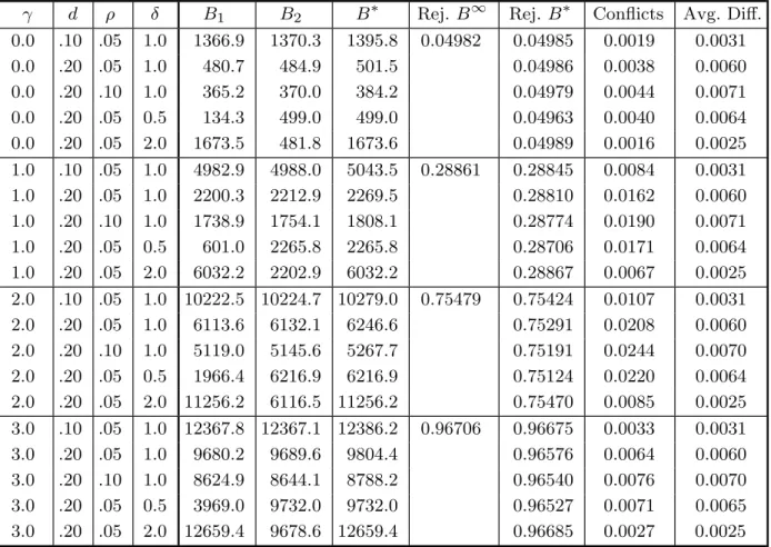
this goal entails a penalty in terms of our criteria of computing cost, power loss, and the number and magnitude of conflicts between the ideal and feasible bootstrap tests. To demonstrate these features of the A-B procedure, we performed a number of simulation experiments, comparable to those in Table 1. In these experiments, we tried several values ofd and ρand found that d=.20 and ρ=.05 seemed to provide reasonable results when γ = 0. This therefore became our baseline case. In all the experiments, we setBmin= 19 and Bmax = 12,799.
The results of our simulations are presented in Table 2. Comparing these results with those in Table 1 shows that the A-B procedure performs much less well than the pretesting procedure. Either it achieves similar performance based on far more bootstrap samples (for example, for γ = 2, compare A-B with d = .10 and ρ = .05 with any of the results in Table 1 except those withβ =.01), or else it achieves much worse performance based on a similar or larger number of bootstrap samples (for example, for γ = 1, compare A-B withd =.20 and ρ=.10 with the other procedure withBmax = 12,799 and β =.0001).
Most of our results actually show the A-B procedure in an unrealistically good light, because the asymptotic P value used to determine B1 is correct. We therefore
ran some experiments in which ˆτ was multiplied by a positive factorδ. When δ <1, the asymptotic test underrejects, and whenδ >1, it overrejects. These errors cause B1 to be chosen poorly. As can be seen from Table 2, overrejection causes the A-B
procedure to use more bootstrap samples than it should, and underrejection causes it to lose power and have more conflicts, while only slightly reducing the average number of bootstrap samples. Note that multiplying ˆτ by any positive constant has absolutely no effect on the performance of a bootstrap test with B fixed or on a bootstrap test that uses our procedure to chooseB.
6. Final Remarks
An unavoidable feature of bootstrap testing is the need to choose the number of bootstrap samples, B. In Section 2, we discussed the loss of power that can occur whenBis too small. In Section 3, we proposed a simple pretesting procedure designed to ensure that, for one or more chosen levels, feasible bootstrap tests (that is, ones with finite B) yield almost the same results as ideal bootstrap tests, while keeping B relatively small. We showed in Section 4 that this procedure works substantially better than using a fixed number of bootstrap samples. Finally, in Section 5, we showed that it also works much better than another procedure for choosing B that has recently been proposed.
References
Andrews, D. W. K. and M. Buchinsky (1998). “On the number of bootstrap repetitions for bootstrap standard errors, confidence intervals, confidence regions, and tests,” Cowles Foundation Discussion Paper No. 1141R, Yale University, revised.
Barnard, G. A. (1963). “Contribution to discussion,”Journal of the Royal Statistical Society, Series B, 25, 294.
Beran, R. (1988). “Prepivoting test statistics: a bootstrap view of asymptotic refinements,” Journal of the American Statistical Association, 83, 687–697. Davidson, R. and J. G. MacKinnon (1998a). “Graphical methods for investigating
the size and power of hypothesis tests,” The Manchester School, 66, 1–26. Davidson, R. and J. G. MacKinnon (1998b). “The size distortion of bootstrap
tests,” Queen’s University I.E.R. Discussion Paper No. 936, revised. Davison, A. C. and D. V. Hinkley (1997).Bootstrap Methods and Their
Application, Cambridge, Cambridge University Press.
Dufour, J.-M. and J. F. Kiviet (1998). “Exact inference methods for first-order autoregressive distributed lag models,” Econometrica, 66, 79–104.
Dwass, M. (1957). “Modified randomization tests for nonparametric hypotheses,”
Annals of Mathematical Statistics, 28, 181–187.
Hall, P. (1992).The Bootstrap and Edgeworth Expansion, New York, Springer-Verlag.
Hall, P. and J. L. Horowitz (1996). “Bootstrap critical values for tests based on generalized-method-of-moments estimators,” Econometrica, 64, 891–916. Hall, P. and D. M. Titterington (1989). “The effect of simulation order on level
of accuracy and power of Monte Carlo tests,” Journal of the Royal Statistical Society, Series B, 51, 459–467.
Hope, A. C. A. (1968). “A simplified Monte Carlo significance test procedure,”
Journal of the Royal Statistical Society, Series B, 30, 582–598.
Horowitz, J. L. (1994). “Bootstrap-based critical values for the information matrix test,” Journal of Econometrics, 61, 395–411.
J¨ockel, K.-H. (1986). “Finite sample properties and asymptotic efficiency of Monte Carlo tests,” Annals of Statistics, 14, 336–347.
Li, H. and G. S. Maddala (1996). “Bootstrapping time series models,” (with discussion), Econometric Reviews, 15, 115–195.
Marriott, F. H. C. (1979). “Barnard’s Monte Carlo tests: How many simulations?”
Table 1. Performance of Bootstrap Tests with B Chosen by Pretest
γ Bmin Bmax β B∗ Rej. B∞ Rej. B∗ Conflicts Avg. Diff.
0.0 99 12,799 0.01 325.1 0.04982 0.04988 0.0017 0.0087 0.0 99 6,399 0.001 318.8 0.04986 0.0022 0.0037 0.0 99 12,799 0.001 420.9 0.04984 0.0015 0.0031 0.0 99 12,799 0.0001 491.0 0.04986 0.0015 0.0025 0.0 439 439 439.0 0.04998 0.0083 0.0132 1.0 99 12,799 0.01 1055.5 0.28861 0.28865 0.0073 0.0091 1.0 99 6,399 0.001 1033.5 0.28844 0.0093 0.0038 1.0 99 12,799 0.001 1472.5 0.28847 0.0065 0.0031 1.0 99 12,799 0.0001 1771.0 0.28840 0.0066 0.0025 1.0 1,499 1,499 1499.0 0.28790 0.0192 0.0070 2.0 99 12,799 0.01 1368.3 0.75479 0.75458 0.0094 0.0091 2.0 99 6,399 0.001 1404.3 0.75411 0.0118 0.0038 2.0 99 12,799 0.001 1973.9 0.75434 0.0085 0.0030 2.0 99 12,799 0.0001 2409.1 0.75450 0.0085 0.0025 2.0 1,999 1,999 1999.0 0.75279 0.0212 0.0061 3.0 99 12,799 0.01 566.6 0.96706 0.96683 0.0029 0.0087 3.0 99 6,399 0.001 705.1 0.96663 0.0036 0.0038 3.0 99 12,799 0.001 885.0 0.96684 0.0026 0.0030 3.0 99 12,799 0.0001 1120.1 0.96688 0.0026 0.0025 3.0 899 899 899.0 0.96449 0.0101 0.0091 Notes:
B∗ is the average value of B that was finally chosen.
“Rej.B∞” is the proportion of replications for which the null hypothesis was rejected
at the .05 level according to the Student’s t distribution.
“Rej.B∗” is the proportion of replications for which the null hypothesis was rejected
at the .05 level according to the bootstrap test, based on whatever value of B was finally used.
“Conflicts” is the proportion of replications for which the ideal bootstrap test and the feasible bootstrap test yielded different inferences.
“Avg. Diff.” is the average absolute difference between the ideal and feasible boot-strap P values, for those replications which a conflict occurred.
Table 2. Performance of Bootstrap Tests withB Chosen by A-B Procedure
γ d ρ δ B1 B2 B∗ Rej. B∞ Rej. B∗ Conflicts Avg. Diff.
0.0 .10 .05 1.0 1366.9 1370.3 1395.8 0.04982 0.04985 0.0019 0.0031 0.0 .20 .05 1.0 480.7 484.9 501.5 0.04986 0.0038 0.0060 0.0 .20 .10 1.0 365.2 370.0 384.2 0.04979 0.0044 0.0071 0.0 .20 .05 0.5 134.3 499.0 499.0 0.04963 0.0040 0.0064 0.0 .20 .05 2.0 1673.5 481.8 1673.6 0.04989 0.0016 0.0025 1.0 .10 .05 1.0 4982.9 4988.0 5043.5 0.28861 0.28845 0.0084 0.0031 1.0 .20 .05 1.0 2200.3 2212.9 2269.5 0.28810 0.0162 0.0060 1.0 .20 .10 1.0 1738.9 1754.1 1808.1 0.28774 0.0190 0.0071 1.0 .20 .05 0.5 601.0 2265.8 2265.8 0.28706 0.0171 0.0064 1.0 .20 .05 2.0 6032.2 2202.9 6032.2 0.28867 0.0067 0.0025 2.0 .10 .05 1.0 10222.5 10224.7 10279.0 0.75479 0.75424 0.0107 0.0031 2.0 .20 .05 1.0 6113.6 6132.1 6246.6 0.75291 0.0208 0.0060 2.0 .20 .10 1.0 5119.0 5145.6 5267.7 0.75191 0.0244 0.0070 2.0 .20 .05 0.5 1966.4 6216.9 6216.9 0.75124 0.0220 0.0064 2.0 .20 .05 2.0 11256.2 6116.5 11256.2 0.75470 0.0085 0.0025 3.0 .10 .05 1.0 12367.8 12367.1 12386.2 0.96706 0.96675 0.0033 0.0031 3.0 .20 .05 1.0 9680.2 9689.6 9804.4 0.96576 0.0064 0.0060 3.0 .20 .10 1.0 8624.9 8644.1 8788.2 0.96540 0.0076 0.0070 3.0 .20 .05 0.5 3969.0 9732.0 9732.0 0.96527 0.0071 0.0065 3.0 .20 .05 2.0 12659.4 9678.6 12659.4 0.96685 0.0027 0.0025 Notes:
δ is a factor by which the test statistic is multiplied.
B1 is the average number of bootstraps from step 1 of the A-B procedure.
B2 is the average number of bootstraps from step 2 of the A-B procedure.
B∗ is the average number of bootstraps in total.
0.00 0.05 0.10 0.15 0.20 0.25 0.00 0.05 0.10 0.15 0.20 0.25 ... ... ...... ... ...... ... ... ... ... ... ... ... ... ... ...... ... ...... ... ... ...... ... ... ... ... ...... ...... ...... ...... ...... ... ...... ... ...... ... ...... ... ...... ... ... ...... ... ... ...... ...... ... ...... Size Power Loss γ = 3, bound γ = 3, actual γ = 2, bound γ = 2, actual γ = 1, bound γ = 1, actual
0.00 0.05 0.10 0.15 0.20 0.25 0.00 0.01 0.02 0.03 0.04 0.05 0.06 0.07 0.08 0.09 0.10 ........ ........ .... .... .... .... ........ .... ........ .... .... ... ... ...... ...... ...... ... ... ...... ...... ...... ...... ...... ...... ... ...... ... ...... ... ... ...... ... ...... ...... ... Size Power Loss B= 49 B = 99 B = 199 B = 399