5REXVWHVWLPDWLRQRIPHDQDQGGLVSHUVLRQIXQFWLRQV
LQH[WHQGHGJHQHUDOL]HGDGGLWLYHPRGHOV
&&URX[,*LMEHOVDQG,3URVGRFLPL
DEPARTMENT OF DECISION SCIENCES AND INFORMATION MANAGEMENT (KBI)
Faculty of Business and Economics
Robust estimation of mean and dispersion functions in Extended Generalized Additive Models
C. Croux1,3,4, I. Gijbels2,3 and I. Prosdocimi2,3 1 Faculty of Business and Economics
2 Department of Mathematics
3 Leuven Statistics Research Center (LStat)
Katholieke Universiteit Leuven, Belgium;
4 Tilburg University, The Netherlands.
3rd September 2010
Abstract
Generalized Linear Models are a widely used method to obtain parametric es-timates for the mean function. They have been further extended to allow the re-lationship between the mean function and the covariates to be more flexible via Generalized Additive Models. However the fixed variance structure can in many cases be too restrictive. The Extended Quasi-Likelihood (EQL) framework allows for estimation of both the mean and the dispersion/variance as functions of covari-ates. As for other maximum likelihood methods though, EQL estimates are not resistant to outliers: we need methods to obtain robust estimates for both the mean and the dispersion function. In this paper we obtain functional estimates for the mean and the dispersion that are both robust and smooth. The performance of the proposed method is illustrated via a simulation study and some real data examples.
Keywords: dispersion, generalized additive modelling, mean regression function,
quasi-likelihood, M-estimation, P-splines, robust estimation.
1
Introduction
Statistical modelling aims at describing how a phenomenon of interest changes with re-spect to some other quantities. Generally most of the modelling efforts focus on studying how the expected value of the dependent variable Y, denoted byµ, changes as a function of the covariates Xd = (X1, . . . , Xd). Generalized Linear Models (GLM McCullagh and
Nelder (1989)) are one of the most popular techniques to model the mean of different types of distributions belonging to the Exponential Family. Standard GLM though are
not always most appropriate to model the data at hand; the assumption of a linear rela-tionship between (a transformation of)µand the covariates might be too restrictive. Also, GLM estimates are maximum likelihood estimates, which can be severely influenced by the presence of outliers. For both issues possible solutions have been proposed: we can al-low the relationship between (a transformation of)µand the covariates to be of a smooth unknown shape via Generalized Additive Models (GAM Hastie and Tibshirani (1990)) and we can obtain estimates that are robust via the approach proposed for GLM’s by Cantoni and Ronchetti (2001a). Recently Alimadad and Salibian-Barrera (2009) propose a method for robust estimation of GAM.
In this paper we develop a statistical procedure to obtain smooth and robust estimates for both the mean and the dispersion function in a multivariate covariates setting. We thus allow for heteroscedasticity in the model. Estimating how the variance changes with respect to Xd can be in some cases of interest by itself, or it can be pursuit to obtain a
more appropriate fit. From the distributional assumptions made in GLM follows a fixed relationship between the shape of the variance and the mean, but the variance observed in real data often deviates from the theoretical model. Common deviations from the usual assumptions in GLM are heteroscedasticity in normal data and over- or under- dispersion in count and proportion data. The estimation of the variance can indeed be a crucial point and different approaches have been proposed to tackle this problem: see the introduction in Gijbels et al. (2010) or Hinde and Dem´etrio (1998) for a review of possible methods. In this work we use the Extended Quasi-likelihood approach (Nelder and Pregibon (1987) and McCullagh and Nelder (1989)) to obtain estimates for the dispersion function. Just as the standard Quasi-likelihood, Extended Quasi-likelihood estimators can be severely affected by outliers, and we use the techniques proposed by Cantoni and Ronchetti (2001a) to robustly estimate both the mean and the dispersion function in our setting. Moreover, the methods presented here allow these estimates to be a flexible function of the covariates. The remainder of the paper is organized as follows: in Sections 2 and 3 standard and ro-bust estimation methods within the Extended Quasi-likelihood framework are presented. In Section 4 we introduce the Generalized Additive Models framework to obtain smooth and robust estimates of the mean and the dispersion function. In Section 5 we discuss how to optimally choose the smoothing parameters for both the robust and the standard Generalized Additive Models. We show the performance of the proposed methods via a simulation study and real data examples in Sections 6 and 7 respectively.
2
Extended Quasi-likelihood
In order to write a likelihood function for a certain model, we need to make assumptions on the distribution of the process of interest. In the Quasi-likelihood framework, rather than making a full distributional assumption, one only specifies the relationship between the mean and the variance of the process of interest. Estimates are obtained by maximizing a Quasi-likelihood function, which shares key properties with a likelihood function, but can be obtained with weaker assumptions (Wedderburn (1974)). We consider
E[Y|Xd=xd] =µ(xd) and Var[Y|Xd=xd] =φV(µ(xd)),
with V(·) a known function, and write the Quasi log-likelihood function as:
Q(y, µ(xd)) =
Z µ(xd)
y
y−t φV(t)dt .
We also introduce a monotone and twice differentiable function η(·), which transforms the expected value of (Y|Xd =xd) via a link function g(·), and is modelled as a linear
combination of some generic functions of the covariates: η(xd) = g(µ(xd)) = αµ,0 +
η1(x1) +. . .+ηd(xd). Furthermore, the quasi-deviance function
d(y, µ(xd)) =−2Q(y, µ(xd)) = 2
Z y
µ(xd)
y−t
φV(t)dt , (2.1)
measures the discrepancy between the value of y and the expected value of the original distribution.
In the Quasi-likelihood setting the relationship between the variance of (Y|Xd =
xd) and the covariates is totally governed by the functional form of V(µ(xd)). This
relationship might however be too restrictive, and one might be interested in adding an extra dispersion parameter in the model which varies as a function of the covariates (Nelder and Pregibon (1987)). We thus consider
E[Y|Xd =xd] =µ(xd) and Var[Y|Xd=xd] =φγ(xd)V(µ(xd)), (2.2)
with γ(xd) an extra dispersion function. In order to model this dispersion function we
take:
E[d(Y, µ)|Xd =xd] =γ(xd) and Var[d(Y, µ)|Xd =xd] = 2γ2(xd). (2.3)
The structure used to model the dispersion is a mirror image of the mean modelling: the quasi-deviance is used as a ‘response’ variable with mean function γ(xd) and a suitable
variance function is also assumed. Note how the chosen variance structure for the disper-sion corresponds to assuming (d(Y, µ)|Xd =xd)∼γ(xd)χ21. We introduce here a second
monotone and twice differentiable function ξ(·), which transforms the expected value of (d(Y, µ)|Xd= xd) via a link function h−1(·), and is modelled as a linear combination of
some generic functions of the covariates: ξ(xd) =h−1(γ(xd)) =αγ,0+ξ1(x1)+. . .+ξd(xd).
In the usual parametric approach one takes the relationship between the link functions and the covariates Xd to be linear: η(xd) = αµ,0 +x1αµ,1 +. . .+xdαµ,d and ξ(xd) =
αγ,0+x1αγ,1+. . .+xdαγ,d with αµ= (αµ,0, αµ,1, . . . , αµ,d) and αγ = (αγ,0, αγ,1, . . . , αγ,d)
the vectors of parameters which need to be estimated.
We propose to estimate the αµ and αγ in a two-steps procedures which alternates
between the estimation of αµ and αγ as in McCullagh and Nelder (1989). For a given
i.i.d. sample (x,y) = ((xd,1, y1)T, . . . ,(xd,n, yn)T)T, we take the n ×(d + 1) regression
matrix Bµ = [1n x] where we denote with 1n = (1, . . . ,1)T the unit vector of length n.
We model η(x) = Bµαµ. The Extended Quasi-likelihood estimator of αµ is then the
solution to BTµ y−µ(x) φγV(µ(x)) dµ dη(x) =0, (2.4)
where0is the null vector,µ(x) = (µ(xd,1,αµ), . . . , µ(xd,n,αµ))T is the vector of computed
µ(·) values for each data point and V(µ(x)) is the vector of values of the V(·) function evaluated at each µ(x) point. The multiplication of the vectors within the brackets is done element-wise. In the notation we drop the dependence of µ(x) on αµ to make the
formulas more readable. By γ(x) = (γ(xd,1,αγ), . . . , γ(xd,n,αγ))T we denote the vector
of γ(·) values for each data point. While we estimate αµ we take αγ, and therefore γ,
to be fixed. Once that αµ, and consequently µ(x), is estimated by solving (2.4), we
compute the vector of deviances d = d(y,µ) = (d(y1, µ(xd,1))T, . . . , d(yn, µ(xd,n))T)T,
where µ = µ(x) = (µ(xd,1), . . . , µ(xd,n)), is now taken to be a fixed vector. Taking
Bγ = [1n x] we model ξ(x) = Bγαγ and estimate αγ by solving:
BTγ d−γ(x) 2γ2(x) dγ dξ(x) =0.
3
Robust estimation of mean and dispersion
The Extended Quasi-likelihood (EQL) estimators proposed in Section 2 can been shown to have an unbounded influence function. Outlying points, as well as bad leverage points, can have a severe effect on the performance of the estimator. To mitigate the effect of
outliers and to obtain bounded influence functions, an M-type estimation procedure is followed similar as in Cantoni and Ronchetti (2001a).
The M-estimator for αµ is obtained as the solution of the equation:
Ψs(y, µ(x)) =BTµ(sψ(y, µ(x))w(x)µ′−a(αµ)) =0, (3.1)
with µ′ = dµ
dη(x). Robustness against outlying points is obtained if Ψs(·,·) is a bounded
function. For this, we take
sψ(y, µ(xd)) =ψc y−µ(x) p φγV(µ(x)) ! 1 p φγV(µ(x)) , with ψc the Huber function defined as
ψc(x) =
(
x if |x| ≤c
c sign(x) if |x|> c . (3.2)
Further w(·) in (3.1) is a weight function which controls the effect of leverage points on the estimate.
The tuning constant c in (3.2) balances the robustness and the efficiency of the esti-mate; if w(x) =1n and c=∞ (3.1) boils down to (2.4). Cantoni and Ronchetti (2001a)
discuss procedures to choose c. Unless otherwise stated, we take c= 1.345, the standard value which ensures 95% efficiency for the normal model. Our experience shows that this value gives reasonable results for other models as well. In (3.1) the constant
a(αµ) = ¯En[sψ(y, µ(x))|Xd =xd]w(x)µ′
ensures Fisher consistency. Here we used the shorthand notation ¯En[sψ(y, µ(x))|Xd =xd]
for n−1Pn
i=1E[sψ(Y, µ(Xd))|Xd =xd,i]. This notation ¯En will also be used in the next
paragraph with a similar meaning involving a different quantity. Similarly, a robust estimate for αγ is obtained as the solution to:
Ψt(d, γ(x)) = BTγ (tψ(d, γ(x))w(x)γ′−b(αγ)) =0, (3.3)
withγ′ = dγ
dξ(x). The estimate is robust against outliers, provided that we take Ψt(d, γ(x))
to be a bounded function. As for the estimation of αµ we take
tψ(d, γ(x)) =ψc d−γ(x) √ 2γ(x) 1 √ 2γ(x), with ψc the Huber function defined in (3.2). Again, the constant
ensures Fisher consistency.
Both (3.1) and (3.3) cannot be solved analytically and iterative methods like the itera-tively reweighted least squares algorithm (Hampelet al (1986)) are used. The estimation procedure is done in two steps as in Section 2.
4
Robust Generalized Additive Models
In the models described in Sections 2 and 3 we have taken η(xd) and ξ(xd) to be linear
combinations of the covariates. This functional form can in many cases be too restrictive and we would like to let the form of each ηj(·) and ξj(·) to be as unspecified as possible,
assuming only that these are smooth functions. To obtain such smooth estimates we use Generalized Additive Models for both the mean and the dispersion function. GAMs were originally introduced as an extension to GLM by Hastie and Tibshirani (1990) to obtain flexible estimates for the mean estimation. Marx and Eilers (1998) have developed a way to estimate the smooth componentsηj(·) via penalized B-splines (P-splines). Gijbels
and Prosdocimi (2010) extended GAM to estimate both the mean and the dispersion as smooth functions of the covariates. We intend to further develop these Extended GAM in order to obtain estimates for both the mean and the dispersion which are both smooth and robust. Before introducing a robust extended version of GAM, we briefly introduce penalized splines and their use in GAM fitting.
4.1
P-splines and P-GAM
Penalized splines were introduced by Eilers and Marx (1996) and are a valid and widely used smoothing technique. In their seminal work Eilers and Marx introduce P-splines in the case of a univariate independent variable X, while in Marx and Eilers (1998) they propose ways of using P-splines in the GAM framework. We give here a brief overview, and refer to the above mentioned papers for a more extensive reading.
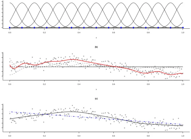
In Figure 4.1 we see a graphical representation of how P-splines work in practice. The top panel depicts a large B-spline base of degree p = 3 based on the set of knots (κ1, . . . , κk) represented by dots. B-splines of degree p are bell-shaped smooth curves,
(p−1) times differentiable, joined together at each knot point. For a given point of the
X domain, (p+ 1) B-splines have positive values and the B-spline base has a dimension
K =p+k+ 1.
as regression matrix in a GLM, taking η(x) = Bµαµ. Each B-spline j (j = 1, . . . , K) is
then multiplied by a certain amplitudeαµ,j, and the linear combination of these amplified
B-splines corresponds to the final estimate. In Figure 4.1 (b) the amplified B-splines are drawn as dashed lines, while the estimate that is obtained as their linear combination can be seen as a solid line. Clearly, since the regression matrix is so rich, the fit is too wiggly and it overfits the data. In order to avoid this overfitting, we add a difference order type of penalty which ensures that adjacent coefficients are not too different. Estimates forαµ
are obtained as the solution to: BTµ y−µ(x) φV(µ(x))µ ′ −λPµαµ =0, (4.1)
with Pµ an appropriate matrix representation of the difference operator (as in Eilers
and Marx (1996)). The smoothing parameter λ > 0 governs the balance between the overfitting and the smoothness of the fitted function. In Figure 4.1 (c) we see the effect of the smoothing parameter: the solid line is obtained with a moderate value for λ while the dashed-dotted line is obtained with a too large value for λ, leading to a too smooth estimate. In Section 5 we discuss methods to optimally choose the smoothing parameter. P-splines can be used also when we are interested in determining the relationship between the expected value of Y and more than one covariate. We take η(xd) = αµ,0 +
η1(x1) +. . .+ηd(xd) and fit the generic component ηj(xj) via P-splines. For a given
i.i.d. sample (x,y) we build d large B-spline base matrices Bµ,1, . . . ,Bµ,d and model
η(x) as a linear combination of the B-splines matrices η(x) = αµ,0 +Bµ,1αµ,1 +. . .+
Bµ,dαµ,d = Bµαµ, with Bµ = [1n,Bµ,1, . . . ,Bµ,d] a unique design matrix and αµ =
(αµ,0,αµ,1, . . . ,αµ,d) the unique vector of parameters to be estimated. In order to avoid
overfitting for each of the d components we build d penalty matrices Pµ,1, . . . ,Pµ,d and
take λµ = (λµ,1, . . . , λµ,d) a vector of smoothing parameters governing the smoothness
of the components. Taking Pµ = blockdiag[0, λµ,1Pµ,1, . . . , λµ,dPµ,d] a blockdiagonal
penalty matrix, we obtain an estimate of αµ as the solution of
BTµ y−µ(x) φV(µ(x))µ ′ −Pµαµ =0.
Gijbels and Prosdocimi (2010) further extended P-GAMs and present Double Gener-alized Additive Models to model both the mean and the dispersion function as flexible functions of the covariates. In the next section we combine this extended P-GAM set-ting with the robust EQL framework presented in Section 2 to obtain robust and smooth estimates for both the mean and the dispersion function.
0.0 0.2 0.4 0.6 0.8 1.0 0.0 0.2 0.4 0.6 (a) x Bsplines 0.0 0.2 0.4 0.6 0.8 1.0 −100 0 50 100 (b) x y 0.0 0.2 0.4 0.6 0.8 1.0 −100 0 50 100 (c) x y
Figure 4.1: P-splines in practice. (a) a B-spline base is shown; (b) the weighted B-splines (dashed lines) and the final fit obtained when using a large B-spline base (solid line). The effects of the smoothing parameter can be seen in (c).
4.2
Robust Extended P-GAM
We next allow the dispersion function to be a smooth function of the covariates, and we propose estimators that are smooth as well as robust against outliers. Again we use the EQL framework and make assumptions only on the first two moments of (Y|Xd = xd)
and (d(Y, µ)|Xd = xd) just as in (2.2) and (2.3). Once more, η(·) and ξ(·) are two link
functions for the mean and the dispersion respectively. These link functions are of the formη(xd) =αµ,0+η1(x1) +. . .+ηd(xd) and ξ(xd) = αγ,0+ξ1(x1) +. . .+ξd(xd), where
the ηj(xj) and ξj(xj) components are modelled via P-splines.
As in Section 4.1 for a given i.i.d. sample (x,y) we build the unique regression matrix Bµ and the blockdiagonal penalty matrix Pµ. In the same way we build the regression
matrix Bγ and, given a set of smoothing parameters λγ = (λγ,1, . . . , λγ,d), the penalty
Smooth and robust estimates for αµ and αγ are obtained as the solution to
Ψs(y, µ(x))−Pµαµ=BTµ(sψ(y, µ(x))w(x)µ′−a(αµ))−Pµαµ =0 (4.2)
and
Ψt(d, γ(x))−Pγαγ =BTγ (tψ(d, γ(x))w(x)γ′−b(αγ))−Pγαγ =0. (4.3)
These estimates can be shown to have a bounded influence function when Ψs(·,·) and
Ψt(·,·) are bounded, as in Section 3. Note how (4.2) and (4.3) differ from (3.1) and (3.3)
since nowBµ andBγ represent a larger combination of matrices, and there is the penalty
term which ensures the smoothness of the fit.
Estimates for αµ and αγ are obtained via iterative procedures. In particular the rule
to update the current estimate ˜αµ of αµ is:
αµ= (BTµW˜ µBµ+Pµ)−1BTµW˜ µz˜µ, (4.4) where ˜Wµ = diag −Eh d dαµΨs(Y,µ˜(Xd))|Xd=xd,i i i, ˜ zµ =Bµα˜µ+ ˜W −1 µ Ψs(y,µ˜(x))
and ˜µ(·) is the vector of current estimates forµ(·) which depends on ˜αµ. Similarly αγ is
updated with the following scheme:
αγ = (BTγW˜ γBγ+Pγ)−1BTγW˜ γz˜γ , (4.5) where ˜Wγ = diag −Eh d dαγΨt(d(Y, µ),γ˜(Xd))|Xd=xd,i i i, ˜zγ =Bγα˜γ+ ˜W −1 γ Ψt(d,γ˜(x))
and ˜γ(x) is the vector of current estimates for γ(x) which depends on ˜αγ.
Once convergence is reached we take ˆη(x) =Hµ(λµ)˜zµ, withHµ(λµ) =Bµ(BTµW˜ µBµ+
Pµ)−1BTµW˜ µ the hat matrix for the mean model which depends on the values of λµ.
Similarly we have ˆξ(x) = Hγ(λγ)˜zγ with Hγ(λγ) = Bγ(BTγW˜ γBγ +Pγ)−1BTγW˜ γ
the hat matrix for the dispersion model. Finally we take df(λµ) = tr(Hµ(λµ)) and
df(λγ) = tr(Hγ(λγ)) to be the equivalent number of degrees of freedom for the mean and
the dispersion model.
The general estimation procedure iterates between the two iterative estimation steps for αµ and αγ, as in Gijbels and Prosdocimi (2010). The smoothing parameters λµ and
λγ strongly influence the final appearance of the fits and are chosen before each of the
iterative steps, using methods discussed in the next section.
5
Smoothing parameter selection
The solution to (4.4) and (4.5) can be found via iterative methods, although the smooth-ness of the final estimate depends on the values of the smoothing parametersλµ andλγ.
Different methods for choosing the smoothing parameters exist. A standard procedure is to minimize the Generalized Cross Validation (GCV) criterion (Wahba (1990)):
GCV(λµ) =1Tn
d(y,µˆ(x,λµ))
(n−df(λµ))2
, (5.1)
where with ˆµ(x,λµ) we want to emphasize that the estimate of µ(x) depends on λµ.
The criterion above is widely used in standard GAMs to choose optimal values forλµ.
Nevertheless, the criterion needs to be slightly modified when the dispersion function is considered to be no longer constant as in Gijbels and Prosdocimi (2010). Moreover, as mentioned by Cantoni and Ronchetti (2001b), the choice of λµ via GCV will no longer
work well in presence of outliers, even when the estimation procedure is robust. Here we propose to choose optimal values for λµ via a robust version of GCV:
RGCV(λµ) = 1Tn
ψq(d(y,µˆ(x,λµ))/γ)
(n−df(λµ))2
.
where γ once more denotes the vector of estimated γ(·) values which is kept fixed when estimating the mean function.
The choice of smoothing parameters for the dispersion function is much less discussed in the literature. Gijbels and Prosdocimi (2010) propose an appropriate form of GCV for the choice of the λγ. Here, we propose to use a robustified version of this criterion:
RGCV(λγ) =1Tn
ψq(dγ(d,ˆγ(x,λγ)))
(n−df(λγ))2
.
where dγ(d,ˆγ(x,λγ)) is the vector of deviance residuals for the dispersion model, with
dγ(·,·) the deviance function defined as (see 2.1)
dγ(d, γ(xd)) = 2
Z d γ(xd)
d−t
2t2 dt . (5.2)
Akaike’s Information Criterion (AIC) is also often used to choose a smoothing parameter value (among others in the original Eilers and Marx paper (1996)). Similarly to what is done for GCV, AIC can also be appropriately modified for a robust selection of the smoothing parameters for both the mean and the dispersion function estimation. The two criteria to be minimized are then:
RAIC(λµ) =1Tnψq d(y,µˆ(x,λµ)) γ + 2 df(λµ), and RAIC(λγ) =1Tnψq(dγ(d,ˆγ(x,λγ))) + 2 df(λγ).
Simulation results not presented here show that in many cases the two criteria (AIC and GCV; and RAIC and RGCV) perform comparably.
In all the RGCV(·) and RAIC(·) criteria we take ψq to be the Huber function defined
in (3.2) with tuning constant q. Taking q = ∞ corresponds to using the standard GCV and AIC criteria. In our applications we take q to be equal to c, the value of the tuning constant in the estimating procedure, but other choices could be done. Also, bounded functions other than the Huber function could be employed both in the estimation and in the smoothing parameters selection.
6
Simulation study
We investigate the performance of the proposed method through a simulation study. We simulated 1000 datasets of size n = 250 coming from a Poisson-like distribution with mean function µ(x) = exp(η0 + η1(x1) +η2(x2)) and dispersion function γ(x) =
exp(ξ0+ξ1(x1) +ξ2(x2)) with:
η0 = 1, η1(x1) = 1.8 sin(3.4x21), η2(x2) = 1.1 cos(8x2)
ξ0 =−.35, ξ1(x1) = 2.3 sin(2x1)x21, ξ2(x2) =−1.35(sin(x2) exp(1.5−0.8x2)).
When summarizing the simulation results we present centered curves. This means that we subtract from a curve its average over the values taken in all data points, i.e. for example for η1(x1) we present η1(x1)−n−1Pni=1η1(x1,i). The covariates x1 and x2 are generated
from two independentU(0,1) distributions. We simulated data in three different settings, placing a growing percentage of outlying datapoints (0%, 3% and 5%) located in.1< x1 <
.2 and .8 < x2 < .9. In this Poisson-type modelling we take V(µ) = µ, and logarithmic
link functions for both the mean and the dispersion: η(·) = log(µ(·)) and ξ(·) = log(γ(·)). Also, we takew(·) = 1.
For each simulated dataset we estimated both the mean and the dispersion function via the Robust Extended GAM procedure proposed in Section 4 choosing the smoothing parameters both via the standard GCVs and the robust versions proposed in Section 5. We compare the performance of the proposed methods with the non-robust Extended GAM of Gijbels and Prosdocimi (2010) and the standard GAM with mean function estimation only. In this way we are able to investigate the differences between both robust and non-robust methods, and between models in which only the mean function is estimated and the Double models in which both the mean and the dispersion functions are estimated.
For a given dataset we evaluate the performance of the estimation procedure via the approximate integrated square error:
AISE = n X i=1 ˆ
f(xd,i)−ftrue(xd,i)
2 n X i=1 (ftrue(xd,i)) 2 ,
with ˆf(·) the estimated function and ftrue(·) the true function. In Figures 6.1 and 6.2
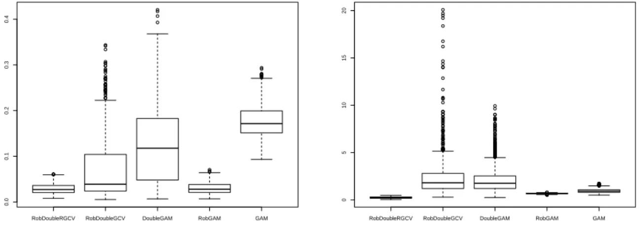
we summarize the results for the 0% and the 3% contamination setting. The results for the 5% contamination setting (not shown here) give results similar to these for the lower contamination setting. In each plot we show the boxplots of the AISE values for the mean and the dispersion function estimation for the different estimation procedures (boxplots from left to right):
• RobDoubleRGCV: the proposed robust estimation of mean and dispersion function,
with smoothing parameter chosen via RGCV;
• RobDoubleGCV: the proposed robust estimation of mean and dispersion function,
with smoothing parameter chosen via standard GCV;
• DoubleGAM:the non-robust estimation of mean and dispersion function as in Gijbels
and Prosdocimi (2010), with smoothing parameter chosen via GCV;
• RobGAM:the robust GAM estimation of the mean function, with smoothing
param-eter chosen via GCV;
• GAM:the standard GAM estimation of the mean function, with smoothing parameter
chosen via GCV;
From Figure 6.1 it is seen that in case of no contamination the non-robust and the robust methods have similar behavior, with non-robust methods performing slightly bet-ter. We note that not taking into account the variability in the dispersion function can have a bad influence on the mean estimation as well. From Figure 6.2 we can see that as soon as outliers are present in the data, the non-robust methods perform worse and worse: we even get lower AISE values for the dispersion when the dispersion function is not estimated rather than estimated in a non-robust way. Note also that choosing the smoothing parameters with a robust criterion plays a crucial role: when using robust methods the optimal smoothing parameters need to be chosen with a robust criterion as
RobDoubleRGCV RobDoubleGCV DoubleGAM RobGAM GAM
0.00
0.02
0.04
0.06
boxplots of AISE values for the mean
RobDoubleRGCV RobDoubleGCV DoubleGAM RobGAM GAM
0
1
2
3
4
boxplots of AISE values for the dispersion
Figure 6.1: The 0% contamination setting: boxplots of AISE values for the mean (left) and dispersion (right) estimation.
RobDoubleRGCV RobDoubleGCV DoubleGAM RobGAM GAM
0.0
0.1
0.2
0.3
0.4
boxplots of AISE values for the mean
RobDoubleRGCV RobDoubleGCV DoubleGAM RobGAM GAM
0
5
10
15
20
boxplots of AISE values for the dispersion
Figure 6.2: The 3% contamination setting: boxplots of AISE values for the mean (left) and dispersion (right) estimation.
well. In general the proposed method seem to perform quite well: not only the median AISE values are much lower than the ones of the other methods, but we also see little variability.
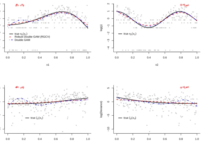
In Figure 6.3 we show a dataset simulated under the 3% contamination setting, to-gether with non-robust and robust estimates for the mean and dispersion functions. It is clearly seen that the robust methods are less affected by the presence of outliers in the data.
0.0 0.2 0.4 0.6 0.8 1.0 −4 −3 −2 −1 0 1 2 x1 log(y) true η1(x1)
Robust Double GAM (RGCV) Double GAM 0.0 0.2 0.4 0.6 0.8 1.0 −4 −3 −2 −1 0 1 2 x2 log(y) true η2(x2) 0.0 0.2 0.4 0.6 0.8 1.0 −10 −5 0 5 x1 log(De viance) true ξ1(x1) 0.0 0.2 0.4 0.6 0.8 1.0 −10 −5 0 5 x2 log(De viance) true ξ2(x2)
Figure 6.3: A simulated dataset from the 3% contamination setting. Outliers are indicated with crosses and estimates for both the mean (top panels) and the dispersion (lower panels) functions are superimposed.
7
Real data examples
In all examples we use a logarithmic link for the dispersion function, i.e. ξ(·) = log(γ(·)), and take w(·) = 1), i.e. no weighting function is employed to correct for leverage points.
7.1
Influenza-like Illness visits in the US
Alimadad and Salibian-Barrera (2009) study how the weekly counts of Influenza-like Ill-ness (ILI) visits in the US change in the course of the influenza season (which lasts 33 weeks, from week 40 to the end of week 20 of the next year). They analyze data regarding the influenza seasons of 2006/2007, 2007/2008 and 2008/2009. During the last weeks of the 2008/2009 season the H1N1 flu started spreading, and this resulted in a higher num-ber of visits. Therefore, they suggest to analyze the data using robust methods which
are less affected by the presence of high numbers of visits. What they do not take into account is that the variability of the data also seems to be changing over the weeks within the season. We propose that, to analyze these data properly, not only the mean but also the dispersion function should be estimated. The presence of extreme points in the data, suggests indeed that we should apply robust methods. For the mean modelling we take
V(µ) =µ and a logarithmic link function η(·) = log(µ(·)), as we would do for a Poisson regression.
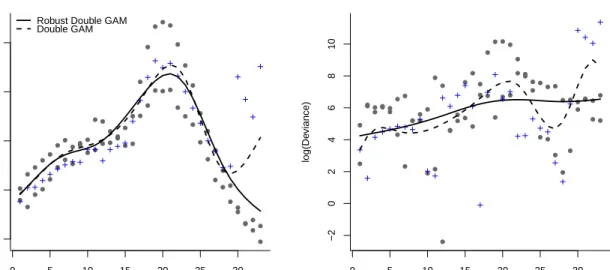
In the right panel of Figure 7.1 we present the centered (log) data with a robust and a non-robust fit of the mean, while the centered (log) deviance residuals with a fit for the ξ(weeks) component are shown in the right panel. We see that the robust methods are less affected by the presence of extreme values in the data, both for the mean and the dispersion estimation. We claim that the dispersion of the model should indeed be estimated as a function: in Figure 7.2 we see the standardized Pearson residuals we would obtain from a robust model with a constant dispersion (rP = (y−µ)/(φµ)) and the ones
we obtain when modelling also the dispersion in a robust way (rP = (y −µ)/(φγµ)).
Clearly the shape present in the residuals in the left plot diminishes when estimating the dispersion and we also notice how the outlying points at the extreme right of the plot have now lower residuals.
0 5 10 15 20 25 30 −1.0 −0.5 0.0 0.5 1.0 Weeks log(ILI visits)
Robust Double GAM Double GAM 0 5 10 15 20 25 30 −2 0 2 4 6 8 10 Weeks log(De viance)
Figure 7.1: ILI visits in the US (crosses indicate data of the 2008/2009 season): Ro-bust Double GAM (solid) and standard Double GAM (dashed line) fits for the mean and dispersion function.
0 5 10 15 20 25 30 0 5 10 Weeks standardiz ed residuals 0 5 10 15 20 25 30 0 5 10 Weeks standardiz ed residuals
Figure 7.2: Standardized residuals for the fits to the ILI visits. On the left the residuals obtained when taking the dispersion as a constant, on the right the ones obtained when taking the dispersion to be a function of the covariate.
A consequence of estimating the dispersion is that points which correspond to ex-tremely high ILI visit counts and that have very large residuals in the left plot are scaled by the estimated dispersion function, which has higher values in the area where the more extreme counts are observed. Indeed in the right panel of Figure 7.2 the points with higher residuals are less sticking out, they appear to be less extreme. If we think that the process under study is prone to have parts of larger variability we should estimate the dispersion function and allow the process to be more variable in some parts, rather than interpreting high counts automatically as outliers.
7.2
The ozone data
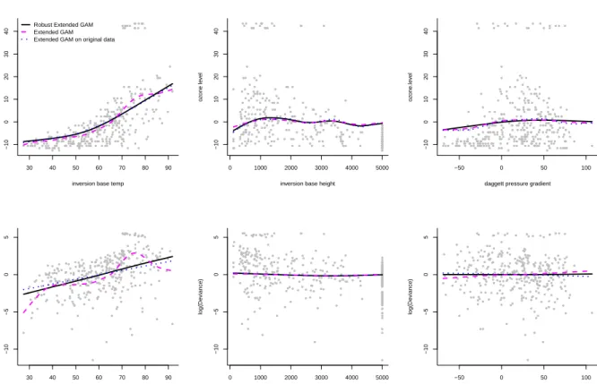
In Figure 7.3 (top panels) data on the ozone level in Upland, California in 1976 (see Breiman and Friedman (1985)) are depicted. We are interested in modelling the ozone level as a flexible function of the inversion base temperature, the inversion base height and the daggett pressure gradient. To illustrate what the effect of outliers can be, we replaced 5% of the data by outliers scattered uniformly around (55,58). The data points to be substituted by outliers were selected among those with inversion base temperature values between (70,80). We take V(µ) = 1 and the identity link η(·) = µ(·), the default
30 40 50 60 70 80 90 −10 0 10 20 30 40
inversion base temp
oz
one le
v
el
Robust Extended GAM Extended GAM Extended GAM on original data
0 1000 2000 3000 4000 5000 −10 0 10 20 30 40
inversion base height
oz one le v el −50 0 50 100 −10 0 10 20 30 40
daggett pressure gradient
oz one .le v el 30 40 50 60 70 80 90 −10 −5 0 5
inversion base temp
log(De viance) 0 1000 2000 3000 4000 5000 −10 −5 0 5
inversion base height
log(De viance) −50 0 50 100 −10 −5 0 5
daggett pressure gradient
log(De
viance)
Figure 7.3: The Ozone data with outliers: Robust Double GAM (solid) and non-robust Double GAM (dashed line) fits for the mean and the dispersion (top and bottom panels respectively). The dotted line represent the fit from a non-robust double estimation of the mean and dispersion function on the original data.
choice in standard GAM for data assumed to be Normal.
In Figure 7.3 we see how the robust techniques are much less influenced by the pres-ence of the outliers in the data. The robust estimates obtained for the mean and the dispersion function resemble indeed much more the shape we would get when outliers are not present in the data.
7.3
The Italian abortion data
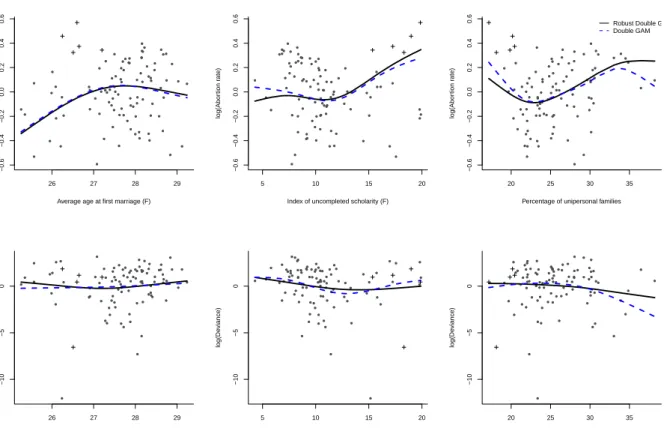
In Figure 7.4 data on the induced abortion rate for each Italian province are shown. This dataset was previously analyzed in Gijbels and Prosdocimi (2010). We are interested in studying how the abortion rate in the 98 Italian provinces changes as a function of the following socio-economical covariates:
26 27 28 29 −0.6 −0.4 −0.2 0.0 0.2 0.4 0.6
Average age at first marriage (F)
log(Abor tion r ate) 5 10 15 20 −0.6 −0.4 −0.2 0.0 0.2 0.4 0.6
Index of uncompleted scholarity (F)
log(Abor tion r ate) 20 25 30 35 −0.6 −0.4 −0.2 0.0 0.2 0.4 0.6
Percentage of unipersonal families
log(Abor
tion r
ate)
Robust Double GAM Double GAM
26 27 28 29
−10
−5
0
Average age at first marriage (F)
log(De viance) 5 10 15 20 −10 −5 0
Index of uncompleted scholarity (F)
log(De viance) 20 25 30 35 −10 −5 0
Percentage of unipersonal families
log(De
viance)
Figure 7.4: The abortion data: Robust Double GAM (solid lines) and standard Double GAM (dashed lines) fits for the mean and dispersion function (top and bottom panels respectively). Crosses indicate the provinces of Puglia.
• the average age at first marriage for women;
• the index of non-finished compulsory education for the female population between 15 and 52;
• the percentage of unipersonal families.
As Section in 7.1 we take V(µ) = µ and η(·) = log(µ(·)) in this example. Smoothing parameters for the standard and the robust fit are selected respectively via AIC and RAIC.
We know that the highest values present in the dataset are coming from the 5 provinces in one region (Puglia) in which the health care system, specially concerning induced abortion, is of higher quality than the one of the neighboring regions. It is suspected that the high abortivity rates observed in this region are due more to women from outside who travel to undergo the operation rather than from a real higher abortion rate among the women of the region. By using a robust estimate for the mean and dispersion value we
are assured that these outlying points will have less effect on the final estimates, as can be seen in Figure 7.4: indeed the robust fits are less affected by the presence of extreme points.
Acknowledgements
Support from the GOA/07/04-project of the Research Fund KULeuven is gratefully ac-knowledged, as well as support from the IAP research network nr. P6/03 of the Federal Science Policy, Belgium.
References
Alimadad, A. and Salibian-Barrera, M. (2009). An outlier-robust fit for Generalised Additive Models with applications to outbreak detection. Manuscript, available at the second author’s website.
Breiman, L. and Friedman, J. (1985). Estimating optimal transformations for multiple regression and correlation,Journal of the American Statistical Association,80, 580– 619.
Cantoni E. and Ronchetti E. (2001a). Robust Inference for Generalized Linear Models. Journal of the American Statistical Association, 96, 1022–1030.
Cantoni E. and Ronchetti E. (2001b). Resistant selection of the smoothing parameter for smoothing splines. Statistics and Computing, 11, 141–146.
Eilers, P.H.C. and Marx, B.D. (1996). Flexible Smoothing with B-splines and Penalties. Statistical Science,11, 89–121.
Gijbels I. and Prosdocimi I. (2010). Smooth estimation of mean and dispersion func-tion in extended Generalized Additive Models with applicafunc-tion to Italian Induced Abortion data. Manuscript.
Gijbels I., Prosdocimi I. and Claeskens, G. (2010). Nonparametric estimation of mean and dispersion functions in extended Generalized Linear Models. Test, to appear. DOI 10.1007/s11749-010-0187-1
Hampel F., Ronchetti E., Rousseeuw P. and Stahel W. (1986). Robust statistics: the approach based on influence functions. Wiley, New York.
Hastie, T. and Tibshirani, R. (1990). Generalized Additive Models. Chapman and Hall: New York.
Hinde, J. and Dem´etrio C.G.B. (1998). Overdispersion: Models and estimation. Com-putational Statistics & Data Analysis, 27, 151–170.
Marx, B.D and Eilers, P.H.C. (1998). Direct generalized additive modeling with penal-ized likelihood. Computational Statistics & Data Analysis,28, 193–209.
McCullagh, P. and Nelder, J.A. (1989). Generalized Linear Models, Chapman and Hall: London.
Nelder, J.A. and Pregibon, D. (1987). An extended quasi likelihood function. Biometrika,
74, 221–232.
Wahba, G. (1990). Spline Models for Observational Data. Philadelphia: SIAM.
Wedderburn, R. (1974). Quasi-likelihood functions, generalized linear models, and the GaussNewton method. Biometrika, 61, 439–447.