A smoothing approach for composite conditional gradient with nonsmooth loss

gradient with nonsmooth loss

Federico Pierucci, Zaid Harchaoui, J´

erˆ

ome Malick

To cite this version:

Federico Pierucci, Zaid Harchaoui, J´

erˆ

ome Malick. A smoothing approach for composite

con-ditional gradient with nonsmooth loss. [Research Report] RR-8662, INRIA Grenoble. 2014.

<hal-01096630>

HAL Id: hal-01096630

https://hal.inria.fr/hal-01096630

Submitted on 15 Jan 2015

HAL

is a multi-disciplinary open access

archive for the deposit and dissemination of

sci-entific research documents, whether they are

pub-lished or not.

The documents may come from

teaching and research institutions in France or

abroad, or from public or private research centers.

L’archive ouverte pluridisciplinaire

HAL, est

destin´

ee au d´

epˆ

ot et `

a la diffusion de documents

scientifiques de niveau recherche, publi´

es ou non,

´

emanant des ´

etablissements d’enseignement et de

recherche fran¸

cais ou ´

etrangers, des laboratoires

publics ou priv´

es.

0249-6399 ISRN INRIA/RR--8662--FR+ENG

RESEARCH

REPORT

N° 8662

June 2014

for composite conditional

gradient

with nonsmooth loss

RESEARCH CENTRE GRENOBLE – RHÔNE-ALPES Inovallée

with nonsmooth loss

Federico Pierucci

∗ †

, Zaid Harchaoui

∗

, Jérôme Malick

‡

Project-Teams LEAR and BiPoP

Research Report n° 8662 — June 2014 — 21 pages

Abstract: We consider learning problems where the non-smoothness lies both in the convex empirical risk and in the regularization penalty. Examples of such problems include learning with nonsmooth loss functions and atomic decomposition regularization penalty. Such doubly nonsmooth learning problems prevent the use of recently proposed composite conditional gradient algorithms for training, which are particularly attractive for large-scale applications. Indeed, they rely on the assumption that the empirical risk part of the objective is smooth.

We propose a composite conditional gradient algorithm with smoothing to tackle such learning problems. We set up a framework allowing to systematically design parametrized smooth surro-gates of nonsmooth loss functions. We then propose a smoothed composite conditional gradient algorithm, for which we prove theoretical guarantees on the accuracy. We present promising ex-perimental results on collaborative filtering tasks.

Key-words: conditional gradient, Frank-Wolfe, smoothing, large-scale convex optimization

∗ _{Inria, LEAR team, Inria Grenoble Rhône-Alpes, Laboratoire Jean Kuntzmann, CNRS, Univ. Grenoble}

Alpes, France.

†_{Univ. Grenoble Alpes, Laboratoire Jean Kuntzmann, CNRS, Inria Grenoble Rhône-Alpes, France.}

‡ _{CNRS, BIPOP team, Laboratoire Jean Kuntzmann, CNRS, Inria Grenoble Rhône-Alpes, Univ. Grenoble}

Contents

1 Introduction 3

2 Smooth optimization with atomic-decomposition regularization 4

3 Motivating example 5

4 Smoothing non-smooth loss functions 6

5 Smoothed Composite Conditional Gradient 8

6 Experiments 11

6.1 Implementation details . . . 11

6.2 Competing approaches . . . 12

6.3 Collaborative filtering . . . 12

7 Conclusion 13

A Properties of the B-conjugate 17

B Cited theorems 20

1

Introduction

The conditional gradient algorithm, a.k.a.Frank-Wolfe from the authors of the original paper

in 1956, performs smooth optimization over a compact convex set and only requires i) a first-order oracle and ii) a linear minimization oracle over that compact convex set. This historical algorithm and its recent extensions to different optimization formulations [JS10, HJN13, HK12, ZYS12, LJJSP13] are increasingly popular due to their relevance for large-scale applications. Applications include collaborative filtering on the Netflix dataset [JS10, SSGS11]. Related works also include greedy or forward selection algorithms [SSGS11], which can be considered as cousins to conditional gradient algorithms.

Indeed, conditional gradient algorithms stand in contrast to proximal algorithms for first-order optimization. For composite smooth optimization, proximal algorithms [BJMO12] require a first-order oracle that returns objective and gradient evaluations (for the smooth part), and a proximal operator oracle associated with the nonsmooth part of the objective. Such algorithms

are particularly attractive when the proximal operator is cheap to compute, as e.g. for the

vector`1-norm, and they enjoy anO(1/t2)convergence rate for their accelerated versions [JN10].

However, they could turn out to be prohibitive when the proximal operator is expensive if not

impossible to compute, e.g. for the nuclear-norm of matrices when these matrices are

high-dimensional, as it arises in the large-scale applications mentioned above. On the other hand, in place of the proximal operator oracle, conditional gradient algorithms (CGAs) require instead a

linear minimization oracle (LMO), which is much cheaper to compute,e.g. for the nuclear-norm

of matrices (maximal pair of singular vectors, in place of full SVD for the proximal operator). Composite conditional gradient algorithms, that is first-order optimization algorithms for composite objectives that decompose into a smooth part and a nonsmooth part for which a LMO is available, have been proposed [DHM12, HJN13, ZYS12]. Composite objectives correspond to

learning problems with smooth loss functions and nonsmoothregularization penalty. Convergence

learning context, these algorithms assume smooth loss functions, whereas for several applications nonsmooth loss functions would be preferable [WKLS07, AFSU07]. Smoothing strategies were recently proposed for nonsmooth counterparts of the “historical” conditional gradient algorithm, that is for nonsmooth objectives (instead of smooth in the original [Jag13]) with a compact convex constraint [Lan, GH13].

We propose here a smoothed version of the composite conditional gradient algorithm, using the smoothing technique from [Nes05]. We give a detailed study of smoothing of nonsmooth loss functions in a machine learning context, and give theoretical grounding for several popular smoothed counterpart of nonsmooth loss functions. We prove a theoretical guarantee on the accuracy of the solution given by our algorithm and present promising experimental results on collaborative filtering.

2

Smooth optimization with atomic-decomposition

regular-ization

In this section, we recall the main properties of atomic-decomposition norms, and then describe composite conditional gradient algorithms [DHM12, HJN13, ZYS12], which are tailored for learn-ing problems with these norms, as regularizers.

Learning with atomic-decomposition norms Consider a sequence ofi.i.d.examplesu1, . . . , uN,

and a loss function`(W, u). DenoteRemp(W) = 1/NP

N

i=1`(W, ui)the corresponding empirical

risk. In this paper, we consider regularized learning problems that write as

min

W g(W) :=λkWkA+Remp(W) (1)

wherek·kAis a so-called atomic-decomposition norm [CRPW12, DHM12]. Atomic-decomposition

norms (or atomic norm, in short) can be defined by the following simple variational description

with respect to a compact setA(the “atoms”). Assume that the elements ofAare the extreme

points of conv(A)(the convex hull ofA), we have

kWkA= inf ( X i∈I θi : θi>0, W= X i∈I θiai )

whereIis an index set spanning the elements ofA, and where(ai)i∈I ∈ A. Such characterization

leverages the property that norms belong to the larger family of “gauges”, that are convex and positively homogeneous functions, centered in the origin. The support function of the collection

of atomsAwrites as

kWk∗_A= sup

a∈A

hW, ai. (2)

We can recognize thatk · k∗

Ais the dual (or polar) norm associated withk · kA.

Many useful atomic norms enjoy collections of atoms A that are simple to describe, and

whose support functions arecomputationally easy to compute. Examples include the`1-norm in

Rd, whereAis the canonical basis of Rd, and the trace-norm (or nuclear-norm) in the space of

rectangular matricesRd×k, whereA={uvT, kuk2=kvk2= 1}. We refer to [Jag13] for a review

of popular atomic norms.

Conditional gradient algorithms, which we shall describe in the next paragraph, take advan-tage of this attractive feature: they make progress using an (approximated) optimal solution of (2).

Composite conditional gradient for smooth risk Assume that the empirical riskRemp(·)

is a convex function with Lipschitz continuous gradient with Lipschitz constantL. Under suitable

assumptions [HJN13], the composite conditional gradient algorithm with infinite memory enjoys the following theoretical guarantee

g(Wt)−min W g(W)≤O ₁ t .

The composite conditional gradient algorithm works by making calls to afirst-order oracle, that

returns Remp(W) and ∇Remp(W) for any W, and to a linear minimization oracle, that is a

subroutine that returns for anyW

LMO(W) := argmin

a∈A

ha,∇Remp(W)i. (3)

This is in contrast to proximal algorithms, which make progress by making calls to aproximal

op-erator oracle. Proximal operators are computationally expensive to compute in several large-scale

learning problems. Typical examples are matrix completion with noise, or multi-class classifica-tion with nuclear-norm penalty, where the proximal operator associated with the nuclear-norm corresponds to a full singular value decomposition of the current iterate, which is prohibitive in large-scale applications. Moreover, recent results from [GN13] show that the conditional gradient

algorithm, which runs inO(1/t), as opposed to the accelerated proximal algorithms which run

in O(1/t2), is almost optimal (up to a log factor) for large-scale optimization problems.

The composite conditional gradient algorithm is summarized below (see Algo. 1). An

-solution is aW that satisfies

(i) k∇Remp(W)kA≤λ+, and

(ii) |h∇Remp(W), Wi+λkWkA| ≤kWkA.

Algorithm 1Composite Conditional Gradient Inputs: λ,

InitializeW =0,t= 1

whileW is not an-solutiondo

Call the linear minimization oracle: LMO(Wt)

Compute min θ1,...,θt≥0 λ t X i=1 θi+Remp Xt i=1 θiai Incrementt←t+ 1 end while ReturnW =P iθiai

3

Motivating example

We present here collaborative filtering as motivating example for designing a composite con-ditional gradient algorithm for matrix learning problems with nonsmooth loss functions. The (nonsmooth) regularization is the nuclear-norm, the sum of singular values of the matrix, which

has an atomic-decomposition formk·k_A with

Collaborative filtering, or matrix completion, consists in the generation of a low-rank matrix

from few known approximate entries. The loss `(w, x) = |w−x|, based on `1 norm [Hub81]

ensures robustness to outliers. We have (1)

min W∈Rd×k 1 N X (i,j)∈Ω |Wij−Xij|+λkWk_A (4)

whereΩis the subset of {1, . . . , d} × {1, . . . , k} denoting pairs of observations (N is the size of

Ωand {xij}(i,j)∈Ω are the known entries).

4

Smoothing non-smooth loss functions

The smoothing technique that we consider in this paper was formalized, for the accelerated gradient method, by Nesterov [Nes05, Nes07]; see also [Ber04] for a review of earlier works. We study in greater detail this smoothing for the specific purpose of smoothing loss functions considered in learning problems. In this section, we give a short and comprehensive presentation of this smoothing technique applied to support functions, revealing a convex transformation generalizing the standard convex conjugation [HUL01].

Ball-conjugate Letγ > 0, a set B ⊂Rn and a function f: B →R∪ {+∞}. Note that, for

the study of this section, the variable of functionf isx.

We introduce theB-conjugate off of parameterγto be the function defined for allsin Rn

by

(γf)B(s) := max

x∈B

x∈domf

hx, si −γf(x). (5)

As a maximum of affine function, (γf)B is convex function. When γ = 1 and B = Rn, the

B-conjugate is nothing but the traditional convex conjugate: fB=f∗(see Chap. E of [HUL01]).

In general, we see on definitions that theB-conjugate off is the convex conjugate ofγfrestricted

toB,

(γf)B= γf_|B∗

(6)

wheref|B is the restriction of f onB.

The ball-conjugate inherits some (but not all) properties of the convex conjugate.

Outstand-ingly, the Fenchel inequality still holds : for allx∈ B

s∈∂f(x) ⇔ fB(s) +f(x) =hs, xi. (7)

Observe also that, by definition, theB-conjugate of the constant zero function (denoted0:s7→0)

is the called support function ofB

∀s∈_Rn _σ

B(s) =0B(s).

In the next section, we state the two properties of the ball-conjugate with respect to smooth approximations. Other properties, including many useful calculus rules, are presented in supple-mentary material.

Smooth approximation of support functions We show here that ball-conjugation gives an easy, constructive and controllable way to approximate, by smooth functions, the support

function ofB

σ(s) = max

x∈B hs, xi.

The next two theorems show the main results of the approximation. Letf be a convex function

andBa convex compact set.

Theorem 4.1 (Approximation). Consider the lower and upper bounds on B: m ≤f(x)≤M

for allx∈ B. Then, for s∈Rn

γm≤σ(s)−(γf)B(s)≤γM.

Theorem 4.2(Smoothing). Assumef to be strongly convex with constantc onB. Then(γf)B

is differentiable on _Rn _{and its gradient}

∇(γf)B(s) = argmax

x∈B

hs, xi −γf(x)

is Lipschitz continuous on Rn with constantL= 1/γc.

In words, any strongly convex functionf generates, through itsB-conjugate, a smooth

ap-proximation of the support function of B. In general, the choice of f would depend on the

capability on computing easily itsB-conjugate and on the geometry ofBto control the constants

mandM. In the next section, we explicit computation with the squared euclidean norm. Other

examples are given in appendix. Ball-conjugate of `2

2-norm in [−1,1] Smooth functions generated by the squared euclidean

norm have explicit form involving the projection operator ontoB

πB(y) = argmin

x∈B

kx−yk2₂ .

Proposition 4.3. Let γ > 0 and B convex compact set. TheB-conjugate of f(·) = 1₂k·k2₂ can be expressed (γf)B(s) =DπB 1 γs , sE−γ 2 πB 1 γs 2 2. Its gradient is ∇(γf)B(s) =πB _s γ .

In addition(γf)B has Lipschitz constant L= 1/γ.

Smooth function based on the`2

2-norm would be interested only if the projectionπB is fast

to compute. The next example provides an illustration that will be used in the next section.

Consider inRthe setB= [−1,1], whose support function is just the absolute valueσ=|·|. By

the previous proposition, the conjugate of the squared norm is forsin _R

(γf)B(s) =s·π[−1,1] _s γ −γ 2 π[−1,1] _s γ 2 . (8)

In this simple example, the projection is explicit and we have

(γf)B(s) =

( ₁ 2γs

2 _{if |s| ≤γ}

We observe that we have the global approximation0 ≤ |s| −(γf)B(s)≤ γ₂ , as shown in Thm.

4.1. and that the function is smooth, as predicted by Thm 4.2. Note finally that

∇(γf)B(s) =      1 if s > γ 1 γs if |s| ≤γ −1 if s <−γ . (10)

Application to the motivating example We show how the smoothing technique can be applied to the nonsmooth empirical loss of collaborative filtering with noise. We approximate the absolute value in the empirical risk of problem (4) by the smooth conjugate of (9) that we denote

`γ(Wij, Xij) = (γf)B(Wij−Xij).

For given smoothing parameterγ, we thus consider the smooth surrogate learning problem

min W 1 N X (i,j)∈Ω `γ(Wij, Xij) +λkWk_A. (11)

The empirical risk of this problem is now smooth and we have a explicit expression of its gradient

by Eqn. (10). For any(i, j)∈Ω

(∇Rγ_emp(W))ij=

1

N∇Wij`

γ_(W

ij, Xij). (12)

5

Smoothed Composite Conditional Gradient

We present here the proposed algorithm, termedSmoothed Composite Conditional Gradient and

abbreviated SCCG in the remainder of the paper.

Smoothing the empirical risk In the motivating example, the empirical riskRemp(W)

(ab-breviatedR(W)from now on) is an empirical average over all the examples of somenonsmooth

loss function R(W) = 1 N N X i=1 `(W, ui)

where`is a support function precomposed with an affine operator:

`(W, ui) := max

x∈BhA(W, ui), xi.

We wrote the loss function in a compact form, to be understood as an abstract form that can be represent also (among others) our motivating example. Thanks to the smoothing technique, we

can now design asmoothed versionRγ_{(W)of the empirical risk, parameterized by a smoothing}

parameterγ that controls the amount of smoothing.

Rγ(W) = 1 N N X i=1 `γ(W, ui) where `γ(W, ui) := max x∈BhA(W, ui), xi −γf(x).

By Proposition 4.2,Rγ_{(·)is differentiable with Lipschitz continuous gradient. Therefore, one can}

use the composite conditional gradient algorithm presented earlier to solve the smooth optimiza-tion problem

min

W g

γ_{(W) :=λkWk}

A+Rγ(W). (13)

However, assuming that a solution to this problem is found by the composite conditional gradient algorithm

Wγ:= argmin

W

gγ(W)

it is yet to be determined how this solution deviates from the solution of the original problem (1).

The next proposition gives an insight on this issue, with notation of the previous section.

m, M andc are coming for the smoothing (see Theorems 4.1 and 4.2).

Proposition 5.1. Assume that γ ∈ [0, γmax]. In addition, assume that, for all γ ∈ [0, γmax],

there exists Dsuch thatλr+Rγ_(W)≤Rγ_{(0)together with kWk}

A≤rimply thatr≤D. Then,

setting

γ() = 2(M−m) ,

we have that, after

T()≥ _16D2

γc −13

iterations, for a sufficiently small accuracy, the SCCG algorithm returns an-optimal minimum of g.

Proof. We decompose the difference into three parts

g(Wt)−min W g(W)≤g(Wt)−g γ_(W t) +gγ(Wt)−min W g γ_(W) + min W g γ_(W)−min W g(W)

With the assumption, we can use the convergence rate of the composite conditional gradient with smooth loss (see Thm. 3 in [HJN13]): we get that

gγ(Wt)−min W g

γ_(W)≤ 8LγD2

t+ 14

where Lγ is the Lipschitz constant of the gradient. Here Lγ = 1/γcby Theorem 4.2. On the

other hand, we have from Theorem 4.1

g(Wt)−gγ(Wt)≤γM and min W g γ_(W)−min W g(W)≤ −γm

Therefore, to get an-optimal minimum ofg, it suffices to setγ=γ()and to runT()iterations

The above proposition can be interpreted as follows. Given a target accuracy, the optimal

amount of smoothing γ() can be computed so that after some number of iterations T() an

-optimal minimum of the objective function of interestgis reached.

The smoothed composite conditional gradient algorithm (SCCG) is summarized in Algo. 2.

The SCCG algorithm works by making calls to a first-order oracle, that returns Rγ_emp(W) and

∇Rγemp(W)for anyW, and to a linear minimization oracle, that is a subroutine that returns for

anyW

LMOγ(W) := argmin

a∈A

ha,∇Rγemp(W)i. (14)

Algorithm 2Smoothed Composite Conditional Gradient Inputs: λ,γ,

InitializeW =0,t= 1

fort= 1, . . . , T()do

Call the linear minimization oracle: LMOγ(Wt)

Compute min θ1,...,θt≥0 λ t X i=1 θi+Rγemp t X i=1 θiai ! end for ReturnW =P iθiai 0 500 1000 1500 0.01 0.1 1 time Empirical risk on train set, λ=1e−05

SCCG, γ= 0.5 Subgradient 0 50 100 150 200 250 300 0.01 0.1 1 iterations Empirical risk on train set, λ=1e−05

SCCG, γ= 0.5 Subgradient 0 1000 2000 3000 4000 0.25 0.39 0.63 0.25 0.39 time Empirical risk on train set, λ=1e−05

SCCG, γ = 0.5 Subgradient 0 10 20 30 40 50 60 0.25 0.39 0.63 iterations Empirical risk on train set, λ=1e−05

SCCG, γ = 0.5 Subgadient

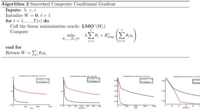
Figure 1: Comparison of empirical risk vs time (left of each box) and vs iterations number (right);

γ= 0.5λ= 10−5_{, on MovieLens datasets: the small dataset for the two figures on the left-hand}

side, the medium dataset for the two on the right-hand side.

Learning the smoothing parameter The optimal smoothing parameter γ() depends on

data-dependent quantities and requires some prior knowledge. Furthermore, the above result

only gives insights on the optimal amount of smoothing in terms optimization of the empirical

risk, whereas in real-world applications one is mainly interestedin fine in the risk on the test

set. In the experiments section, we see that an effective strategy would be tolearn the smoothing

parameter γ from data on a validation set. One would run the proposed algorithm SCCG(γ)

for all the values of γ ranging on a discretized set, and measure the validation error for each

value ofγon a held-out validation set. Then, one would pick the bestγin terms of error on the

validation set. With that learned valueγ?_{, one finally computes the test error obtained by the}

Train set

Validation set

Test set

Mo

v.

small

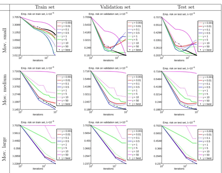
100 102 0.0113 0.0259 0.0592 0.1352 0.3089 0.7057 iterations Emp. risk on train set, λ=10−6

γ = 0.001 γ = 0.01 γ = 0.1 γ = 0.5 γ = 1 γ = 5 γ = 10 γ = 50 γ = best 100 102 0.191 0.248 0.3221 0.4183 0.5433 0.7056 iterations Emp. risk on validation set, λ=10−6

γ = 0.001 γ = 0.01 γ = 0.1 γ = 0.5 γ = 1 γ = 5 γ = 10 γ = 50 γ = best 100 102 0.2037 0.2613 0.3351 0.4298 0.5513 0.7072 iterations Emp. risk on test set, λ=10−6

γ = 0.001 γ = 0.01 γ = 0.1 γ = 0.5 γ = 1 γ = 5 γ = 10 γ = 50 γ = best

Mo

v.

medium

100 102 0.1451 0.1997 0.2748 0.3782 0.5204 0.7162 iterations Emp. risk on train set, λ=10−6

γ = 0.001 γ = 0.01 γ = 0.1 γ = 0.5 γ = 1 γ = 5 γ = 10 γ = 50 γ = best 100 102 0.188 0.2457 0.3211 0.4196 0.5484 0.7167 iterations Emp. risk on validation set, λ=10−6

γ = 0.001 γ = 0.01 γ = 0.1 γ = 0.5 γ = 1 γ = 5 γ = 10 γ = 50 γ = best 100 102 0.1883 0.246 0.3214 0.4198 0.5484 0.7164 iterations Emp. risk on test set, λ=10−6

γ = 0.001 γ = 0.01 γ = 0.1 γ = 0.5 γ = 1 γ = 5 γ = 10 γ = 50 γ = best

Mo

v.

large

100 101 0.2284 0.2859 0.358 0.4482 0.5611 0.7025 iterations Emp. risk on train set, λ=10−9

γ = 0.001 γ = 0.01 γ = 0.1 γ = 0.5 γ = 1 γ = 5 γ = 10 γ = 50 γ = best 100 101 0.2372 0.2947 0.3662 0.455 0.5654 0.7025 iterations Emp. risk on validation set, λ=10−9

γ = 0.001 γ = 0.01 γ = 0.1 γ = 0.5 γ = 1 γ = 5 γ = 10 γ = 50 γ = best 100 101 0.237 0.2945 0.366 0.4548 0.5652 0.7023 iterations Emp. risk on test set, λ=10−9

γ = 0.001 γ = 0.01 γ = 0.1 γ = 0.5 γ = 1 γ = 5 γ = 10 γ = 50 γ = best

Figure 2: Movielens data - Empirical risk versus iterations.

6

Experiments

We now present the experimental results of the proposed composite conditional gradient algo-rithm for the learning problem of collaborative filtering with noise, on the MovieLens datasets, with nuclear norm penality and nonsmooth loss function. The experiences are launched on 3 disjoint sets for train, validation, test.

We choseγ ∈ {0.001; 0.01; 0.1; 0.5; 1; 5; 10; 50} ; λ∈ {10−2; 10−4; 10−6; 10−8; 10−10; 10−12} .

For each λthe bestγλ is chosen as the one that minimizes the empirical risk on validation set

at last iteration. The pair (λbest, γbest ) minimizes the empirical risk on validation set at last

iteration. We chose as stop criterion a fixed number of iterations.

6.1

Implementation details

We implement our algorithm SCCG in Matlab. We use the quasi-Newton solver L-BFGS-B

[BLNZ95] (via a Matlab interface) to perform, at iteration tof our algorithm, the minimization

To deal with large scale data, we pay attention to the memory to store theWtgenerated by

the algorithm. EachWt is represented as a set containing the vectors ut, vt of each atomsat,

of length N, and coefficients θ. An object of the form {(uj, vj, θj)}j=1...t is stored at iteration

t. With T the maximum number of iterations, the memory to store all the iterations is then

proportional to T(T+1)

2 (2N+ 1).

Let us add a remark about the memory used for computations for movielens. Even though

eachWtis a dense matrix of dimensiond×k, we are interested only in its observed entries for

the optimization. So,Wtis never created as matrix object, but we keep only a representation of

it with a vector of entries and a vector of indices of lengthn. So we use onlyndoubles instead

ofdk. The only time we need a matrix of sized×kis to compute the descent direction, but this

matrix corresponds to the gradient of the loss and is sparse.

6.2

Competing approaches

A direct approach to solve out problem (1) would be to use standard nonsmooth optimization algorithms, namely bundle-like methods (see [HUL01]) or subgradient-like methods (see [Nes04], including proximal methods interpreted as implicit subgradient methods). Each iteration of

these methods requires the knowledge of a subgradient of the entire objective function g (or

at least an approximation of a subgradient). For many standard empirical losses, as the one used in this paper, a subgradient is readily available. There also exists an explicit expression

of the subdifferential of the trace-norm: we get a subgradient of the trace-norm atW from an

SVD decomposition of W, see [Lew99]. This is a bottleneck in scaling such approach to large

dimension: for the large-scale learning problem we consider, even computing a single SVD (then a single iteration of a nonsmooth optimization algorithm) is out-of-reach in a reasonable amount of time.

To illustrate this fact on collaborative filtering problems, we compare the SCCG algorithm

with fixedγ with a tailored basic nonsmooth optimization: truncated subgradient descent. An

iteration of this algorithm iteration writes Wk+1 = Wk +tkGk with Gk approximates a

sub-gradient in∂g(Wk). We compute only the 100 largest singular values to construct Gk to save

computing time. The comparaison of the decrease of the nonsmooth empirical risk is plotted in Figure 1. We see that for the small dataset the decrease of the subgradient method is better with respect of iterations and time, but that the situation is reversed for the medium-scale problems (and become even non-comparable for large-scale problems, not shown here). This confirms the discussion above about the prohibitive cost of computing a (even a poorly approximate of a) subgradient.

Again, more efficient algorithm as bundle methods would suffer from the same drawback: even though the algorithms are performant, they use information given by an oracle which over-costly for the problems we consider.

6.3

Collaborative filtering

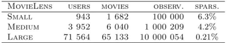
Dataset We test our approach on the MovieLens dataset for collaborative filtering, described

in [MAL+_{03]. This dataset contains evaluations of movies made by customers, represented by}

the sparse matrixX ∈_Rd×k_{. As every customer evaluated only a small number the movies, X}

is sparse. Here completing X means predict how a customer would evaluate a movie which he

hasn’t seen. Entries ofX are normalized dividing by the max entry ofX. We split the dataset

into a training set, validation and test sets with respectively60%,20%,20%of the entries. The

number of users and movies in the MovieLens datasets are resp. (943; 11,682) for the small,

Table 1: Data used for Collaborative Filtering. Sparsity is observations divided by total number of entries.

MovieLens users movies observ. spars. Small 943 1 682 100 000 6.3% Medium 3 952 6 040 1 000 209 4.2% Large 71 564 65 133 10 000 054 0.21%

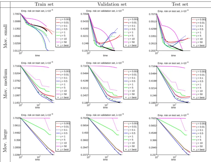
Results The plots with the nonsmooth empirical risk show better performance for medium γ

values. Whenγgets smaller we have a better approximation of the empirical risk, but the larger

Lipschitz constant L= 1/γ slows down the convergence of the algorithm. Whenγ gets larger

the approximation of the empirical risk gets worst. We recall that we obtain iterates with SCCG optimizing the smooth surrogate, but we plot the values of nonsmooth loss for those iterates. In

fig 3 and 2 we see the performance for allγwith the best choice of λ.

7

Conclusion

We proposed a composite conditional gradient algorithm that is suitable for regularized learn-ing problems with nonsmooth loss functions, and showed promislearn-ing experimental results. The framework we used allows to build smoothed counterparts of nonsmooth loss functions in a

prin-cipled manner, with theoretical guarantees on the accuracy with respect to the orignal doubly

Train set

Validation set

Test set

Mo

v.

small

100 0.0113 0.0259 0.0592 0.1352 0.3089 0.7057 time Emp. risk on train set, λ=10−6

γ = 0.001 γ = 0.01 γ = 0.1 γ = 0.5 γ = 1 γ = 5 γ = 10 γ = 50 γ = best 100 0.191 0.248 0.3221 0.4183 0.5433 0.7056 time

Emp. risk on validation set, λ=10−6 γ = 0.001 γ = 0.01 γ = 0.1 γ = 0.5 γ = 1 γ = 5 γ = 10 γ = 50 γ = best 100 0.2037 0.2613 0.3351 0.4298 0.5513 0.7072 time Emp. risk on test set, λ=10−6

γ = 0.001 γ = 0.01 γ = 0.1 γ = 0.5 γ = 1 γ = 5 γ = 10 γ = 50 γ = best

Mo

v.

medium

100 102 0.1451 0.1997 0.2748 0.3782 0.5204 0.7162 time Emp. risk on train set, λ=10−6

γ = 0.001 γ = 0.01 γ = 0.1 γ = 0.5 γ = 1 γ = 5 γ = 10 γ = 50 γ = best 100 102 0.188 0.2457 0.3211 0.4196 0.5484 0.7167 time

Emp. risk on validation set, λ=10−6 γ = 0.001 γ = 0.01 γ = 0.1 γ = 0.5 γ = 1 γ = 5 γ = 10 γ = 50 γ = best 100 102 0.1883 0.246 0.3214 0.4198 0.5484 0.7164 time Emp. risk on test set, λ=10−6

γ = 0.001 γ = 0.01 γ = 0.1 γ = 0.5 γ = 1 γ = 5 γ = 10 γ = 50 γ = best

Mo

v.

large

100 102 0.2284 0.2859 0.358 0.4482 0.5611 0.7025 time Emp. risk on train set, λ=10−9

γ = 0.001 γ = 0.01 γ = 0.1 γ = 0.5 γ = 1 γ = 5 γ = 10 γ = 50 γ = best 100 102 0.2372 0.2947 0.3662 0.455 0.5654 0.7025 time

Emp. risk on validation set, λ=10−9 γ = 0.001 γ = 0.01 γ = 0.1 γ = 0.5 γ = 1 γ = 5 γ = 10 γ = 50 γ = best 100 102 0.237 0.2945 0.366 0.4548 0.5652 0.7023 time Emp. risk on test set, λ=10−9

γ = 0.001 γ = 0.01 γ = 0.1 γ = 0.5 γ = 1 γ = 5 γ = 10 γ = 50 γ = best

References

[AFSU07] Y. Amit, M. Fink, N. Srebro, and Shimon Ullman. Uncovering shared structures in

multiclass classification. InICML, 2007.

[Ber04] D. Bertsekas. Nonlinear Programming (2nd ed.). Athena Scientific, 2004.

[BJMO12] F. R. Bach, R. Jenatton, J. Mairal, and G. Obozinski. Optimization with

sparsity-inducing penalties. Foundations and Trends in Machine Learning, 4(1):1–106, 2012.

[BLNZ95] R. H. Byrd, P. Lu, J. Nocedal, and C. Zhu. A limited memory algorithm for bound

constrained optimization. SIAM Journal on Scientific Computing, 16(5):1190–1208,

1995.

[CRPW12] V. Chandrasekaran, B. Recht, P. A. Parrilo, and A. S. Willsky. The convex geometry

of linear inverse problems. FOCM, 12(6):805–849, 2012.

[DHM12] M. Dudik, Z. Harchaoui, and J. Malick. Lifted coordinate descent for learning with

trace-norm regularization. Proceedings of the 15th International Conference on

Ar-tificial Intelligence and Statistics (AISTATS), 2012.

[GH13] D. Garber and E. Hazan. A Linearly Convergent Conditional Gradient Algorithm

with Applications to Online and Stochastic Optimization.ArXiv e-prints, 1301.4666,

2013.

[GN13] C. Guzman and A. Nemirovski. On Lower Complexity Bounds for Large-Scale

Smooth Convex Optimization. ArXiv e-prints, 1307.5001, 2013.

[HJN13] Z. Harchaoui, A. Juditsky, and A. Nemirovski. Conditional Gradient Algorithms for

Norm-Regularized Smooth Convex Optimization. ArXiv e-prints, 1302.2325, 2013.

[HK12] E. Hazan and S. Kale. Projection-free online learning. InICML, 2012.

[Hub81] P. J. Huber. Robust statistics. Wiley Series in Probability and Mathematical

Statis-tics. J. Wiley, 1981.

[HUL01] J.B. Hiriart-Urruty and C. Lemarechal. Fundamentals of Convex Analysis. 2001.

[Jag13] M. Jaggi. Revisiting Frank-Wolfe: Projection-free sparse convex optimization. In

ICML, pages 427–435, 2013.

[JN10] A. Juditsky and A. Nemirovski. First order methods for nonsmooth convex

large-scale optimization.Optimization for Machine Learning,(Sra, Nowozin, Wright, Eds),

MIT Press, 2012, 2010.

[JS10] M. Jaggi and M. Sulovský. A Simple Algorithm for Nuclear Norm Regularized

Problems. ICML 2010: Proceedings of the 27th international conference on Machine

learning, 2010.

[Lan] G. Lan. The Complexity of Large-scale Convex Programming under a Linear

Opti-mization Oracle. ArXiv e-prints, 1302.2325.

[Lew99] A.S. Lewis. Nonsmooth analysis of eigenvalues.Mathematical Programming, 84(1):1–

[LJJSP13] S. Lacoste-Julien, M. Jaggi, M. Schmidt, and P. Pletscher. Block-Coordinate

Frank-Wolfe Optimization for Structural SVMs. InICML 2013, 2013.

[MAL+_{03] B. Miller, I. Albert, S. K. Lam, J. Konstan, and J. Riedl. Movielens unplugged:}

Experiences with a recommender system on four mobile devices. InACM SIGCHI

Conference on Human Factors in Computing Systems, 2003.

[Nes04] Y. Nesterov.Introductory lectures on convex optimization: A basic course. Springer,

2004.

[Nes05] Y. Nesterov. Smooth minimization of non-smooth functions.Math. Program., 103(1),

2005.

[Nes07] Y. Nesterov. Smoothing technique and its applications in semidefinite optimization.

Math. Program., 110(2):245–259, 2007.

[SSGS11] S. Shalev-Shwartz, A. Gonen, and O. Shamir. Large-Scale Convex Minimization with

a Low-Rank Constraint. InICML, 2011.

[WKLS07] M. Weimer, A. Karatzoglou, Q. V. Le, and A. J. Smola. Cofi rank - maximum margin

matrix factorization for collaborative ranking. InNIPS, 2007.

[ZYS12] X. Zhang, Y. Yu, and D. Schuurmans. Accelerated training for matrix-norm

Appendix

Federico Pierucci, Zaid Harchaoui, Jérôme Malick

June 15, 2014

A

Properties of the B-conjugate

In this section, we give the proofs of the results about theB-conjugate, stated in the paper. We

also add a couple of useful lemmas. Our developments rely on basic convex analysis; for the reader convenience, the main results we need are recalled in Section B.

We start with proving that the approximation of the support function ofBby theB-conjugate

comes directly from its construction.

Proof. (of Thm. 4.1) The boundsm≤f(·)≤M yield that, for all x∈ B ands∈Rn

γm+hx, si −γf(x)≤ hx, si ≤γM+hx, si −γf(x)

Taking the max overx∈ B gives for alls∈Rn

γm+ (γf)B(s)≤σB(s)≤γM+ (γf)B(s)

which permits to conclude.

It is important for our approach to have some calculus rules to construct functions (γf)B.

Suppose we know the explicit formula forfB, we derive expression for theB-conjugate ofγf and

of the sum of f and an affine function.

Proposition A.1. For anyγ >0,b∈Randk∈Rn, we have:

(γf)B(s) =γfB_γ1s (15)

(f+h·, ki+b)B(s) =fB(s−k)−b (16)

Proof. (of Prop. A.1) We just develop from the definitions:

(γf)B(s) = max x∈Bhx, si −γf(x) =γmax x∈B 1 γhx, si −f(x) =γfBs_γ. In a similar way: (f+h·, ki+b)B(s) = max x∈Bhx, si − hx, ki −f(x)−b = max x∈Bhx, s−ki −f(x)−b =fB(s−k)−b.

We now turn to the smoothness of theB-conjugate. In what follows,Bis a convex compact

set, andf is a closed convex function onB. We also introduce

x∗(s) := argmax

x∈B

hs, xi −γf(x),

whose dependence onB,f andγ is implicit when obvious.

Lemma A.2. Let f be strictly convex onB; thenfB is differentiable on Rn and

∇fB(s) =x∗(s)∈ B.

Proof. (of Lemma A.2) By Theorem B.1 and the compactness ofB

∂fB(s) = x x∈argmax x∈B hx, si −f(x) .

We observe that the argmax is unique asf is strictly convex, then∂fB has only one element.

By Lemma B.2 we conclude that∇fB(s) =x∗(s).

Proposition A.3. Let f be strictly convex onB; the following propositions are equivalent (i) f∗(s) +f(x) =hx, si

(ii) s∈∂f(x)

(iii) x=∇fB(s)

Proof. (of Proposition A.3) From (6), the property comes from Theorem B.4 applied tof|B: we

just have to recall thatfB _{is differentiable and∇f}B_{(s)∈ Bby Lemma A.2.}

We are now in position to prove that the strong convexity of f yields smoothness of its

B-conjugate.

Proof. (of Theorem 4.2) Let us prove the result forγ= 1; the result with generalγ >0will follow

by applying (15). From Lemma A.2, we know thatfBis differentiable and that its gradient is in

B. For anys1, s2∈Rn we take

x1:=∇fB(s1), x2:=∇fB(s2). (17)

Thens1∈∂f(x1), s1∈∂f(x2), by Proposition A.3. Now recall from Theorem 6.1.2 of [HUL01]

that strong convexity off implies that

hs1−s2, x1−x2i ≥ckx1−x2k 2

.

By substitution, we obtain for alls1, s1∈Rn

hs1−s2,∇fB(s1)− ∇fB(s2)i ≥c ∇fB(s1)− ∇fB(s2) 2 .

We apply Cauchy-Schwarz inequality and we simplify by

∇fB(s1)− ∇fB(s2) to get ∇fB(s1)− ∇fB(s2) ≤ 1 cks1−s2k.

We conclude that the gradient offB is Lipschitzian on Rn with L = 1c. The result for (γf)

B

Let us explicit the expressions and properties in the case of the squared norm.

Proof. (Proposition 4.3) Let us first prove the results withγ= 1. We have

x∗(s) = argmax x∈B hx, si −f(x) = argmin x∈B 1 2kxk 2 − hx, si = argmin x∈B kx−sk2− ksk2 = argmin x∈B kx−sk2=πB(s),

from which we get

fB(s) =hx∗(s), si −1 2kx ∗_(s)k2 =hπB(s), si − 1 2kπB(s)k 2 .

Obviously f = 1₂k·k2₂ is strongly convex with modulus 1. By Lemma A.2, the gradient of fB

coincides with x∗, and by Theorem 4.2 the gradient fB is Lipschitzian with Lipschitz constant

is L= 1. We can also this property directly from the above expression of the gradient and the

properties of the projection (which is 1-Lipschitz). The result for(γf)B comes by combining this

with (15), as follows (γf)B(s) =γfB_γ1s =γ hπB 1 γs ,s γi − 1 2 πB 1 γs 2 2 =hπB 1 γs , si −γ₂ πB 1 γs 2 2, and ∇(γf)B(s) =∇fB s γ =πB s γ . of Lipschitz constant isL= 1 γ.

Strong convexity of f on B is the key property to get smoothness of the B-conjugate of f.

We state and illustrate a simple lemma which permits to get easily strong convexity off onB.

Proposition A.4. Let f be continuous onB ∩domf and twice differentiable. If there exists

c >0 such that for allx∈int(B)∩domf, we have that the smallest eigenvalue of the Hessian

∇2_{f(x)is greaterc. Thenf is strongly convex overB ∩domf with modulusc.}

Proof. (of Proposition A.4) For anyx, y∈boundary(B)we take two sequences{xn},{yn}lying

inint(B)and converging tox, y. By Lemma B.3, we have thatfis strongly convex on the interior

of B. By definition, this means that f(λxn+ (1−λ)yn) ≤λf(xn) + (1−λ)f(yn)−1₂cλ(1−

λ)kxn−ynk

2

.Sincef is continuous, we can pass to the limit in the above inequality to get the

inequality forxandy too with the same modulus of strong convexityc.

Proposition A.5. The B-conjugation (·)B is a convex operator, i.e.

(αf+ (1−α)g)B≤αfB+ (1−α)gB

and it is an anti-monotone operator respect to the relation of partial order ‘>’, i.e.

f > g onB =⇒ fB< gBon Rn.

Proof. (of Proposition A.5) The results come easily from the definitions. We have:

(αf+ (1−α)g)B(s) = max x∈Bhx, si −αf(x)−(1−α)g(x) = max x,y∈B,x=yα(hx, si −f(x)) + (1−α)(hy, si −g(y)) ≤ max x,y∈Bα(hx, si −f(x)) + (1−α)(hy, si −g(y)) =αmax

x,y∈B(hx, si −f(x)) + (1−α) maxx,y∈B(hy, si −g(y))

=αfB(s) + (1−α)gB(s). Moreover, f(x)> g(x)⇒ − hs, xi+f(x)>−hs, xi+g(x) ⇒ hs, xi −f(x)<hs, xi −g(x) ⇒ max x∈Bhs, xi −f(x)<maxx∈Bhs, xi −g(x) ⇒ fB(s)< gB(s).

B

Cited theorems

Our developments rely heavily on basic convex analysis properties. For sake of completeness, we recall some of them, as extracted from the textbook [HUL01].

Theorem B.1(Thm. D 4.4.2). Let I be compact set,f(x) = sup{fi(x)|i∈I}. i is the active

set off. Assume the functionsi→fi(x) are upper semicontinuous. Then

∂f(x) = co{∪∂fi(x)|i∈I(x)}.

Lemma B.2 (Thm. D 2.1.4). Let F be convex. If ∂F(x) contains only one element p (i.e.

∂F(x) ={p}), thenF is (Fréchet) differentiable atxand∇F(x) =p.

Lemma B.3(Thm. B 4.3.1). Let F be twice differentiable over a convex set Ω⊂_Rn_{. Then}

(i) F is strongly convex with modulusc on Ωif and only if the smallest eigenvalue of ∇2_{F is}

minorized by c onΩ, i.e.

∀x∈Ω∀d∈Rn h∇2f(x)d, di ≥ckdk2.

Theorem B.4. The convex conjugate of a functionf is defined by

f∗(s) := max

x∈domfhx, si −γf(x), (18)

If f is a closed convex function, the following propositions are equivalent (i) f∗(s) +f(x) =hx, si

(ii) s∈∂f(x)

(iii) x∈∂f∗(s)

Lemma B.5. Let F be differentiable andS affine, then

∇(F◦S)(W) =S∗(∇F(S(W))

Inovallée

655 avenue de l’Europe Montbonnot

Domaine de Voluceau - Rocquencourt BP 105 - 78153 Le Chesnay Cedex inria.fr